Quaternion Structural Similarity: A New Quality Index for Color Images

1526

IEEE TRANSACTIONS ON IMAGE PROCESSING, VOL. 21, NO. 4, APRIL 2012

Quaternion Structural Similarity: A New Quality Index for Color Images Amir Kolaman and Orly Yadid-Pecht, Fellow, IEEE

Abstract—One of the most important issues for researchers developing image processing algorithms is image quality. Methodical quality evaluation, by showing images to several human observers, is slow, expensive, and highly subjective. On the other hand, a visual quality matrix (VQM) is a fast, cheap, and objective tool for evaluating image quality. Although most VQMs are good in predicting the quality of an image degraded by a single degradation, they poorly perform for a combination of two degradations. An example for such degradation is the color crosstalk (CTK) effect, which introduces blur with desaturation. CTK is expected to become a bigger issue in image quality as the industry moves toward smaller sensors. In this paper, we will develop a VQM that will be able to better evaluate the quality of an image degraded by a combined blur/desaturation degradation and perform as well as other VQMs on single degradations such as blur, compression, and noise. We show why standard scalar techniques are insufficient to measure a combined blur/desaturation degradation and explain why a vectorial approach is better suited. We introduce quaternion image processing (QIP), which is a true vectorial approach and has many uses in the fields of physics and engineering. Our new VQM is a vectorial expansion of structure similarity using QIP, which gave it its name—Quaternion Structural SIMilarity (QSSIM). We built a new database of a combined blur/desaturation degradation and conducted a quality survey with human subjects. An extensive comparison between QSSIM and other VQMs on several image quality databases—including our new database—shows the superiority of this new approach in predicting visual quality of color images. Index Terms—Color image processing, hypercomplex numbers, image quality index, quaternion image processing (QIP).

I. INTRODUCTION

I

MAGE quality is the main factor in choosing the best algorithm for processing a color image. An algorithm with great computation efficiency would be rejected if the resulting image quality is not sufficient. The quality of digital images is degraded during acquisition, compression, transmission, processing, and reproduction [1]. To control the quality of images, it is important to be able to identify and quantify image quality degradations.

Manuscript received October 05, 2009; revised May 07, 2010; accepted December 10, 2011. Date of publication December 23, 2011; date of current version March 21, 2012. The associate editor coordinating the review of this manuscript and approving it for publication was Prof. Jesus Malo. A. Kolaman is with the Laboratory of Autonomous Vehicles, Ben-Gurion University of the Negev, 84105 Beersheba, Israel (e-mail: [email protected]). O. Yadid-Pecht is with the Department of Electrical Engineering, University of Calgary, Calgary, AB T2N 1N4, Canada (e-mail: orly.yadid.pecht@ucalgary. ca). Color versions of one or more of the figures in this paper are available online at http://ieeexplore.ieee.org. Digital Object Identifier 10.1109/TIP.2011.2181522

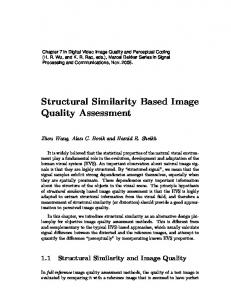
Fig. 1. Examples for FR quality index usage. (a) Compression algorithm assessment. (b) Restoration algorithm assessment. (Full resolution in color can be seen online in [34].)

Objective quality assessment, which is obtained by the visual quality matrix (VQM), is preferred over subjective quality assessment, which is obtained by the human observer. Subjective quality assessment through psychological experiments, representing human visual system (HVS) behavior, is the best known method for assessment of image quality. Nevertheless, HVS experiments are slow and expensive and give different results for the same set of inputs [2]. Objective quality assessment, on the other hand, is faster and cheaper and always gives the same score for the same set of inputs. Subjective quality assessment databases are available on the net [3]–[5] and can be compared to the objective score of the VQM. In this paper, we focus on a full-reference (FR) color image VQM. The degraded image is compared with a reference image , which is considered to have “perfect quality,” and difference mean opinion score (DMOS) [6] is created to represent the degradation score. A typical use for evaluation of such algorithms, with an FR VQM, is shown in Fig. 1. Evaluation of the quality performance of a compression algorithm [see Fig. 1(a)] can done by comparing the compressed image with the reference image. Evaluation of a restoration algorithm [see Fig. 1(b)] is done by implementing the restoration on a distorted version of the reference image, such as blur or desaturation, and comparing the restored image with the reference image. Every color pixel is composed from two perpendicular vectors, namely, luminance vector LV and chrominance vector CV, as shown in Fig. 2. Thus LV

CV

LV CV

(1)

,1 and CV LV. where LV HVS is much more sensitive to light intensity changes than it is to chrominance changes [7] and is also more sensitive to contrast than to mean shift [8]. The aforementioned facts are 1We chose to work in RGB color space, but one may also use our convention in YCbCr, Yuv, CIELAB, or any other tristimulus color space.

1057-7149/$26.00 © 2011 IEEE

KOLAMAN AND YADID-PECHT: QSSIM: NEW QUALITY INDEX FOR COLOR IMAGES

1527

Fig. 2. (a) Luminance vector LV and chrominance vector CV in . (b) Looking above on CV. (c) Color image LV CV . (d) Gray-scale image LV . (Full resolution in color can be seen online in [34].)

Fig. 3. Crosstalk effects in (a) old technologies (35 m) and (b) current sensors (18 m and 13 m) have color desaturation. (c) Future sensors will probably have a combined degradation of blur and desaturation. (Full resolution in color can be seen online in [34].)

suspected to be the reason why gray-scale VQMs (on the luminance vector) are still being extensively used and developed [9]–[13]. We will now review some of the existing state-of-the-art VQMs that are relevant references to our work. Singular value decomposition (SVD) is a method of transforming an image into its singular values, which is similar to the well-known eigenvalues from linear algebra. A gray-scale VQM based on SVD is described in [14]. This method divides each gray-scale image into 8 8 blocks and performs SVD transform to produce a singular value block. A new VQM based on the divisive normalization (DN) technique has been recently proposed in [15]. DN is based on a model that describes the early visual processing in the V1 cortex. Degraded and reference images are put into a pipeline transform made of wavelet transform , contrast sensitivity gain , and DN response to produce the difference image . The final score is computed using nonlinear summation. Structural SIMilarity (SSIM) [16] is a widely used VQM2 that has many versions, including a scaling version [17], a wavelet version [18], and a perceptual version [19]. Many researchers chose to combine the SSIM result with other measurements in order to expand it into color. Bianco et al. [20] combined an SSIM error map, which was preprocessed with a contrast sensitivity function (CSF), with CPSNR and a region-of-interest map using particle swarm optimization. Lee and Horiuchi [21] preprocessed each image with a CSF in the S-CIELAB color space and then performed SSIM on each color channel, which was averaged to give the final result. Shi et al. [22] combined SSIM with CPSNR using weighted addition, 60% SSIM, and 40% CPSNR ; they made a similar attempt in [23]. A comparison of some of the aforementioned VQMs is done in Section III. Gray-scale degradation mainly affects the size of the luminance vector, for example, blur and compression. Chrominance degradation mainly affects the size of the chrominance vector, for example, desaturation. Combined degradation affects both the luminance and chrominance vectors simultaneously, i.e.,

fect. CTK, in a CMOS image sensor, is a spatially variant blur kernel that currently degrades images by color desaturation [24], as shown in Fig. 3(b). It is expected that, in the future, smaller sensors will have a larger CTK kernel, which will introduce a combined degradation of blur and desaturation, as shown in Fig. 3(c). In this paper, we suggest building a combined VQM whose results are better correlated with human subjective tests and is able to work on images degraded by desaturation, blur, or a combination of both, as shown in Fig. 3. In addition, our new VQM has fair performance on all the other types of degradation in comparison with common state-of-the-art VQMs. This paper is organized as follows: Section II explains our work, Section III shows the testing we conducted to prove its efficiency, and Section IV gives the conclusions and future work to be done.

LV

LV

CV

CV

(2)

LV LV, and CV CV CV. where LV A need for a combined VQM arose when we wanted to measure a restoration algorithm for the color crosstalk (CTK) ef21873

cites according to Google scholar.

II. COMBINED DEGRADATION MEASUREMENT Here, we present the problem we tried to solve, which led us to our solution. The main aim of our research was to devise an automatic VQM that will evaluate the quality of an image degraded by the crosstalk effect. Because CTK is a combined degradation that combines blur with desaturation, we first tried using current state-of-the-art VQMs and did not get the result we wanted. In Section II-A, we show why it was difficult to use existing VQMs to measure a combined degradation. Section II-B presents the tool used in our solution, and Section II-C presents our new VQM. A. Measuring Combined Degradation With Current VQMs We choose to divide current state-of-the-art VQMs into three main categories. • Gray-scale VQMs—measuring the change in LV . Grayscale VQMs, such as mean-square error, peak signal-tonoise ratio (PSNR), SVD [14], and SSIM [16], [25], perform quality measurement on the size of the luminance vector and ignore the impact of color on image quality. These VQMs are able to predict the quality results for degradations on the luminance vector such as blur and compression noise but fail in predicting changes such as desaturation of color. • Chrominance VQMs—measuring the change in CV . Chrominance VQMs, such as colorfulness [26], perform measurement on the size of the chrominance vector (desaturation) and thus ignore the impact of luminance on image quality. Although they are able to predict the quality results for degradations on the chrominance vector such

1528

IEEE TRANSACTIONS ON IMAGE PROCESSING, VOL. 21, NO. 4, APRIL 2012

as desaturation, saturation, and color noise, they fail in predicting changes such as blur and compression noise on the luminance vector because they ignore the luminance vector impact. • Combined VQMs—measuring the change in . In our opinion, a combined VQM should measure three types of degradations, with good correlation to the human opinion score: 1) luminance-only degradations, such as blur; 2) chrominance-only degradations, such as desaturation; 3) combined luminance–chrominance degradations, such as blur combined with desaturation. To the best of our knowledge, we have not encountered a VQM that performs well on a combined degradation and gives an adequate match to human opinion. Some candidates for such a VQM were DN [15] and color SSIM (CSIM) [21]. We chose a SSIM VQM as a starting point for our work because it is well known for predicting human score luminance vector LV well,3 and adding color measurement to it would produce a better combined degradation measurement. Although this paper shows a color adaptation of a gray-scale VQM, i.e., SSIM, we believe that this framework can be used to adapt other gray-scale VQMs to color. One naive approach to expand existing VQMs into color is through linear combination of the separate results of each color space. We call this approach the dot-product approach and mark it as . For any VQM, this approach can be written as (3) where is any gray-scale VQM that we want to expand to color, is a VQM measurement on one of the color channels— , , or —where , , and are subparts of color vectors and . In our case, SSIM, which is an expansion of SSIM to color, i.e., CSIM. Thus CSIM

SSIM

SSIM

SSIM

(4)

. If we consider a single pixel in a color mark as image, a scalar cross correlation simplifies into

(5) The final result of (5) is a dot product between the two color vectors, which explains why we call the method presented in (3) the dot-product approach. papers we have encountered compare themselves to its results

and CV LV

into (b) and CV

with LV

and CV

with LV can be seen online in [34].)

with , (c) , and (d) and CV

. (Full resolution in color

Our main claim is that the dot-product approach is insufficient for measuring combined degradations in luminance and chrominance. To prove our claim, we consider a simple case of a synthetic image, as shown in Fig. 4(a),4 conLV CV , taining a single-color pixel and degrade it with a combined degradation as in (2) to produce LV CV . We wanted to with and test three degradation levels: , as shown in Fig. 4(b); with and , as shown in Fig. 4(c); and with and , as shown in Fig. 4(d). This case is very common when combined blur and desaturation are introduced because blur often brightens dark areas and desaturation makes , , and values become closer to their values. Calculating the scalar correlation between and its deusing (5), we get almost the same regraded versions sult for all three images, i.e., 0.353. As one can clearly notice, our eyes can sense the difference between the images, whereas the scalar cross correlation cannot, thus producing low correlation with our visual score. Our solution to this problem came from the origin of modern vector analysis, which will be reviewed in the following section. B. QIP

One of the main subparts of SSIM, which will be reviewed in Section II-C, is the scalar cross correlation, which we

3Most

Fig. 4. Simple test case, which represents combined degradations from (a) origwith LV inal pixel

Here, we will review the mathematical framework used to develop our new VQM—quaternion image processing (QIP). Using QIP, researchers expanded common image processing scalar tools, such as Fourier transform [27], correlation [28], and edge detection [29], into color vectors. This approach treats each color pixel as a single quaternion number and has relative low complexity in comparison with other vector approaches [29]. Quaternion space is the origin of modern vector analysis. It was first presented by Hamilton [30] 160 years ago. Hamilton is the inventor of the word “vector,” the dot product, and the cross product, which were derived from quaternion multiplication. Quaternion use was widespread until the beginning of the twentieth century (Maxwell’s equations were first formulated in quaternions). Later on, quaternions were replaced by modern vector analysis and have been long forgotten. In recent years, 4This example is in standard RGB color space but can be also illustrated in YCbCr, CIELAB, or any other tristimulus color space.

KOLAMAN AND YADID-PECHT: QSSIM: NEW QUALITY INDEX FOR COLOR IMAGES

scientists have cleared the dust off quaternions. With the use of quaternions, researchers found a more efficient way to calculate rotations in 3-D space. Modern applications for quaternions are found in computer graphics, physics, and aerospace flight dynamics A quaternion number has a real part and three imaginary parts and can be written as (6) , and , , and are its basic elements. where It is common to refer to in (6) as the quaternion scalar part, which is denoted by , and to as its vector part, , the quaternion which is denoted by . In the case where number is called a pure quaternion. In this paper, color pixels will be represented as a pure quaternion number . Addition and multiplication of quaternion numbers are associative as in familiar algebra. Multiplication is, however, not commutative and defined by the product rule of its basic elements, i.e., (7) and by the regular use of the distributive law. The quaternion conjugate is defined by (8)

1529

Fig. 5. Artificial image with luminance LV sinusoidally varying with from left to right in (a), marked as the continuous wave in (b). In this case, SSIM , marked as dashed line in components are as follows: average luminance (ac part), marked as the continuous line in (c); and contrast (b); LV component, marked as the dashed line in (d).

presented a holistic discrete Fourier transformation that treats a color pixel as a single number. He defined each color pixel as a pure quaternion number, i.e., (11) where , , and represent red, green, and blue values, respectively, and is the pixel location. From that, he defined a 3-D quaternion Fourier transform. This transform, which has many other versions, was later expanded by Said et al. to six dimensions in [32]. We chose quaternion algebra because it holds an implementation of vector cross correlation [28], as will be reviewed in Section II-C. C. Developing QSSIM

The quaternion modulus is defined by (9) Note that these definitions are consistent with regular complex numbers for any case where two of the three imaginary coefficients are zero, e.g., . Let be pure quaternion numbers, i.e., , and let and be their vector parts, respectively. Their multiplication is defined by the following standard quaternion multiplication:

(10) where is the standard dot product, and is the vector cross product. Vectorial scalar and cross multiplication were obtained by using the quaternion universal law given in (7). It is shown that any pure vector multiplication consists of two parts—its scalar part and its vector part . When measuring a multiplication relation between two vectors, as in the cross-correlation product, one should take into account both cross product and dot product as in (10). The reason for this is that when performing a dot product between two vectors, as in (3) and (5), we measure only part of the energy difference between the vectors. The field of QIP was first introduced by Sangwine [31] and has extensively expanded in the last decade. Sangwine

SSIM VQM has three parts, and to illustrate them, we have constructed an artificial example, as shown in Fig. 5(a), which has luminance LV sinusoidally varying with from left to right, marked as the continuous wave in Fig. 5(b). 1) —marked as the dashed line in Fig. 5(b). —marked as the continuous sine wave in 2) LV Fig. 5(c). 3) Contrast —marked as the dashed line in Fig. 5(d). Borrowed from electrical terminology, we chose to call the dc part and LV the ac part. Together, they form the scalar cross-correlation part— —which will be reviewed at the end of this section. Our color expansion named quaternion SSIM (QSSIM) has three parts, and to illustrate them, we have constructed an artificial example, which has luminance LV and chrominance CV sinusoidally varying with from left to right, as shown in Fig. 7(a) and its scatter plot in Fig. 7(e). Another artificial example is given in Fig. 8. 1) —marked as the center of the scatter plot in the examples in Fig. 8(a). 2) —shown as the scatter plot in Fig. 8(b). 3) Contrast —marked as the transparent sphere in Fig. 8(b). We now go over each subpart of SSIM and explain how we expanded them to QSSIM color VQM. The SSIM gray-scale average, which we define as the dc part, is calculated by averaging luminance vector LV over an image area, i.e., dc

LV

(12)

1530

IEEE TRANSACTIONS ON IMAGE PROCESSING, VOL. 21, NO. 4, APRIL 2012

Fig. 8. Subparts of QSSIM. (a) DC part of a color scatter plot. (b) AC part, ; contrast, marked as . marked as Fig. 6. Artificial example that has the same color object (ac part) from Fig. 7(a) with different background lights (dc part). (a) Red background. (b) Green background. (c) Blue background. Their matching scatter plots are shown in (d), (e), and (f), respectively. (Full resolution in color can be seen online in [34].)

Another example for a scatter plot with an indicator of the color dc part is shown in Fig. 8(a) and is placed at the center of mass for the scatter plot. Subtracting the background light (dc part) from the pixel will reveal the object, and we defined it as the ac part. The SSIM gray-scale ac part is defined as ac

Fig. 7. Artificial example with a constant background (dc part) with different degraded objects (ac part). (a) Full-color object. (b) Object with low color contrast. (c) Object with low luminance contrast. (d) Object with combined degradations. Their matching scatter plots can be seen in (e), (f), (g), and (h), respectively. (Full resolution in color can be seen online in [34].)

where LV is the luminance vector value of the image, and and describe the pixel location. A measuring example for the dc part of a synthetic image shown in Fig. 5(a) and its view presented as a sinus wave in Fig. 5(b) can be seen as the dashed line in Fig. 5(b). In this example, the dc part is a constant value that does not change over a certain area and will be always greater than zero, i.e., dc sup LV —where sup LV is the maximum possible value for luminance. In a gray-scale image, this is the background light. Our expansion to color vector average, which was defined in (12), was done by calculating the average of each color channel— , , and —separately and adding them to. Because vectors are gether— a subspace of quaternions, the above can be also defined in quaternions dc

(13)

LV

dc

LV

(14)

where dc is defined in (12). The object without the background light contains all the information needed for quality evaluation, and the ac part, which is marked as the continuous sinus wave in Fig. 5(d), is the object without its background light. Notice that the ac part can have positive or negative values. Our expansion to the color ac part is defined as ac

dc

(15)

where dc is defined in (13). The ac part of a color image is the color object without its background colored light. To illustrate , we have constructed an artificial example that has different objects (ac part) with the same background (dc part), as shown in Fig. 7(a). Another example for a scatter plot with an indicator of the color ac part is shown in Fig. 8(b), which is a scatter plot with its center of mass at the axis origin. SSIM gray-scale contrast is the average vector size of the ac part, i.e., ac

where ac is defined in (14). An image having high luminance contrast is considered to have better quality than a low-contrast image. A simplified 1-D version of (16) is shown in Fig. 5(d). Our expansion to color contrast was done using standard vector analysis by calculating (14) for each color channel—ac , ac , and ac —and then calculating ac

The average color is also called the centroid of the color scatter plot, which is now a 3-D vector in color space. In a color image, the dc part is the background light, which has brightness and color. To illustrate we have constructed an artificial example that has the same object from Fig. 7(a) with different background lights—red in Fig. 6(a), green in Fig. 6(b), and blue in Fig. 6(c).

(16)

,

where

ac ac ac ac is the vector size of ac ac ac ac . As in the case of average color, the above can be also defined in quaternions. Thus ac

(17)

KOLAMAN AND YADID-PECHT: QSSIM: NEW QUALITY INDEX FOR COLOR IMAGES

where ac is defined in (15). An artificial example of a scatter plot with an indicator of is shown in Fig. 8(b) as the transparent sphere inside the scatter plot of . Color contrast is now an indicator for three image quality degradation factors. 1) Luminance contrast—the amount of brightness span; a degradation example is shown in Fig. 7(c) and (g). 2) Color contrast (also known as colorfulness)—the amount of color in an image; a degradation example is shown in Fig. 7(b) and (f). 3) Combined contrast (color and luminance)—a degradation example is shown in Fig. 7(d) and (h). To illustrate the importance of the three contrast degradation types, we constructed an artificial example, with a degraded version of the ac part from Fig. 7(a), luminance contrast degradation in Fig. 7(c), color contrast degradations in Fig. 7(b), and combined degradation in Fig. 7(d). The aforementioned example shows why we think these degradations are important factors when measuring the quality of a color image, in which the quality of Fig. 7(d) seems lower than that of Fig. 7(c). This measurement capability is the main reason for using quaternion in our work. The main part in SSIM measuring the difference between two gray-scale images is the scalar cross correlation, which is defined by

ac

ac

(18)

where ac is defined in (14). Our expansion to color cross correlation, which is the main reason for using quaternions in our work, was defined in [28] as

ac

ac

(19)

where ref and deg are the reference and degraded images, respectively, is quaternion conjugate defined in (8), and ac , where is the dc part (also known as the centroid of the background light). If we take a single pixel, as in the example of Fig. 4, and take into account quaternion multiplication, from (10), (19) reduces to

1531

cross correlation, as in (5), measures only part of the vector correlation and thus lacks the ability to get good results for all types of degradations. Using a quaternion color correlation, given in (20), for the example given in Fig. 4, we get , , and , which shows a quality difference between the images. We believe that (19) is the key for the success of our new VQM because it measures both cross and dot products of two vectors and covers every type of change between the color vectors: 1) luminance degradation—as the example in Fig. 7(c); 2) chrominance degradation—as the example in Fig. 7(b); 3) combined degradation—as the example in Fig. 7(d). This leads to the QSSIM final version,5 which was composed to be the same as SSIM but with quaternion subparts,6 i.e., QSSIM

D. QSSIM Connection to SSIM SSIM is a special case of QSSIM because the latter measures direction and size and the former measures only size. Here, we will show how we can compress QSSIM into gray-scale SSIM and why, at the same time, SSIM cannot be expanded into QSSIM. We will now mathematically prove why a linear combination of SSIM, as suggested in Section II-A, cannot give QSSIM. Lemma 1: QSSIM

SSIM

SSIM

SSIM

(21)

is true for any values of , , and when measuring two different color images. Proof: Our proof is done on a single-color pixel but can be expanded into an entire color image. Because and (see explanation in Section II-C), we can divide (21) by the terms connected to these elements and get

Because we are dealing with a single-color pixel, we can simplify using (10) and get

The minus sign turns into a plus sign because we measure only the size of QSSIM. This leads us to (20) The aforementioned results show that a vector correlation is and composed of two parts, namely, scalar correlation cross correlation , which form color correlation . We can now explain why we failed in measuring a combined degradation, as presented in Fig. 4, by saying that using scalar

We know that

5Download 6We

it at http://www.ee.bgu.ac.il/kolaman/kolaman2011/.

chose to implement QSSIM in RGB color space, but it can also be used in YCbCr, CIELAB, or any other tristimulus color space

1532

IEEE TRANSACTIONS ON IMAGE PROCESSING, VOL. 21, NO. 4, APRIL 2012

TABLE II VQM COMPARISON USING THE RANK CORRELATION COEFFICIENT OUR DATABASE

Fig. 9. Subjective experiment samples of (a) reference image LV CV and its degraded versions with (b) CV CV CV

CV

CV, (d) CV, (f)

CV CV

CV, (c) CV, (e)

CV, and (g)

CV. (Full resolution in color can be seen online in [34].)

TABLE I VQM COMPARISON USING THE LINEAR CORRELATION COEFFICIENT FOR OUR DATABASE

three types of saturation levels, i.e., CV, CV, and CV. We created two sets of degraded images: the first three images, which are denoted by deg , deg , and deg , had a Gaussian blur with , and the second triplet, which are denoted by deg , deg , and deg , had . Each triplet has one full-color image with blur only and two desaturated images with CV CV, thus creating six degraded images for each source and image, i.e., LV

CV

BLR LV

which leads us to

Although one may find specific values of , , and for which (21) may not be true, these specific values will not be true for all the other cases. Adapting QSSIM into gray scale and getting the same results as SSIM can be done, because in this case, term in the color correlation goes to zero and leaves the scalar correlation. This can be done by scaling each color channel by and inputting the gray image into QSSIM. III. EXPERIMENTS AND TESTING Here, we describe the experiment on human subjects to test our hypothesis, in which we found an interesting connection between blur and desaturation. Testing and comparison between QSSIM and other VQMs was done on external databases, which shows the superiority of QSSIM over other state-of-the-art VQMs. A. Subjective Experiment of a Combined Blur/Desaturation Degradation Our main hypothesis is that a combined degradation of gray scale and color, such as desaturation with blur in the crosstalk effect, is an effect that can be measured well by our new VQM. To prove that, we had to build a database that included combined degradations of blur with desaturation. Doing our initial testing, we found that there must be a big enough difference between blurred images in order for the experiment to succeed. We chose two types of Gaussian blur degradations with and and combined them with

FOR

CV

BLR LV

CV

BLR LV

CV

BLR LV

CV

BLR LV

CV

BLR LV

CV

(22)

where BLR LV is a Gaussian blur with variance of . We expected to get a lower quality score as the image number increased, i.e.,

(23) where is the subjective quality score of a degraded image number . In our subjective experiment, we asked viewers, of both genders, with good eyesight and chromatic viewing capabilities (no color blindness) to give a quality score to a degraded image in comparison with its original image and produce a DMOS. Experiments were conducted under the same viewing conditions and a calibrated screen showing one of the original images, taken from [33], next to a degraded version. Each viewer was asked to view a set of 40 random image pairs, as shown in Fig. 9, and to give a quality evaluation of the degraded image using a slider with words describing quality. Slider position was then translated to a score between 1 for a very bad image and 100 for a perfect image. A total of 880 images were viewed by 20 viewers, of whom three viewers were rejected by an outlier rejection test. To build the DMOS, we averaged the -score for each viewer and normalized it to 1. Results from the experiment, which are available online [34], confirmed our hypothesis that blur and color desaturation have a combined impact on image quality. We found that blur has a

KOLAMAN AND YADID-PECHT: QSSIM: NEW QUALITY INDEX FOR COLOR IMAGES

TABLE III VQM COMPARISON USING THE LINEAR CORRELATION COEFFICIENT FOR THE IVC DATABASE

1533

TABLE VI VQM COMPARISON USING THE RANK CORRELATION COEFFICIENT FOR THE TID DATABASE

TABLE IV VQM COMPARISON USING THE RANK CORRELATION COEFFICIENT FOR THE IVC DATABASE

TABLE VII VQM COMPARISON USING THE LINEAR CORRELATION COEFFICIENT FOR THE LIVE DATABASE TABLE V VQM COMPARISON USING THE LINEAR CORRELATION COEFFICIENT FOR THE TID DATABASE

TABLE VIII VQM COMPARISON USING THE RANK CORRELATION COEFFICIENT FOR THE LIVE DATABASE

stronger impact on image quality and that desaturation creates subquality levels between two blurred images. This means that the quality score of degraded images deg , deg , deg , deg , deg , and deg shown in Fig. (b)–(g), respectively, matched (23).

The tables present the correlation between VQM and DMOS [6] results by calculating the Pearson’s linear correlation coefficient in Tables I, III, V, and VII and the Spearman’s rank correlation coefficient in Tables II, IV, VI, and VIII. Correlation was directly performed on the raw data from the VQMs. Comparison was made on four different databases of subjective HVS assessment. Tables III and IV belong to the IVC database [5]. Tables V and VI belong to the TID database [4]. Tables VII and VIII belong to the LIVE database [3].

B. Comparison Between QSSIM and Other VQMs

C. Analysis

We compared our new VQM, i.e., QSSIM, against common VQMs, such as color PSNR (CPSNR), SVD [14], and SSIM, and two color state-of-the-art VQMs, such as a DN matrix [15] and CSIM [22].7

Looking at Tables I and II, it is clear that our proposed QSSIM outperforms all the other VQMs in our subjective experiment. This confirms our hypothesis that QSSIM is able to measure combined degradation of blur and desaturation. Further detail can be extracted from the scatter plot and their fitting curves in Figs. 10–12.

7Other color VQM correlated poorly so that we chose not to present them in our comparison tables

1534

IEEE TRANSACTIONS ON IMAGE PROCESSING, VOL. 21, NO. 4, APRIL 2012

Fig. 10. Scatter plot with the linear fitting curves for our subjective experiment [34]. (a) Our proposed QSSIM. (b) SSIM [16]. (c) DN [15]. (d) CISM [21]. (e) SVD [14]. (f) CPSNR. (Full resolution in color can be seen online in [34].)

Fig. 11. Scatter plot with the linear fitting curves for LIVE subjective experiment [3]. (a) Our proposed QSSIM. (b) SSIM [16]. (c) DN [15]. (d) CISM [21]. (e) SVD [14]. (f) CPSNR. (Full resolution in color can be seen online in [34].)

QSSIM also performs well on other databases [3]–[5]. Looking at Tables III, IV, and VIII, it is clear that QSSIM is best correlated with HVS, outperforming other VQMs both in the overall performance and in most degradation types. In the linear case of Table VII, QSSIM is second best after DN. Looking at Tables V and VI, it is difficult to determine which VQM performs best. If we consider only the separate degradation types and disregard ambiguous results, where it is hard to determine which VQM is best, QSSIM clearly outperforms other VQMs in 5 and CISM in 4, and CPSNR is best in 3 out of 16 degradation types. IV. CONCLUSION AND FUTURE WORK In this paper, we have developed a new VQM for color images that combines quality measurement for degradations in luminance, chrominance, and a combination of both.

Our main claim is that such a VQM is necessary because some degradation in color images, such as CTK, affects both chrominance and luminance. We tested this hypothesis in a subjective experiment on human subjects and proved that HVS is sensitive to a combined degradation of blur and desaturation. Our experiment showed that blur has a stronger effect on image quality and that desaturation creates intermediate quality levels between blurred images. In order for this to occur, the difference between Gaussian blur types must be above a certain threshold. Correlation measurements on our database showed that QSSIM outperforms all other VQMs. We also showed how well QSSIM performs on three other external databases in comparison with several state-of-the-art VQMs. This paper provides a framework for extending existing grayscale VQMs into color using QIP. We believe that future work

KOLAMAN AND YADID-PECHT: QSSIM: NEW QUALITY INDEX FOR COLOR IMAGES

1535

Fig. 12. Scatter plot with the linear fitting curves for TID subjective experiment [4]. (a) Our proposed QSSIM. (b) SSIM [16]. (c) DN [15]. (d) CISM [21]. (e) SVD [14]. (f) CPSNR. (Full resolution in color can be seen online in [34].)

may include similar extensions of other gray-scale VQMs. Another future work will include a more extensive experiment with several types of Gaussian blur to determine the exact threshold difference that allows this quality model to stay consistent. ACKNOWLEDGMENT The authors would like to thank S. Sangwine for his generous help; D. Hasler and S. Susstrunk for making their saturation image database available for download and review; students L. Dotan and R. Harazi for their help; people who participated in their subjective experiment; the Associate Editor for his comments and review; and, finally, B. L. Coleman for his inspiration and love for quaternions. REFERENCES [1] Z. Wang and A. C. Bovik, “Modern image quality assessment,” Synth. Lectures Image, Video, Multimedia Process., vol. 2, no. 1, pp. 1–156, 2006. [2] A. M. Eskicioglu, “Quality measurement for monochrome compressed images in the past 25 years,” in Proc. ICASSP, 2000, pp. 1907–1910. [3] L. C. H. R. Sheikh, Z. Wang, and A. C. Bovik, “Live image quality assessment database release 2,” 2007. [Online]. Available: http://live. ece.utexas.edu/research/quality [4] N. Ponomarenko, V. Lukin, A. Zelensky, K. Egiazarian, M. Carli, and F. Battisti, “Tampere image database 2008,” 2008. [Online]. Available: http://www.ponomarenko.info/tid2008.htm [5] P. Le Callet and F. Autrusseau, “Subjective quality assessment IRCCYN/IVC database,” 2005. [Online]. Available: http://www.irccyn.ec-nantes.fr/ivcdb/ [6] H. Sheikh, M. Sabir, and A. Bovik, “A statistical evaluation of recent full reference image quality assessment algorithms,” IEEE Trans. Image Process., vol. 15, no. 11, pp. 3440–3451, Nov. 2006. [7] R. Hunt and E. Carter, The Reproduction of Colour. London, U.K.: Fountain Press, 1995. [8] M. Levine and J. Shefner, Fundamentals of Sensation and Perception. Boston, MA: Addison-Wesley, 1981. [9] D. Kim and R. Park, “New image quality metric using the Harris response,” IEEE Signal Process. Lett., vol. 16, no. 7, pp. 616–619, Jul. 2009. [10] H. Han, D. Kim, and R. Park, “Structural information-based image quality assessment using LU factorization,” IEEE Trans. Consumer Electron., vol. 55, no. 1, pp. 165–171, Feb. 2009.

[11] P. Ndjiki-Nya, M. Barrado, and T. Wiegand, “Efficient full-reference assessment of image and video quality,” in Proc. IEEE ICIP, 2007, vol. 2, pp. II-125–II-128. [12] G. Zhai, W. Zhang, X. Yang, and Y. Xu, “Image quality metric with an integrated bottom-up and top-down HVS approach,” Proc. Inst. Elect. Eng.—Vis., Image, Signal Process., vol. 153, no. 4, pp. 456–460, Aug. 2006. [13] E. Lam and K. Loo, “An image similarity measure using homogeneity regions and structure,” in Proc. SPIE, 2008, vol. 6808, pp. 680–811. [14] A. Shnayderman, A. Gusev, and A. Eskicioglu, “An SVD-based grayscale image quality measure for local and global assessment,” IEEE Trans. Image Process., vol. 15, no. 2, pp. 422–429, Feb. 2006. [15] V. Laparra, J. Munoz-Mari, and J. Malo, “Divisive normalization image quality metric revisited,” J. Opt. Soc. Amer. A, vol. 27, no. 4, pp. 852–864, Apr. 2010. [16] Z. Wang, A. C. Bovik, H. R. Sheikh, and E. P. Simoncelli, “Image quality assessment: From error visibility to structural similarity,” IEEE Trans. Image Process., vol. 13, no. 4, pp. 600–612, Apr. 2004. [17] Z. Wang, E. Simoncelli, and A. Bovik, “Multiscale structural similarity for image quality assessment,” in Proc. Conf. Rec. 37th Asilomar Conf. Signals, Syst. Comput., 2003, vol. 2, pp. 1398–1402. [18] Z. Wang and E. Simoncelli, “Translation insensitive image similarity in complex wavelet domain,” in Proc. IEEE Int. Conf. Acoust., Speech, Signal Process., 2005, vol. 2, pp. 573–576. [19] D. Rao and L. Reddy, “Image quality assessment based on perceptual structural similarity,” Pattern Recognit. Mach. Intell., vol. 4815, pp. 87–94, 2007. [20] S. Bianco, G. Ciocca, F. Marini, and R. Schettini, “Image quality assessment by preprocessing and full reference model combination,” in Proc. SPIE, 2009, vol. 7242, p. 724 20O. [21] J. Lee and T. Horiuchi, “Image quality assessment for color halftone images based on color structural similarity,” IEICE Trans. Fundam. Electron., Commun. Comput. Sci., vol. E91-A, no. 6, pp. 1392–1399, Jun. 2008. [22] Y. Shi, Y. Ding, R. Zhang, and J. Li, “An attempt to combine structure and color for assessing image quality,” in Proc. Int. Conf. Dig. Image Process., Mar. 2009, pp. 314–318. [23] Y. Z. R. Shi, Y. Ding, and J. Li, “Structure and hue similarity for color image quality assessment,” in Proc. Int. Conf. Electron. Comput. Technol., 2009, pp. 329–333. [24] K. Hirakawa, “Cross-talk explained,” in Proc. 15th IEEE ICIP, 2008, pp. 677–680. [25] P. Getreuer, “Color space converter,” 2006. [Online]. Available: http://www.mathworks.com/matlabcentral/fileexchange/7744-colorspace-convert [26] D. Hasler and S. Susstrunk, “Measuring colorfulness in natural images,” in Proc. SPIE, 2003, pp. 87–95.

1536

[27] T. Ell and S. Sangwine, “Hypercomplex Fourier transforms of color images,” IEEE Trans. Image Process., vol. 16, no. 1, pp. 22–35, Jan. 2007. [28] C. Moxey, S. Sangwine, and T. Ell, “Hypercomplex correlation techniques for vector images,” IEEE Trans. Signal Process., vol. 51, no. 7, pp. 1941–1953, Jul. 2003. [29] P. Denis, P. Carre, and C. Fernandez-Maloigne, “Spatial and spectral quaternionic approaches for colour images,” Comput. Vis. Image Understand., vol. 107, no. 1/2, pp. 74–87, Jul./Aug. 2007. [30] W. Hamilton, Lectures on Quaternions. Dublin, Ireland: Hodges and Smith, 1853. [31] S. Sangwine, “Fourier transforms of colour images using quaternion or hypercomplex, numbers,” Electron. Lett., vol. 32, no. 21, pp. 1979–1980, Oct. 1996. [32] S. Said, N. Le Bihan, and S. Sangwine, “Fast complexified quaternion Fourier transform,” IEEE Trans. Signal Process., vol. 56, no. 4, pp. 1522–1531, Apr. 2008. [33] A. Olmos and F. A. A. Kingdom, “McGill calibrated colour image database,” 2004. [Online]. Available: http://tabby.vision.mcgill.ca [34] A. Kolaman and O. Y. Pecht, “Combined blur de-saturation image database,” 2011. [Online]. Available: http://www.ee.bgu.ac.il/~kolaman/QSSIM Amir Kolaman received the B.Sc. degree in electrical engineering and the M.Sc. degree from Ben-Gurion University of the Negev, Beersheba, Israel, in 2005 and 2011, respectively, where he is currently pursuing the Ph.D. degree in the Laboratory of Autonomous Vehicles, Department of Electrical and Computer Engineering. He currently has four scientific papers, namely, two conference and two journal papers. His research interests include real-time color image processing, quaternion image processing, and application of the theory of relativity in color image processing.

IEEE TRANSACTIONS ON IMAGE PROCESSING, VOL. 21, NO. 4, APRIL 2012

Orly Yadid-Pecht (S’90–M’95–SM’01–F’07) received the B.Sc., M.Sc., and D.Sc. degrees from the Technion-Israel Institute of Technology, Haifa, Israel, in 1983, 1990, and 1995, respectively. She was a National Research Council (USA) research fellow from 1995 to 1997 in the areas of Advanced Image Sensors at the Jet Propulsion Laboratory (JPL)/California Institute of Technology (Caltech). In 1997 she joined Ben-Gurion University, as a member in the Electrical and Electro-Optical Engineering Departments. There she founded the VLSI Systems Center, specializing in CMOS Image Sensors. From 2003 to 2005, she was affiliated with the ATIPS Laboratory, University of Calgary, Canada, promoting the area of integrated sensors. Since September 2009, she is the iCORE Professor of Integrated Sensors, Intelligent Systems (ISIS), University of Calgary. Her main subjects of interest are integrated CMOS sensors, smart sensors, image processing hardware, micro and biomedical system implementations. She has published over 100 papers and patents and has led over a dozen research projects supported by government and industry. In addition, she has co-authored and co-edited the first book on CMOS Image Sensors CMOS Imaging: From Photo-transduction to Image Processing (Springer, 2004). She also serves as a director on the board of two companies. Dr. Yadid-Pecht has served on different IEEE Transactions editorial boards, was the general chair of the IEEE International Conference on Electronic Circuits and Systems (ICECS) and is a current member of the steering committee of this conference.