are simply conjunctions of connection and disconnection constraints of the form conn(Ji ... Instead of relying on a base station to coordinate the flow of ... can be extended without major modification to query-based model checking of LTL .... our approach is closely related to temporal logic query checking, introduced in [2],.
Query-Based Model Checking of Ad Hoc Network Protocols Anu Singh, C. R. Ramakrishnan, and Scott A. Smolka Department of Computer Science, Stony Brook University, Stony Brook, NY 11794-4400, USA E-mail: {anusingh,cram,sas}@cs.sunysb.edu
Abstract. A prominent source of complexity in the verification of ad hoc network (AHN) protocols is the fact that the number of network topologies grows exponentially with the square of the number of nodes. To combat this instance explosion problem, we present a query-based verification framework for AHN protocols that utilizes symbolic reachability analysis. Specifically we consider AHN nodes of the form P : I, where P is a process and I is an interface: a set of groups, where each group represents a multicast port. Two processes can communicate if their interfaces share a common group. To achieve a symbolic representation of network topologies, we treat process interfaces as variables and introduce a constraint language for representing topologies. Terms of the language are simply conjunctions of connection and disconnection constraints of the form conn(Ji , Jj ) and dconn(Ji , Jj ), where Ji and Jj are interface variables. Our symbolic reachability algorithm explores the symbolic state space of an AHN in breadth-first order, accumulating topology constraints as multicast-transmit and multicast-receive transitions are encountered. We demonstrate the practical utility of our framework by applying it to the problem of detecting unresolved collisions in the LMAC protocol for sensor networks.
1 Introduction An ad-hoc network (AHN) is a local area network (LAN) that is built spontaneously as wireless devices connect. Instead of relying on a base station to coordinate the flow of messages between nodes in the network, individual nodes forward packets to and from each other. Because of its ah-hoc nature, an n-node AHN can assume any one of the 2 possible O(2n ) topologies. A number of network protocols have been developed for AHNs, including routing, MAC-layer, and transport protocols. Due to the vast space of possible network topologies, the verification of AHN protocols is a computationally intensive if not intractable task. Consider, for example, the verification of the LMAC medium access control [13] protocol performed in [5]. (We also consider this protocol in Section 6.) The approach taken in [5] was to separately model check each of the possible network topologies (modulo isomorphism) for a fixed number of nodes in order to detect those that might lead to unresolved collisions. An unresolved collision occurs when neighboring nodes (connected by at most two links) without a common neighbor attempt to transmit within the same time slot; due to the lack of a common neighbor, the collision remains undetected. The problem with this approach is that as the number of nodes in the network grows, the number of possible topologies grows exponentially, posing an instance explosion problem for verification. To combat instance explosion, we present in this paper a new, constraint-based symbolic verification technique for ad-hoc network protocols. The basic idea behind our approach is as follows. As in [11], we represent AHNs as a collection of nodes of the form P : I, where P is a sequential process and I is an interface. An interface is a set
of groups, with each group corresponding to a clique in the network topology. Dually, a group is used as a local-broadcast (multi-cast) communication port. Two nodes in the network can communicate (are within each other’s transmission range) only if there respective interfaces have a non-null intersection (share a common group). To achieve a symbolic representation of an AHN, we treat process interfaces as variables and introduce a constraint language for representing topologies. Terms of the language are simply conjunctions of connection and disconnection constraints of the form conn(Ji , Jj ) and dconn(Ji , Jj ), respectively. Here, Ji and Jj are interface variables, and conn(Ji , Jj ) signifies that Ji and Jj are connected (Ji ∩ Jj 6= ∅), while dconn(Ji , Jj ) means that Ji and Jj are disconnected (Ji ∩ Jj = ∅). As such, each term of the language symbolically represents a set of possible topologies. Given this symbolic representation of AHNs, one can now ask model-checking queries of the form: under what evaluations (i.e. topologies) of the symbolic interface variables does the reachability property in question hold? Our symbolic reachability algorithm explores the symbolic state space of an AHN. A symbolic state is a pair of the form (s, γ), where s is a network state comprising both the locations of the component processes and valuations of their local variables, and γ is a term from our topology constraint language. A symbolic transition from (s, γ) to (s′ , γ ′ ) is constructed by adding constraints to γ to obtain γ ′ whenever a communication (local broadcast) occurs. Assuming the communication involves process Pi as the broadcaster, the following constraints will be added: those of the form conn(Ji , Jj ), where Pj is a process capable of performing a corresponding receive action and deemed to fall within the transmission range of Pi ; and those of the form dconn(Ji , Jk ), where Pk is also a process capable of performing a receive action and deemed not to fall within Pi ’s transmission range. We describe an efficient symbolic reachability algorithm to verify reachability properties of symbolic AHNs. We moreover show that our symbolic reachability algorithm can be extended without major modification to query-based model checking of LTL properties. To demonstrate the practical utility of our symbolic verification technique for AHN protocols, we applied it to the problem of detecting unresolved collisions in the above-described LMAC protocol [13]. Our results show that our symbolic approach to query-based model checking is highly effective: in the case of a 6-node network, our symbolic reachability algorithm explored only 2,082 symbolic topologies, compared to a possible 32,768 actual topologies. Moreover, all 2,082 symbolic topologies were considered in a single verification run. In contrast, for the same property, the authors of [5] considered no more than a 5-node network, using 61 separate verification runs, one for each unique (modulo isomorphism) concrete topology. Main Contributions. The rest of the paper is organized around our main technical results, which include the following: – Section 4 presents our modeling framework for AHNs, its concrete and symbolic semantics, and a correspondence result relating the two semantics. – Section 5 considers our query-based verification technique based on symbolic reachability analysis, and its extension to LTL properties. – Section 6 illustrates the practical utility of our technique by analyzing a formal model of the LMAC [13] protocol, a MAC layer protocol for sensor networks. Additionally, Section 2 discusses our concrete and symbolic representations for AHN network topologies, Section 3 describes related work, and Section 7 offers our concluding remarks and directions for future work. Due to space limitations, complete proofs are omitted.
1
2
1
4
2
3
4
3
(a) Topology with detected collision
(b) Topology with undetected collision
Fig. 1. Example topologies for collision and collision-detection in the LMAC protocol.
2 An Example of Topologies and Topology Constraints Below we illustrate the use of a constraint language for representing sets of network topologies. In the LMAC protocol of [13], which is used to allocate transmission slots in a sensor network MAC layer, collision, i.e. simultaneous transmission between two nodes with overlapping ranges, is detected by neighbors common to both nodes. Fig. 1(a) shows a network topology for which a collision between nodes 1 and 2 can be detected due to the presence of a common neighbor (node 4). Fig. 1(b) shows a topology for which a collision between 1 and 2 remains undetected since they do not share a neighbor. As described in Section 1, we consider AHN nodes of the form P : I, where P is a process and I is an interface. Further, an interface is a set of groups, with each group g representing a shared communication channel and dually corresponding to a clique in the network topology [11]. Figs. 2(a) and 2(b) provide a groupbased view and concrete representation based on process interfaces of the network topology of Fig. 1(a). A symbolic representation of the same topology is given in Fig. 2(c) using connection (conn) and disconnection (dconn) constraints over interface variables J1 –J4 , as mentioned in Sec. 1. The language in which symbolic topology constraints is expressed is formally described in Section 4. The symbolic representation permits us to compactly represent sets of topologies. For instance, consider the constraint conn(J1 , J2 ) ∧ conn(J1 , J4 ) ∧ conn(J2 , J3 ) ∧ conn(J3 , J4 ). This represents topologies that contain edges (1, 2), (1, 4), (2, 3) and (3, 4). The topologies in this set may or may not contain edges (1, 3) and/or (2, 4). Hence the above constraint represents four 4-node topologies, including the ones in Fig. 1. We use topology constraints when constructing a symbolic verification proof (by reachability or model checking) to consider a set of topologies simultaneously. These constraints may get refined as needed as we progress in the proof, corresponding to case splits among the set of topologies. The constraint representation and lazy case-splitting enable us to consider a large number of topologies simultaneously within a single verification run. 3 Related Work Our symbolic approach to query-based model checking of AHN protocols can be considered a form of constraint-based model checking. Traditionally this technique has been used for the verification of infinite-state systems [4, 10], data-independent systems [12], systems with non-linear arithmetic constraints [3], timed automata [7], and imperative infinite-state programs [6]. In these works, constraints were used to compactly represent sets of states of a system being verified. In contrast to these, our approach uses variables in the system specification (to represent interconnections) and
g1
1
2
AHN Π1≤i≤4 Pi : Ii I1 = {g1} I2 = {g1, g2} I3 = {g2} I4 = {g1, g2}
AHN Π1≤i≤4 Pi : Ji conn(J1 , J2 ) conn(J1 , J4 ) conn(J2 , J3 ) conn(J2 , J4 ) conn(J3 , J4 ) dconn(J1 , J3 )
(b) Concrete Representation of Interfaces
(c) Symbolic Representation of Interfaces
g2
4
(a) Group-Based View
3
Fig. 2. Concrete and symbolic views of network topology of Fig. 1(a).
finds their valuations (in this case, topologies) for which a property holds. In this sense, our approach is closely related to temporal logic query checking, introduced in [2], which addresses the following problem: given a Kripke structure and a temporal logic formula with a placeholder, determine all propositional formulas φ such that when φ is inserted in the placeholder, the resulting temporal logic formula is satisfied by the Kripke structure. Query checking has been extended in a number of ways, including query checking of a wide range of temporal logics using a new class of alternating automata [1]; the application of query checking to a variety of model exploration tasks, ranging from invariant computation to test case generation [9]; and its adaptation to solving temporal queries in which formulas may contain integer variables [15]. Recently, symbolic representation of the set topologies has been used in [8] to analyze ad hoc networks. The constraint language in that work can only express the presence of connections between nodes, and not the absence of connections, in contrast to our work. It should be noted that the undetected collision problem in the LMAC protocol (see Section 6) is due to absence of connections, and cannot be detected using the constraint language of [8]. As mentioned in Section 1, the correctness of the 4-node and 5-node LMAC protocol [13] has been previously established in [5] using the UPPAAL model checker for timed automata. By systematically considering all 11 topologies for the 4-node case and all 61 topologies for the 5-node case (modulo isomorphism), they report all network topologies for which collisions may remain undetected in the LMAC protocol. They also iteratively improve the protocol model so that the number of topologies for which the protocol may fail is reduced. In contrast, our query-based approach verifies a property related to unresolved collisions using a single symbolic reachability run, thereby allowing us to additionally consider the 6-node case. 4 Modeling Framework 4.1 Syntax We formally define the syntax and semantics of our framework. Systems in our framework are modeled as composition of nodes. Following the notion of separation of a node’s communication and computation behavior presented in the ω-calculus [11], we consider a node to consist of a process (computational behavior) and an interface (communication capability). We present the notations used in defining our framework, followed by formal definitions of the components of our framework, namely a process, an interface, a node, and a system. Let D be a non-empty domain with a set of operations F and relations R defined over it, and Var be a countable set of variables over domain D. For instance, D may be a set of finite integers, with F containing arithmetic operations, and R comprising
equality, dis-equality and relational operations over integers. Symbols x, y (possibly subscripted) range over elements of Var. An environment θ : X 7→ D, where X ⊆ Var is a mapping from variables in Var to values in domain D. Symbol Θ is used to denote the set of all environments over Var and D. We use E to denote the set of expressions, which are terms over elements of D ∪ Var ∪ F . Expressions are represented by symbol e (possibly subscripted). A primitive condition is a term with a symbol from R whose arguments are elements of E. A condition is a conjunction of primitive conditions. An assignment is of the form x := e, where x ∈ Var and e ∈ E. Following traditional programming language semantics, we use [[.]] to represent semantics for expressions, conditions and assignments. For an expression e, condition cond, and assignment asgn, [[e]] : Θ 7→ D, [[cond]] : Θ 7→ Bool, and [[asgn]] : Θ 7→ Θ are mappings from an environment to domain D, Bool = { true , false }, and an environment, respectively. Semantics of a single assignment can be extended to a set of simultaneous assignments in the standard way. The syntactic definition of a process is as follows. Definition 1 (Process) A process = hL, X, Σ, δ, l0, η0 i, is an extended finite state automaton over domain D, where: – L is a finite set of locations. – X ⊆ Var is a set of local variables for the process. – Σ is a finite set of action labels containing • b e, e ∈ E (broadcast action). • r (x), x ∈ X (receive action). – δ is a finite set of transitions. A transition is a tuple (l, α, l′ , hρ, ηi), where • l, l′ ∈ L are source and target locations, respectively. • α ∈ Σ is an action label. • ρ, a condition, is a transition guard. • η is a set of simultaneous assignments of the form x1 := e1 , . . . , xn := en , where the xi are pairwise distinct. – l0 ∈ L is the start location. – η0 is the set of initial assignments of the form x := c, ∀x ∈ X, and c ∈ D. In the above definition of a process, we require that a variable that is used in a receive transition should not be assigned in the same transition. An interface, represented by symbol I (possibly subscripted), is a finite set of names called group names. Group names are denoted by symbol g (possibly subscripted). We use I to denote the set of all interfaces. A node P : I denotes a process P with interface I. Henceforth we use n to denote the set {1, . . . , n}, and Pi , i ∈ n, to denote the process hLi , Xi , Σ, δi , l0,i , η0,i i over domain D. Definition 2 (Ad Hoc Network, AHN) For i ∈ n, Pi = hLi , Xi , Σ, δi , l0,i , η0,i i s.t. Xi ⊆ Var are pairwise disjoint, then Πi∈n Pi : Ii is an AHN. 4.2 Concrete Semantics We provide a labeled transition system (LTS) based semantics for AHNs. An LTS is a 4-tuple (S, Act, −→, s0 ), where S is a set of states, Act is a set of labels, −→ ⊆ S × Act × S is a ternary relation of labeled transitions, and s0 ∈ S is the initial state. α A labeled transition (s, α, t) ∈−→, is also represented as s −→ t.
Definition 3 (Semantics of an AHN) The semantics of an AHN Πi∈n Pi : Ii , denoted as [[Πi∈n Pi : Ii ]], is the LTS (S, Act, T, s0 ) such that: – S = L × Θ, where L = L1 × . . . × Ln , Θ is the set of all possible environments X 7→ D, X = X1 ⊎ · · · ⊎ Xn . – Act = {b v | v ∈ D}. bv
′
′
– −→ is such that (l, θ) −→ (l , θ′ ), where l = (l1 , . . . , ln ), l = (l1′ , . . . , ln′ ), θ′ = [[η]]θ, v = [[e]]θ if: • ∃i ∈ n: (li , b e, li′ , hρi , ηi i) ∈ δi , and • k = {k|(lk , r (xk ), lk′ , hρk , ηk i) ∈ δk , k ∈ n, k 6= i, Ii ∩ Ik 6= ∅}, such that : ∗ ∀j ∈ n \ (k ∪ {i}): lj′ = lj V ∗ ρ = ρi ∧ k∈k ρk , [[ρ]]θ is true S ∗ η = ηi ∪ k∈k ηk [v/xk ] ∪ {xk := v} S – s0 = (l0 , θ0 ), where l0 = hl0,1 , . . . , l0,n i, θ0 = [[ i∈n η0,i ]]θǫ , and θǫ is the empty environment. In the description of the transition relation (−→) in Definition 3, i denotes the index of a process capable of performing a broadcast (b e) action, and k denotes the set of indices of processes that are able to receive a value broadcast by process Pi . Note that processes not participating in the synchronization remain in the same location. For a transition to be enabled, the guards of synchronizing processes must be true. When a transition is taken, the value transmitted by the broadcaster is propagated to all receivers, and the assignments of the participating processes are performed. 4.3 Symbolic System Specification We define a symbolic semantics for AHNs in which process interfaces are treated as variables. For example, for a node P : I, I is treated as a variable in contrast to the concrete semantics, where I represents a set of group names. We use J to denote the set of interface variables and J (possibly subscripted) to denote elements of J. Topology Constraint Language. Constraints on process interface variables are given by the following grammar. Symbol Γ represents the constraint language and γ (possibly subscripted) represents elements of Γ . Γ ::= true | false | conn(J, J) | dconn(J, J) | Γ ∧ Γ A valuation ϑ : J → I maps an interface variable J to an interface I. A valuation ϑ is a model of a constraint γ, written as ϑ |= γ, defined as follows: ϑ |= true ϑ 6|= false ϑ |= conn(J1 , J2 ) if ϑ(J1 ) ∩ ϑ(J2 ) 6= ∅ ϑ |= dconn(J1 , J2 ) if ϑ(J1 ) ∩ ϑ(J2 ) = ∅ ϑ |= Γ1 ∧ Γ2 if ϑ |= Γ1 ∧ ϑ |= Γ2 A constraint of the form conn(J1 , J2 ) requires that nodes with interface variables J1 and J2 be connected, enabling them to communicate with each other. Constraint dconn(J1 , J2 ) requires nodes with interface variables J1 and J2 to be disconnected. A constraint γ is satisfiable, if there exists an interface valuation ϑ that assigns each interface variable in γ a value (set of group names) such that ϑ |= γ. Two constraints γ1 and γ2 are equivalent (≡) if for every valuation ϑ s.t. ϑ |= γ1 , it holds that ϑ |= γ2 , and vice-versa.
Proposition 1 Satisfiability of topology constraints is decidable. Proof Sketch: The following procedure determines the satisfiability of conjunction of primitive constraints over interface variables, and returns a satisfying assignment if there exists one. Consider a constraint γ over interface variables J1 , . . . , Jn . – Step 1: For every constraint of the form conn(Ji , Jj ), add a fresh name gij to Ji and Jj (so that Ji ∩ Jj 6= ∅). – Step 2: For every Ji that is not assigned a value in Step 1, initialize Ji to singleton set {gi }, such that gi has not been assigned to any interface variable in Step 1. – Step 3: For every constraint of the form dconn(Ji , Jj ), if Ji ∩ Jj = ∅, then constraint γ is satisfiable, otherwise γ is unsatisfiable. This procedure terminates and if γ is satisfiable, returns one satisfying assignment. ⊓ ⊔ For example, solution to the constraint conn(J1 , J2 ) ∧ conn(J1 , J4 ) ∧ conn(J2 , J3 ) ∧ conn(J3 , J4 ), is J1 = {g1,2 , g1,4 }, J2 = {g1,2 , g2,3 }, J3 = {g2,3 , g3,4 }, J4 = {g1,4 , g3,4 }. A symbolic AHN is an AHN for which topology is represented using interface variables. Definition 4 (Symbolic AHN) For i ∈ n, Pi = hLi , Xi , Σ, δi , l0,i , η0,i i s.t. Xi ⊆ Var are pairwise disjoint, then Πi∈n Pi : Ji is a symbolic AHN. Definition 5 (Semantics of a symbolic AHN) The semantics of a symbolic AHN Πi∈n Pi : Ji , denoted as [[Πi∈n Pi : Ji ]], is the symbolic LTS (S, Act, T, s0 ), such that: – S = L × Θ × Γ , where L = L1 × . . .× Ln , Θ is the set of all possible environments X 7→ D, X = X1 ⊎ · · · ⊎ Xn . – Act = {b v | v ∈ D}. bv
′
′
– ; is such that (l, θ, γ) ; (l , θ′ , γ ′ ), where l = (l1 , . . . , ln ), l = (l1′ , . . . , ln′ ), θ′ = [[η]]θ, v = [[e]]θ if: • ∃i ∈ n: (li , b e, li′ , hρi , ηi i) ∈ δi , and • k = {k|(lk , r (xk ), lk′ , hρk , ηk i) ∈ δk , k ∈ n, k 6= i}, ∃kc , kd : k = kc ⊎ kd such that: ∗ ∀j ∈ n \ (kc ∪ {i}): lj′ = lj V ∗ ρ = ρi ∧ k∈kc ρk , [[ρ]]θ is true S ∗ η = ηi ∪ k∈kc ηk [v/xk ] ∪ {xk := v} V V ∗ γ ′ = γ ∧ k∈kc conn(Ji , Jk ) ∧ k∈kd dconn(Ji , Jk ) is satisfiable S – s0 = (l0 , θ0 , true ), where l0 = hl0,1 , . . . , l0,n i, θ0 = [[ i∈n η0,i ]]θǫ , and θǫ is the empty environment. In the clause for transition relation (;) in Definition 5, i denotes the index of a process enabled to do a broadcast (b e) action, and k denotes the set of indices of processes that are enabled to perform a receive action. kc and kd form a partition of k such that kc is the set of indices of processes that synchronize with the Pi ; thus conn constraint is generated for processes in kc . Processes with indices in kd do not synchronize with broadcast action of Pi , and thus are not connected to Pi , and dconn constraint is generated for the transition. Note that, as in the concrete semantics, processes not involved in the synchronization remain in their locations. The guards and assignments are treated exactly as in the concrete semantics, considering only the synchronizing processes.
Theorem 2 (Correspondence) The symbolic semantics is sound and complete w.r.t. α the concrete semantics; i.e. (s, γ) ; (s′ , γ ′ ) in [[Πi∈n Pi : Ji ]] iff ∀ interface valuations α ϑ s.t. ϑ |= γ ′ , s −→ s′ in [[Πi∈n Pi : ϑ(Ji )]]. Proof Sketch: α – Soundness: Consider a symbolic transition (s, γ) ; (s′ , γ ′ ) in Πi∈n Pi : Ji . From ′ the semantics of the symbolic transitions, γ =⇒ γ. For all ϑ s.t. ϑ |= γ ′ (also α ϑ |= γ), there exists a concrete transition s −→ s′ in Πi∈n Pi : ϑ(Ji ). α – Completeness: Consider a concrete transition s −→ s′ in Πi∈n Pi : Ii . Let ϑ be an interface valuation, γ ′ be a constraint, and for i ∈ n, Ji be interface variables, α such that ϑ(Ji ) = Ii , and ϑ |= γ ′ . Then ∃γ : γ =⇒ γ ′ , and (s, γ) ; (s′ , γ ′ ) in Πi∈n Pi : Ji . ⊓ ⊔ 5 Constraint-Based Verification 5.1 Verification of Reachability Properties We first consider verification of symbolic AHNs for reachability properties, which is done by constructing and traversing the symbolic transition system. Definition 6 (Reachability) For an AHN AC = Πi∈n Pi : Ii , the set of states reachable from a state s in [[AC ]], denoted by ReachC (s, AC ), is the smallest set such that s ∈ ReachC (s, AC ) and for every s′ ∈ ReachC (s, AC ) and for every α ∈ Act if α s′ −→ s′′ ∈ [[AC ]] then s′′ ∈ ReachC (s, AC ) For a symbolic AHN AS = Πi∈n Pi : Ji , the set of states reachable from a symbolic state (s, γ) in the [[AS ]], denoted by ReachS ((s, γ), AS ), is the smallest set such that (s, γ) ∈ ReachS ((s, γ), AS ), and for every (s′ , γ ′ ) ∈ ReachS ((s, γ), AS ) and for α every α ∈ Act if (s′ , γ ′ ) ; (s′′ , γ ′′ ) then (s′′ , γ ′′ ) ∈ ReachS ((s, γ), AS ). Satisfaction of a Property. A property over a concrete AHN AC , denoted by φ is either a proposition, defined over the states of AC , or of the form EFp, where p is a proposition. We use s |= φ to denote satisfaction of property φ in state s. We say that s |= EFp if there is some state s′ reachable from s such that s′ |= p. The notion of satisfaction of a property is lifted to symbolic states, denoted as (s, γ) |= φ, if γ is satisfiable, and φ is true in s in every topology ϑ such that ϑ |= γ. The following proposition establishes that when verifying a reachability property for a symbolic AHN, it is sufficient to examine a subset of symbolic states. In particular, once (s, γ) is visited and (s, γ) |= φ, all states (s, γ ′ ) such that γ ′ =⇒ γ can be discarded from consideration. Proposition 3 For a given symbolic state (s0 , γ0 ), symbolic AHN AS , and property φ, if ∃(s, γ) ∈ ReachS ((s0 , γ0 ), AS ) s.t. (s, γ) |= φ, then ∀(s, γ ′ ) ∈ ReachS ((s0 , γ0 ), AS ) s.t. γ ′ =⇒ γ, (s, γ ′ ) |= φ. Algorithm SymReach (Fig. 3) uses Prop. 3 to prune the search space for proving reachability properties. For a given predicate p, a symbolic AHN and a start state (s0 , γ0 ) in the AHN, Algorithm SymReach returns the set of most general constraints CS such that for all γ ∈ CS (s0 , γ) |= EFp. The set of reachable states are stored in R and a working set W S is used to store unvisited states (Line 3) during a breadth-first traversal of the transition system. At the beginning of each iteration (Line 4) states in R−W S have been completely explored. Since each transition only adds to the topology constraints, we discard symbolic states whose topologies are already known to satisfy the reachability property (Line 8). Line 9 uses Prop. 3 to prune the search space. In Line 13, mg chooses the most general set of constraints from a given set of constraints.
1. 2. 3. 4. 5. 6. 7. 8. 9. 10. 11. 12. 13. 14.
Algorithm SymReach Input : predicate p ; symbolic AHN AS ; initial symbolic state (s0 , γ0 ) Output : CS the set of most general constraints in states that satisfy p and are reachable from initial state (s0 , γ0 ) R := {(s 0 , γ0 )} ff {γ0 } if (s0 , γ0 ) |= p CS := ∅ otherwise WS := {(s0 , γ0 )} // working set (FIFO queue) while (WS 6= ∅) let (s, γ) ∈ WS WS := WS \ (s, γ) α for each transition (s, γ) ; (s′ , γ ′ ) in [[AS ]] ′ if γ not subsumed by any constraint in CS if there exists no (s′ , γ ′′ ) ∈ R such that γ ′ =⇒ γ ′′ WS := WS ∪ {(s′ , γ ′ )} R := R ∪ {(s′ , γ ′ )} if (s′ , γ ′ ) |= p CS := mg(CS ∪ {γ ′ }) return CS
Fig. 3. Symbolic Reachability Algorithm
Algorithm SymReach returns the CS set upon termination. It is easily shown that for a finite-state AHN Algorithm SymReach terminates. The following theorem formally states the correctness of the algorithm: that the set of topology constraints computed by SymReach exactly covers the topology constraints in ReachS (Def. 6). Theorem 4 (Correctness) Let CS ′ = {γ | (s, γ) ∈ ReachS ((s0 , γ0 ), AS ), (s, γ) |= φ} be the set of all constraints that are part of the reachable symbolic states (s, γ) for which φ holds. Let CS be the set returned by Algorithm SymReach (Figure 3). Then ∀γ ′ ∈ CS ′ ∃γ ∈ CS : γ ′ =⇒ γ, and ∀γ ∈ CS ∃γ ′ ∈ CS ′ : γ ≡ γ ′ . The choice of breadth-first search (BFS) in Algorithm SymReach is important for the following two reasons. First, subsumption-based pruning of search space is more effective with BFS because general constraints are visited before more specific constraints. Secondly, the use of BFS makes it easy to show the tight bound on the total number of symbolic transitions, used in the complexity analysis. 5.2 Complexity Analysis for the SymReach Algorithm Consider a concrete AHN AC with n nodes. Let the total number of states in AC be |S|, and the total number of transitions in AC be |T | = O(|S|2 ). The time for reachability analysis from a given initial state in AC is bounded by the number of transitions and is 2 equal to |T | = O(|S|2 ). The total number of topologies for an n-node AHN is O(2n ). Therefore, the time complexity for exploring states reachable from a given state in all 2 2 n-node AHNs (all possible topologies) is O(2n ) × |T | = O(2n |S|2 ). Let AS = Πi∈n Pi : Ji be a symbolic AHN and AC the set of all concrete AHNs 2 ACj = Πi∈n Pi : Ii,j , where index j indicates one of the O(2n ) possible topologies for an n-node network. Recall that each state of AS is of the form (s, γ), where s is a location-environment pair, and γ is a topology constraint. Let |S| be the largest number
2
of states of any concrete AHN AC ∈ AC . Since the number of distinct γ’s is O(2n ), 2 the total number of symbolic states is bounded by O(2n |S|). The number of symbolic transitions is bounded by the total number of concrete transitions for all possible topologies. We can establish this bound by defining a 1-1 mapping between symbolic transitions from a symbolic state (s, γ) in AS to a transition from concrete state s in AC . Consider associating each state in R and WS with an index which is the length of the shortest path from the initial state to (s, γ). Now, let (s, γ) be the selected state with index i at some iteration of the algorithm. There is no state (s, γ ′ ) in R − WS (i.e. visited state) such that γ =⇒ γ ′ (due to the use of subsumption, line 9 of the algorithm). First consider the case when there is no other state (s, γ ′ ) in R with index i. It follows from Theorem 2 that for every concrete topology that satisfies γ, state s is reachable in i or fewer steps. In fact, there is a concrete topology ϑ |= γ for which the shortest path to reach s is of length i. The symbolic transition that placed (s, γ) in WS can then be mapped to the corresponding concrete transition in the topology given by ϑ. Now consider the case when there is another state (s, γ ′ ) in R with index i. If (s, γ) and (s, γ ′ ) can be reached using a single transition from a common state, say (s′′ , γ ′′ ), then the symbolic transition that placed (s, γ) in WS can then be mapped to the corresponding concrete transition in a topology that satisfies γ ∧ ¬γ ′ . Otherwise, (s, γ) and (s, γ ′ ) descend from two distinct states, both of which have the same index. We can then associate with the symbolic transition to (s, γ) the same concrete instance ϑ used to map the transition to its parent (and similarly with (s, γ ′ )). We now show that reachability computation over symbolic state space takes no additional time, in the asymptotic sense, than reachability over concrete state spaces. The main additional cost of symbolic reachability algorithm is constraint subsumption (line 9 of the algorithm). We can do this operation in amortized constant time, as follows. First, consider computing and storing the subsumption lattice for the constraints 2 a priori. The construction cost of this lattice is O(2n ) but is paid only once. We can associate a set, initially empty, with each constraint in the lattice. To determine whether (s, γ) should be added to R, we check if s is in the set associated with γ in the lattice. This check can be done in constant time. When (s, γ) is added to R, we add s to the sets 2 associated with constraints more specific than γ. This operation may take O(2n ) in the worst case, but note that an element s may be added to the set associated with γ at most 2 once, and hence maintaining this data structure incurs a total cost of O(2n |S|) over the 2 entire run of the algorithm. Hence symbolic reachability can be done in O(2n |S|2 ), the same complexity as that of the concrete algorithm. The space complexity is bounded by the size of the set of reachable states, R. The 2 number of elements of this set is 2n |S|. The size of each element is O(n2 ) due to the size of the topology constraint, but this factor gets down-played in the asymptotic case. 2 Hence the asymptotic space complexity for the symbolic algorithm is O(2n |S|). 5.3 Model Checking Symbolic AHNs. The symbolic transition system can be readily used for checking LTL properties of AHNs. We can use the standard procedure of constructing the product between a B¨uchi automaton (corresponding to the negation of a given LTL property) and the symbolic transition system and look for reachable accepting cycles in the product graph. Note that for every symbolic transition of the form (s, γ) ; (s′ , γ ′ ), it holds that γ ′ =⇒ γ. Hence it follows that if (s, γ) and (s, γ ′ ) are two states in a cycle, then γ ≡ γ ′ . Hence the con-
straint component of states in a cycle are all equivalent. Let (s1 , γ), (s2 , γ), . . . (sn , γ) be states in an accepting cycle such that (si , γ) ; (si+1 , γ) for 1 ≤ i < n, and (sn , γ) ; (s1 , γ). It follows from Theorem 2 that for every concrete topology ϑ such that ϑ |= γ, the states s1 , s2 , . . . , sn will be in an accepting cycle. Hence reachable good cycles in the symbolic case mean that there are reachable good cycles in the concrete case. This forms the basis for LTL model checking of symbolic AHNs. Model checking of other temporal logics such as CTL and CTL* can be performed over symbolic AHNs by using the standard algorithms over the symbolic transition system. From the complexity results for reachability checking, it follows that model checking for symbolic AHNs can be done in time and space comparable to the total time and space for model checking of concrete AHNs for all topologies. 6 Verification of the LMAC Protocol We built a prototype implementation of SymReach in the XSB logic programming system [14]. XSB adds the capability of memoizing inferences to a traditional Prologbased system, which simplifies the implementation of fixed point algorithms such as SymReach. Below we present the results of verifying the LMAC protocol [13], a medium access control protocol for wireless sensor networks, using this prototype. LMAC protocol for Wireless Sensor Networks The LMAC protocol aims to allocate each node in the sensor network a time slot during which the node can transmit without collisions. Note that for collision freedom, direct (one-hop) neighbors as well as two-hop neighbors must have pairwise different slots. The protocol works by nondeterministically assigning slots, and resolving any collisions that result from this assignment. We apply our query-based verification technique to this protocol to compute the set of topologies for which there are undetected and hence unresolved collisions. Protocol Description [13]. In schedule-based MAC protocols, time is divided into slots, which are grouped into fixed length frames. Every node is allocated one time slot in which it can carry out its transmission in a frame without causing collision or interference with other transmissions. Each node broadcasts a set of time slots occupied by its (one-hop) neighbors and itself. When a node receives a message from a neighbor it marks the respective time slot as occupied. The four phases of the LMAC protocol involved in allocating time slots to nodes are as follows. Initialization phase: a node listens on the wireless medium to detect other nodes. On listening from a neighboring node, the node synchronizes by learning the current slot number and transitions to the wait phase. Wait phase: a node waits for a random period of time and then continues with the discover phase. Discover phase: a node listens to its one-hop neighbors during one entire frame and records the time slots occupied by them and their neighbors. On gathering information regarding the occupied time slots, the node randomly chooses a time slot from the available ones (time slots that do not interfere in its one-hop and twohop neighborhood), and advances to the active phase. Active phase: a node transmits a message in its own time slot and listens during other time slots. When a neighboring node informs that there was a collision in the time slot of the node, the node transitions to the wait phase to discover a new time slot for itself. Collisions can occur when two or more one-hop or two-hop neighboring nodes choose the same time slot for transmission. Nodes causing a collision cannot detect the collision themselves, they need to be informed by their neighboring nodes about the collision. When a node detects a collision it transmits information about the collision in its time slot.
Passive LMAC Process : < L, X, Σ, δ, l0 , η0 > L = {init, init1, init2, listening0, recOne0, done0, choice0, choice, active, sent, listening, recOne, recT wo, collision detected} X = {Current, RecV ec, Counter, SlotN o, F irst, Second, Col, Collision} Σ = {r (msg(Sslot, Scollision, Sfirst)), r (eos), b msg(slot, collision, first)} l0 = init η0 = {Current := −1, RecV ec := ∅, Counter := 0, SlotN o := −1, F irst := ∅, Second := ∅, Col := −1, Collision := −1} Transitions (l, α, l′ , hρ, ηi) ∈ δ are given below: Init [r (msg(Sslot, , ))] init → init1 & Current′ := Sslot [r (eos)] init1 → listening0 & Current′ := (Current + 1)%f rame, Counter ′ := 0 [r (msg( , , ))] init1 → init2 [r (eos)] init2 → init Discover [r (msg( , , Sfirst))] listening0 → recOne0 & RecV ec′ := Sfirst, F irst′ := {Current} ∪ F irst [r (msg( , , ))] recOne0 → done0 & if Collision < 0 then Collision′ := Current, RecV ec′ := ∅ [r (eos)] done0 → choice0 & Current′ := (Current + 1)%f rame [r (eos)] recOne0 → choice0 & Current′ := (Current + 1)%f rame, Second′ := RecV ec ∪ Second, RecV ec′ := ∅ [r (eos)] listening0 → choice0 & Current′ := (Current + 1)%f rame [ ] choice0 & Counter < f rame − 1 → listening0 & Counter ′ := Counter + 1 [ ] choice0 & Counter >= f rame − 1 → choice & Second′ := F irst ∪ Second Choice [ ] choice & Second 6= AllSlots → active & SlotN o′ ∈ AllSlots \ Second, Second′ := ∅ [ ] choice & Second = AllSlots → listening0 & Counter ′ := −1, Collision′ := −1, F irst′ := ∅, Second′ := ∅ Active [bmsg(SlotN o, Collision, F irst)] active & Current=SlotN o → sent & Collision′:=−1 [ ] active & Current 6= SlotN o → listening Send [r (eos)] sent → active & Current′ := (Current + 1)%f rame Listen [r (msg( , Scollision, ))] listening → recOne & Col′ := Scollision, F irst′ := Current ∪ F irst [r (eos)] listening → active & Current′ := (Current + 1)%f rame [r (msg( , , ))] recOne → recT wo & if Collision′ < 0 then Collision′ := Current [r (eos)] recT wo → active & Current′ := (Current + 1)%f rame [r (eos)] recOne & Col 6= SlotN o → active & Current′ := (Current + 1)%f rame Collision Reported [r (eos)] recOne & Col = SlotN o → collision detected & F irst′ := ∅, RecV ec′ := ∅ Current′ := (Current + 1)%f rame, Counter ′ := 0, SlotN o′ := −1, Col′ := −1, Collision′ := −1 [ ] collision detected → listening0 Fig. 4. LMAC protocol model.
Modeling the LMAC protocol in our framework. Our encoding of the LMAC protocol in our framework follows the encoding used in [5]. We carry over the underlying assumption in the LMAC protocol, that the local clocks of nodes are synchronous. Since there is no support for modeling time in our prototype framework, we define a special timer node that informs other nodes about the end of a time slot by broadcasting an end of slot message. Nodes update their local information at the end of every time slot. An encoding of a process in an AHN model of LMAC is presented in Fig. 4. At the beginning, we assume that one distinguished node is “active” (i.e. in active location) and the rest are “passive” (i.e. in init location). Note that the figure gives the definition of a passive node; the definition of the active node is identical except for its initial state. The (symbolic) system specification for a 3-node network is shown below. A = timer : J1 | active node : J2 | passive node : J3 | passive node : J4 Transitions in Fig. 4 are specified in the form [label] l & ρ → l′ & η, where label is the label of the transition, l and l′ are the source and destination locations, ρ is the (optional) guard and η is the set of simultaneous assignments. We use the standard notation of primed variables to denote variables in the destination state. We use “epsilon” transitions (denoted by action label [ ] in the figure) to simplify the encoding. We can derive the epsilon-free description (as in the formal definition of AHNs, Defn. 1) using standard automata construction techniques. In our model of LMAC, locations init, init1 and init2 correspond to the initialization phase; locations listening0, recOne0, done0, choice0 and choice to the discover phase; and locations active, sent, listening, recOne, recTwo, and collision detected to the active phase. It should be noted that the wait phase of the protocol is not modeled, since its function is to only separate the initialization and discover phases by an arbitrary period of time. The length of a time frame i.e. number of slots (= 5 for 5-node network) is represented by frame, and AllSlots denotes the set of all time slots. The state variables of a node are: Current (the current slot number w.r.t. the beginning of a frame), RecVec (auxiliary set to record the slots occupied by one-hop and two-hop neighbors), Counter (used to count the number of slots seen by the node in a frame), SlotNo (slot number of the node), First (set of slots occupied by one-hop neighbors of the node), Second (set of slots occupied by two-hop neighbors of the node), Col (collision slot reported by another node), Collision (slot in which the node detects a collision). The parameters of messages (msg) exchanged between nodes are: Slot, Collision, and First variables of the sender node. Analysis of the LMAC protocol. The property “every collision is eventually detected” can be encoded in LTL as G(collision ⇒ F collision detected), where collision and collision detected are propositions that are true in states where collision and collision detection occur, respectively. Although LTL model checking of symbolic AHNs can be done as outlined in 5, our current prototype implementation supports only reachability checking. We hence checked a related property “there is a detected collision” (EF collision detected). Let CS be the set of all topology constraints computed using algorithm SymReach when checking for reachability of proposition collision detected. Let ϑ be a valuation such that ϑ 6|= γ for any γ ∈ CS. Note that in the LMAC protocol, there may be a collision between any two neighboring nodes. If γ does not represent a fully disconnected topology, then we can conclude that there is an undetected collision in γ. Hence, by checking for reachability of proposition collision detected, we can compute (a subset of) topologies which have undetected collision. Moreover, using this
Nodes 2 3 4 5 6
# Topologies Symbolic/Concrete 1/2 5/8 25/64 181/1024 2082/32768
# States
# Transitions
CPU Time
Memory (MB)
36 110 458 2204 29012
36 123 667 5223 110194
0.08 sec 0.24 sec 3.38 sec 69.51 sec 2 hr 51 min 46 sec
2.42 2.46 3.05 5.09 49.79
Table 1. Verification statistics for the LMAC protocol for detected collisions.
method is sound: if there is an undetected collision in some topology, we will find at least one representative. Verification Statistics and Results. We did symbolic reachability checking for 2- to 6-node networks. The performance results are shown in Table 1. The results were obtained on a machine with Intel Xeon 1.7GHz processor and 2Gb memory running Linux 2.6.18, and with XSB Prolog version 3.1. For 2- and 3-node cases there were no collisions. For 4-, 5- and 6-node cases, topologies containing one-hop neighboring (directly connected) node pairs that appeared in a ring in the topology and did not have a common direct neighbor were found to be in collision that remained undetected. The second column in the table gives two numbers ξs /ξc , where ξs is the number of symbolic topology constraints explored in a reachability run, i.e. the number of distinct γ such that (s, γ) ∈ R as per the algorithm in Fig. 3; and ξc is the total number of possible concrete topologies. Observe that for the 6-node case the number of symbolic topology constraints examined is smaller than the number of concrete topologies by a factor of more than 5. It should also be noted that the same property was verified for a 5-node network in [5] by using 61 separate verification runs, one for each unique (modulo isomorphism) concrete topology. In contrast, we verified a related property using a single symbolic reachability run. The third and fourth columns in Table 1 give the number of symbolic states and transitions explored, respectively; and the last two columns give the CPU time and total memory used. Observe that the performance of our prototype implementation is efficient enough to be used for topologies of reasonable size (e.g. 6 nodes). It should be noted that our technique and its implementation does not exploit the symmetry inherent in the problem by identifying isomorphic topologies. At a high level, symmetry reduction can be incorporated by using a check in line 9 of SymReach that recognizes constraints representing the same set of topologies modulo isomorphism. Doing so will enable the technique to scale to large network sizes. 7 Conclusions We presented an efficient query-based verification technique for ad hoc network protocols. Network topologies are represented symbolically using interface variables, and the model-checking process generates constraints on the topology under which a system specification satisfies a specified property. As such, a term in our constraint language compactly represents a set of concrete topologies that may lead to the satisfaction of the property in question. We demonstrated the practical utility of our approach by considering the verification of a medium access control protocol for sensor networks (LMAC) [13], identifying topologies under which collision may remain unresolved. The basic data structure for query-based verification is the symbolic transition system, where each state carries with it a topology constraint. If a symbolic state is reachable, then, for every topology satisfying its constraint, the corresponding concrete state
is reachable. This structure makes it possible to infer topologies under which reachability properties hold. As described in the paper, it is also possible to verify properties specified in temporal logics such as LTL over symbolic transition systems, inferring sets of topologies under which the properties hold. Extending our prototype implementation to handle verification with an expressive temporal logic is a topic of future work. There are several avenues for further improving the efficiency of the symbolic verification technique. Some of these are optimizations to common low-level operations, subsumption checks, while others are high-level state-space reductions, e.g. by exploiting symmetries in systems and topologies. In this work, the focus is on a verification technique and not on the modeling language. We considered ad hoc networks whose topology does not change with time. We deliberately considered only closed systems and chose a simple language that uses interfaces to separate node behavior from network topology as in the ω-calculus [11]. As part of our future work, we plan to extend this work to open systems specified in the ω-calculus, and consider compositional verification in that setting. Acknowledgements. We thank the anonymous reviewers for their valuable comments on an earlier version of this paper. This work was supported in part by NSF grants CNS0509230, CNS-0627447, CNS-0721665, and ONR grant N000140710928. References 1. G. Bruns and P. Godefroid. Temporal logic query checking. In LICS, pages 409–417, 2001. 2. W. Chan. Temporal-logic queries. In CAV, volume 1855, pages 450–463. Springer, 2000. 3. W. Chan, R. Anderson, P. Beame, and D. Notkin. Combining constraint solving and symbolic model checking for a class of a systems with non-linear constraints. In CAV, pages 316–327. Springer-Verlag, 1997. 4. G. Delzanno and A. Podelski. Model checking in CLP. In TACAS, pages 223–239. SpringerVerlag, 1999. 5. A. Fehnker, L. van Hoesel, and A. Mader. Modelling and verification of the LMAC protocol for wireless sensor networks. In IFM, pages 253–272, 2007. 6. C. Flanagan. Automatic software model checking via constraint logic. Sci. Comput. Program., 50(1-3):253–270, 2004. 7. L. Fribourg. Constraint logic programming applied to model checking. In In Proc. 9th Int. Workshop on Logic-based Program Synthesis and Transformation (LOPSTR’99), LNCS 1817, pages 30–41. Springer-Verlag, 1999. 8. F. Ghassemi, W. Fokkink, and A. Movaghar. Equational reasoning on ad hoc networks. In Proceedings of the Third International Conference on Fundamentals of Software Engineering (FSEN), 2009. 9. A. Gurfinkel, M. Chechik, and B. Devereux. Temporal logic query checking: A tool for model exploration. IEEE Trans. Software Eng., 29(10):898–914, 2003. 10. A. Podelski. Model checking as constraint solving. In Proceedings of the 7th International Symposium on Static Analysis (SAS), pages 22–37. Springer-Verlag, 2000. 11. A. Singh, C. R. Ramakrishnan, and S. A. Smolka. A process calculus for mobile ad hoc networks. In COORDINATION, pages 296–314, 2008. 12. B. S. Starosta and C. R. Ramakrishnan. Constraint-based model checking of dataindependent systems. In International Conference on Formal Engineering Methods (ICFEM), volume 2885 of Lecture Notes in Computer Science, pages 579–598. Springer, 2003. 13. L. van Hoesel and P. Havinga. A lightweight medium access protocol (LMAC) for wireless sensor networks: Reducing preamble transmissions and transceiver state switches. In 1st International Workshop on Networked Sensing Systems (INSS), pages 205–208, 2004. 14. XSB. The XSB logic programming system. http://xsb.sourceforge.net. 15. D. Zhang and R. Cleaveland. Efficient temporal-logic query checking for presburger systems. In ASE, pages 24–33. ACM, 2005.