Quotient method for controlling the acrobot S. S. Willson, Philippe Mullhaupt and Dominique Bonvin
Abstract— This paper describes a two-sweep control design method to stabilize the acrobot, an input-affine under-actuated system, at the upper equilibrium point. In the forward sweep, the system is successively reduced, one dimension at a time, until a two-dimensional system is obtained. At each step of the reduction process, a quotient is taken along one-dimensional integral manifolds of the input vector field. This decomposes the current manifold into classes of equivalence that constitute a quotient manifold of reduced dimension. The input to a given step becomes the representative of the previous-step equivalence class, and a new input vector field can be defined on the tangent of the quotient manifold. The representatives remain undefined throughout the forward sweep. During the backward sweep, the controller is designed recursively, starting with the twodimensional system. At each step of the recursion, a well-chosen representative of the equivalence class ahead of the current level of recursion is chosen, so as to guarantee stability of the current step. Therefore, this stabilizes the global system once the backward sweep is complete. Although stability can only be guaranteed locally around the upper equilibrium point, the domain of attraction can be enlarged to include the lowerequilibrium point, thereby allowing a swing-up implementation. As a result, the controller does not require switching, which is illustrated in simulation. The controller has four tuning parameters, which helps shape the closed-loop behavior.
I. INTRODUCTION Any system with fewer actuators than the number of configuration variables can be regarded as an under-actuated system. There are numerous control approaches for nonlinear systems ([1], [2], [3], [4]), but many of them cannot satisfactorily control under-actuated systems. The control of under-actuated nonlinear systems has been a challenge due to the complexity of the internal dynamics. In most cases, these systems are not feedback linearizable. In contrast, there is no difficulty with the control of linear under-actuated systems as long as they are controllable. The acrobot is an under-actuated system [5]. Control in the neighborhood of the upper equilibrium point can be achieved by linearizing the model around that point. Methods such as Linear Quadratic Regulator (LQR) are adequate to control the resulting linear model, but the domain of attraction is often small. As a consequence, it is not possible to achieve swing-up using the linear model only. The acrobot is not feedback linearizable [2]. Nevertheless, controllers have been designed based on pseudo–linearization [6] and approximate state-feedback linearization [7]. These methods try to achieve feedback linearization around a Laboratoire d’Automatique, technique Federale de sanne, Switzerland.
Station Lausanne,
9,
Ecole CH-1015
PolyLau-
[email protected] [email protected] [email protected]
trajectory. Furthermore, swing-up through partial feedback linearization has been proposed [8], which leaves marginally stable zero-dynamics and hence is incapable of stabilizing the system. Energy-based swing-up methods have also been suggested for the acrobot [8], [9]. With all these methods, switching to a linear controller is needed when the system reaches the upright equilibrium position. Control of the acrobot has also been attempted using the interconnection and damping assignment (IDA) method [10]. For a similar under-actuated problem, namely the inverted pendulum, a global strategy that can achieve both swing-up and balancing has been suggested in [11]. The method relies on (i) changing the reference for the pendulum in order to pump the required energy for the swing-up, and (ii) using a singular perturbation approach to stabilize the cart. The control strategy is developed only for a neighborhood of the upright position, and switching of the reference value is used to reach that region from any given initial condition. In the present work, a nonlinear controller will be designed to locally asymptotically stabilize the acrobot in the neighborhood of the upwards position. The domain of attraction will be tuned in order to include the lower equilibrium point so that the controller can achieve both swing-up and balancing. This is achieved by first constructing quotient manifolds to achieve approximate feedback form [12], which decomposes the system into subsystems of lower dimensions. Then, these small subsystems are stabilized one by one, thereby leading to the full controller. This method is based on feedback linearization [12], [13], but it differs from pseudolinearization [6] and approximate linearization [7], where the approximation is done at the transformation stage to alleviate the hindrance arising from the Frobenius condition [2]. In the proposed method, the approximation is done at the controller design stage to adequately handle the fact that the system does not satisfy the condition for feedback linearization. The next section introduces the acrobot model. Section III describes the forward and backward sweeps required for control design. Section IV presents simulation results for the controlled system, while concluding remarks are presented in the last section. II. ACROBOT DYNAMICS The model of the acrobot is derived in [8]. It has two configuration variables, q = [q1 , q2 ]T ∈ R2 , defined on the configuration space Q = S1 × S1 and the input torque u. The equation of motion can be written in the general form M (q)¨ q + h(q, q) ˙ + φ(q) = τ
where M (q) denotes the positive-definite inertia matrix, vector h(q, q) ˙ the centrifugal and Coriolis components, and φ(q) the gravitational component. The input vector τ = [0, u]T represents the generalized forces. Defining the state vector
The acrobot has four equilibrium points corresponding to u = 0, of which three are unstable, (0, 0, 0, 0), (0, π, 0, 0) and (π, π, 0, 0), and one is stable, (π, 0, 0, 0). The system is not feedback linearizable [2] since the distribution ∆ =span{g, [f, g], [f, [f, g]]} is not involutive [9]. III. CONTROLLER DESIGN The controller design consists of two stages or sweeps. The first stage builds a strict feedback form for the equations of motion by successively constructing diffeomorphisms. The second stage iteratively constructs a controller for this feedback form.
A. Forward Sweep
The forward sweep proceeds iteratively by producing a succession of systems, each one being one unit smaller in dimension than the previous one, until a smaller manageable system is obtained. These systems are then stabilized during the backward sweep. To illustrate a reduction step, assume that it is applied when the system is described by r states, that is, ' (T x = x1 x2 x3 . . . xr
Fig. 1.
The acrobot
and it can be written as
as x = (x1 , x2 , x3 , x4 )T = (q1 − π/2, q2 , q˙1 , q˙2 )T [9], and representing the equations of motion as x˙ = f (x) + g(x)u
(1)
gives the two smooth vector fields f (x) and g(x): x3 0 x4 0 f (x) = f3 , g(x) = g3 f4 g4 where f3
= +
f4
= − + −
g3
=
g4
=
γ(x2 ) =
1 {c2 c3 (x3 + x4 )2 sin x2 + c2 c4 sin x1 γ(x2 ) c23 x23 cos x2 sin x2 − c3 c5 g sin(x1 + x2 ) cos x2 } 1 {−(c2 + c3 cos x2 )(2x3 x4 + x24 )c3 sin x2 γ(x2 ) c2 c4 g sin x1 − c3 c4 g cos x2 sin x1 c1 c5 g sin(x1 + x2 ) + c3 c5 g cos x2 sin(x1 + x2 ) (c1 + c2 + 2c3 cos(x2 ))x23 c3 sin x2 } −(c2 + c3 cos x2 ) γ(x2 ) c1 + c2 + 2c3 cos x2 γ(x2 ) c1 c2 − c23 cos2 x2 .
The acrobot parameters are collected to give the following constants: 2 c1 = m1 lc1 + m2 l12 + I1
c4 = m1 lc1 + m2 l1
2 c2 = m1 lc2 + I2
c5 = m2 lc2
c3 = m2 l1 lc2
x˙ = f (x) + g(x)u. One constructs the diffeomorphism z = Φ(x) that cancels the first r − 1 components of the transformed vector field ∂Φ ∂x g(x). The diffeomorphism is constructed by finding r − 1 independent solutions φ1 (x), φ2 (x), . . ., φr−1 (x) of the following system (termed the Lagrange subsidiary system [14]): dx1 dx2 dxr = = ··· = g1 g2 gr To find all solutions, one selects an independent variable and rewrite the above system as a system of r − 1 first-order ordinary differential equations in r − 1 dependent variables. A set of r − 1 independent solutions, φ1 (x), φ2 (x), . . ., φr−1 (x), is complemented with the r-th component ψ(x) chosen such that ∂ψ g(x) $= 0. (2) ∂x The diffeomorphism then becomes: ' (T Φ(x) = φ1 (x) φ2 (x) · · · φr−1 (x) ψ(x) .
The consequence of these operations is that the onedimensional integral manifold of the vector field g(x) (a twisted one-dimensional curve in the x-space) becomes a straight line in the z-space aligned along the zr -direction. Each line parallel to the zr axis corresponds to an equivalence class in the space described by the states x1 , x2 , x3 , . . ., xr . Each class corresponds to a one-dimensional integral manifold of the input vector field g(x) and is described by the value of the r − 1 states z1 , z2 , . . ., zr−1 . The choice of a value of zr (defined as zr = ψ(x1 , x2 , x3 , . . . , xr ))
corresponds to the choice of a representative of the equivalence class associated with z1 , z2 , . . ., zr−1 . This is similar to the classical construction of the quotient group Z4 = {¯ 0, ¯1, ¯2, ¯3}, a finite group that is defined as the quotient of two infinite groups Z and 4Z i.e Z4 = Z/4Z. Each element of Z4 stands for an associated infinite set, e.g. ¯1 stands for {. . . , −7, −3, 1, 5, 9, . . .}. The key idea is that one can choose the representative of ¯ 1 as either 1, 5 or −7 without affecting the value of ¯ 1. For the case of our dynamic system, the quotient elements are represented by z1 , z2 , . . ., zr−1 , and a representative of the equivalence class associated with specific values of z1 , z2 , . . ., zr−1 is given by zr = ψ(x1 , x2 , x3 , . . . , xr ). As in the previous example, where the choice of 1, 5 or −7 does not affect ¯1, there are many ways of representing z1 , z2 , . . ., zr−1 using x1 , x2 , x3 , . . ., xr . This choice is left open throughout the forward sweep, which will provide useful degrees of freedom in the backward (controller-design) sweep. Remark 1: It is precisely the property that the choice of the representative does not affect the equivalence class which allows differing controller design until after the reduction stage is complete, i.e. without affecting the forward decomposition sweep. The procedure is systematic for feedback linearizable systems, for which the following two properties are guaranteed at each step of the forward reduction [12]: (i) Existence of a well-defined equivalence class, i.e. the choice of the representatives is independent of the forthcoming reduction steps. (ii) Existence of a suitable input vector field along the tangent of the quotient manifold. This vector field is determined by grouping terms in the transformed −1 (z), obtained after projection, so vector field ∂Φ ∂x f ◦Φ that it becomes the sum of a vector field independent of the equivalence class described by zr = ψ and a term that is the product of another vector field independant of zr times zr (i.e. the reduced system with state-space coordinates z1 , z2 , . . ., zr−1 is affine in the new input zr ). That is, it must be possible to express P r[r] =
∂Φ f ◦ Φ−1 (z)) ∂x fˆ(z1 , . . . , zr−1 ) + gˆ(z1 , . . . , zr−1 )zr (
Where P r[r] is defined as. Definition 1: The projection map of order r, P r[r] : r R → Rr−1 , is defined as P r[r] ((a1 , a2 , ..., ar−1 , ar )T ) = (a1 , a2 , ..., ar−1 )T . Let us compute the successive steps for the non-feedbacklinearizable acrobot and see to what extent the Frobenius integrability condition [12] hinders meeting Properties (i) and (ii) described above. We will also explain how this hindrance can be overcome. The algorithm is initiated with g(x) = (0, 0, g3 , g4 )T , i.e. with r = 4. Property (i) holds since the system (1) has an equivalence class defined by a onedimensional manifold whose tangent is g(x). To determine
the quotient manifold, the first step is to solve ∂φi g(x) = 0 ∀ i = 1, 2, 3, ∂x for example, using the Lagrange subsidiary equations
(3)
dx2 dx3 dx4 dx1 = = = . 0 0 g3 g4 This set of equations becomes a system of ordinary differential equations with, for example, the independent variable chosen as x4 , while x1 , x2 , and x3 represent the dependent variables. Because the first two denominators are zero, the system dx1 dx2 g4 dx3
= 0 = 0 = g3 dx4
can be solved one equation at a time, which yields solutions that satisfies (3). Furthermore, let us choose ψ(x) = x3 to satisfy (2). It follows from φ1 (x) x1 φ2 (x) x2 = (c1 + c2 + 2c3 cos x2 )x3 (4) φ (x) Φ(x) = 3 +(c2 + c3 cos x2 )x4 ψ(x) x3
that
rank
)
∂Φ(x) ∂x
*
= 4.
Now define z ! Φ(x) with z ∈ R4 so that (4) is a diffeomorphism with the inverse x = Φ−1 (z): z = z˙ = =
Φ(x) ∂Φ(x) ∂Φ(x) f (x)|x=Φ−1 (z) + g(x)|x=Φ−1 (z) u ∂x ∂x fz (z) + gz (z)u (5)
By construction of Φ(x), the first 3 components of gz (z) are zero, i.e. gz (z) = (0, 0, 0, ∗)T . Application of the projection map of order 4 to System (5), ˙ = P r[4] (fz (z) + gz (z)u), P r[4] (z) removes the 4th component of the state. Since P r[4] (gz (z)) = (0, 0, 0), we obtain the following system: z˙1 fz1 (z) z˙2 = fz2 (z) z˙3 fz3 (z) z4 −z3 +(c1 +c2 +2c3 cos z2 )z4 (6) = c2 +c3 cos z2 g(c4 sin z1 + c5 sin(z1 + z2 )) Here, zˆ ! (z1 , z2 , z3 )T ∈ R3 defines a point on the quotient manifold, that is, a specific equivalence class. A representative of the equivalence class is given by a particular value of the z4 coordinate. Hence, Property (i) is fulfilled.
Note that, by construction, the input vector field gz (z) only affects the time derivative of the representative coordinate z4 : z˙4 = fz4 (z) + gz4 (z)u
(7)
with fz4 (z) and gz4 (z) the 4th elements of fz (z) and gz (z) defined in (5). The image of the input vector field gz (z) on the tangent of the quotient manifold is zero. Note that (6) is affine in z4 even though f3 and f4 contain quadratic terms in x3 and x4 . That is, the diffeomorphism has eliminated the quadratic terms in fz (z), which was possible because the distribution ∆ = span{g, [f, g]} is involutive ( [12] [13]). Hence, Property (ii) is also fulfilled, and the quotient dynamics read: zˆ˙ = fˆz (ˆ z) + gˆz (ˆ z)z4 (8) with fˆz (ˆz)
gˆz (ˆz)
=
0 −z3 c2 +c3 cos z2
g(c4 sin z1 + c5 sin(z1 + z2 )) 1 2 +2c3 cos z2 ) = (c1 +c , c2 +c3 cos z2 0
and the coordinate z4 acting as the new input. To obtain the next quotient manifold, the Lagrange subsidiary system for gˆz (ˆ z) is considered: (c2 + c3 cos z2 )dz2 dz3 dz1 = = , 1 (c1 + c2 + 2c3 cos z2 ) 0 which yields the following set of differential equations to be solved: (c2 + c3 cos z2 )dz2 dz1 = (c1 + c2 + 2c3 cos z2 ) dz3 = 0. Solving these equations gives the first two functions of the next diffeomorphism, while the third function is chosen to satisfy (2): z1 − ζ(z2 ) z3 Φz (ˆz) = z2 where ζ(z2 ) =
+
(c2 + c3 cos z2 ) dz2 . (c1 + c2 + 2c3 cos z2 )
Let y = (y1 , y2 , y3 )T ! Φz (ˆ z), which gives: y1 + ζ(y3 ) . y3 zˆ = Φ−1 z (y) = y2 Applying the projection map gives y2 y˙ 1 = c1 + c2 + 2c3 cos y3 y˙ 2 = g(c4 sin(y1 + ζ(y3 )) +
c5 sin(y1 + ζ(y3 ) + y3 )),
ˆ = (y1 , y2 )T defines a point on the quotient manifold where y and y3 is a representative of the equivalence class. Property (i) holds since the system (8) has an equivalence class defined by a one-dimensional manifold whose tangent is gˆz (ˆz). Since equations (9) and (10) are not affine in y3 , Property (ii) is not satisfied. The dynamics inside the equivalence classes determine the rate at which the representative y3 changes. This rate depends on the coordinate y2 and y3 of the point on the quotient manifold: (c1 + c2 + 2c3 cos y3 ) y2 + z4 .(11) y˙ 3 = c2 + c3 cos y3 (c2 + c3 cos y3 ) Note that equations (9) and (10) are similar to those for a free fall under gravity, where the gravitational acceleration term is manipulated using the input y3 . The variables y1 and y2 are expressed using the original state space as y1
=
q1 − ζ(q2 )
y2
=
(c1 + c2 + 2c3 cos(q2 ))q˙1 + (c2 + c3 cos(q2 ))q˙2
Equations (9), (10), (11) and (7) represent an alternate feedback form of the acrobot equations. This transformation is similar to that suggested in [15] to derive a cascade normal form for the acrobot. In fact, (9) and (10) are the same equations, while (11) and (7) are different. Note that it is possible to arrive at the cascade normal form using the quotient method by appropriately using the degree of freedom at each step. However, the quotient method is more general and does not exploit any specific property of under-actuated mechanical systems as opposed to the method suggested in [15]. B. Backward Sweep This section develops a controller for the acrobot based on the feedback form obtained in the preceding section. For this purpose, the following lemma will be used recursively. Lemma 1: Consider the system z˙ y˙
= =
f (z, y) p(y)
and assume that y˙ = p(y) has an asymptotically stable equilibrium point at y = 0. If z˙ = f (z, 0) has an asymptotically stable equilibrium at z = 0, then System (12) has an asymptotically stable equilibrium at (z, y) = (0, 0). This result is provided in Appendix B.2 of [2]. The following corollary of this lemma will help design the controller. Corollary 1: Consider the system x˙ = fx (x, ξ) ξ˙ = fξ (x, ξ) + g(x, ξ)u
(9) (10)
(12)
(13) (14)
where x ∈ Rn−1 , ξ ∈ R, u ∈ R, fx : Rn → Rn−1 , fξ : Rn → R and g : Rn → R with the equilibrium point (x, ξ) = (0, 0), and g(x, ξ) $= 0 in the domain of operation. If there exists ξd (x), with ξd (0) = 0, that asymptotically stabilizes System (13), then u
=
∂ξd ∂x fx (x, ξ)
− fξ (x, ξ) + k(ξd (x) − ξ) , (15) g(x, ξ)
where k is any arbitrary positive constant, locally asymptotically stabilizes both (13) and (14). Proof: Let the error variable be e
= ξd (x) − ξ.
(16)
TABLE I PARAMETERS USED FOR SIMULATION l1 1m
l2 2m
m1 1kg
m2 2kg
I1 0.083kgm2
I2 0.667kgm2
Substituting (16) and (15) into (13) and (14) gives the new set of equations x˙
= fx (x, ξd (x) − e)
(17)
e˙
= −ke
(18)
Using Lemma 1, it can be shown that the above system is locally asymptotically stable since • e = 0 is an asymptotically stable equilibrium of (18), ˙ = fx (x, ξd (x)) is also • for e = 0, by assumption, x asymptocically stable at x = 0. Hence, the system described by (17) and (18) is locally asymptotically stable at (x, e) = (0, 0), which implies that the system is locally asymptotically stable at (x, ξ) = (0, 0). This proof suggests that locally stabilizing the e-dynamics achieves local stability of (13) and (14). This method is similar to cascade design [16], and global stability can be achieved under certain conditions as outlined in [16]. This approach is used recursively to obtain the controller for the full system. For System (9), it is desired to have a function y2d (y1 ) that, when subsituted for y2 , gives asymptotically stable y1 dynamics. The presence of y3 in the denominator of (9) is immaterial. The denominator is always positive since it represents the first component of the mass matrix M (q). Hence, y2d ! −k1 y1 , with k1 any positive gain, stabilizes y1 . The error dynamics read: e1
= =
y2 − y2d y2 + k1 y1 .
Differentiating the error dynamics with respect to time gives e˙ 1
=
y˙ 2 + k1 y˙ 1 ,
To obtain the function y3d (y1 , y2 ) that makes e1 → 0 as t → ∞, the dynamics given by (18) are used. In particular, e˙ 1 = −k2 e1 , and substituting from (9) and (10) gives: y2 −k2 e1 = c1 + c2 + 2c3 cos y3d +k1 [g(c4 sin(y1 + ζ(y3d )) +c5 sin(y1 + ζ(y3d ) + y3d ))], where k2 is any positive gain. Since it is not possible to obtain a closed-form solution for y3d , the equation is linearized around the equilibrium point, which gives the following solution for y3d : y3d
= +
(c1 + c2 + 2c3 )(c4 g + c5 g + k1 k2 ) y1 (c2 c4 + c3 (c4 − c5 ) − c1 c5 )g k1 + (c1 + c2 + 2c3 )k2 y2 (c2 c4 + c3 (c4 − c5 ) − c1 c5 )g
Designing y3d through linearization considerably reduces the domain of attraction. Nevertheless, only a locally stabilizing controller is required, which is obtained through this linearization. Next, consider the system described by (9), (10) and (11). A stabilizing y3d is known for (9) and (10), which allows constructing e2 = y3 − y3d and by assigning e˙ 2 = −k3 e2 (using (15) ), gives z4d that will stabilize the system. Similarly, when the full system described by (9), (10), (11) and (7) is considered, the knowledge of z4d allows constructing e3 = z4 − z4d and assigning e˙ 3 = −k4 e3 gives u that locally asymptotically stabilizes the system around (0, 0, 0, 0). The stable open-loop equilibrium point (π, 0, 0, 0) is no longer an equilibrium point of the closedloop system. Due to the presence of tan(x2 /2) in ζ(x2 ), the other two equilibrium points become singularity points, where ζ(x2 ) is no longer defined. This represents an obstacle for obtaining a large domain of attraction. However, this does not prevent implementing the swing-up, as shown through simulation in the next section. IV. NUMERICAL SIMULATION This section illustrates the controller design of the previous section. The parameters used in this simulation are given in Table I [9]. To determine the controller gains k1 , k2 , k3 , k4 , the closedloop system is linearized around (0, 0, 0, 0) and the gains determined so that all four eigenvalues are at −1, which results in k1 = 10, k2 = 1, k3 = 1, k4 = 1. Three sets of simulations are presented. The first one corresponds to the swing-up of the acrobot, i.e. with initial conditions corresponding to the lower equilibrium point (π, 0, 0, 0). The second simulation illustrates the swing-up from the perturbed lower equilibrium point (π, 0.1, −0.2, −0.3). The last simulation shows stabilization from the arbitrary initial condition (π/2, π/2, 1, 1). The state trajectories are represented in Fig. 2 and Fig. 3, from which the following observations can be made: 1) The trajectories first come together before converging to the origin. Indeed, since the controller is designed to stabilize the error dynamics, as soon as the errors come close to zero, the behavior is the same irrespective of the initial conditions. 2) The angular velocities x3 and x4 reach very large values in all three cases, which calls for smaller controller gains. 3) Since sharp changes in angular velocities require large torques, the controller gains require tuning before practical implementation.
Swing up Swing-up: perturbed General initial condition
x1 3 2 1
2
4
6
8
10
12
14
time t
1 2
(a) x1
Swing up Swing-up: perturbed General initial condition
x3 80 60 40 20 2
4
6
8
10
12
14
time t
20 40 60
(b) x3 = x˙ 1 Fig. 2. Position and velocity of the first link for different initial conditions
x2
Swing up Swing-up: perturbed General initial condition
12 10 8
particular set of gains, finding an analytical proof requires further work. The method is straightforward to implement for feedback linearizable systems. For non-feedback-linearizable systems, however, direct implementation is not possible since the design requires the distribution ∆ = span{g, [f, g]} to be involutive at every step of the reduction process. Hence, each non-feedback-linearizable system needs to be investigated individually. This was undertaken here for the acrobot, for which a local linerization of the two-dimensional quotient dynamics led to a nonlinear stabilizing controller. The pendubot and the inverted pendulum are more difficult to deal with since the distribution ∆ = span{g, [f, g]} is not involutive at the first step already. On the other hand, the systematic nature of the method makes it likely to be turned into a numerical technique which can be used for a larger class of systems. Finally, the problem of input saturation has not been addressed in this paper. Further work could consider adapting the quotient method to handle the input saturation problem. VI. ACKNOWLEDGMENTS Supported by the Swiss National Science foundation grant FN 200021-11753/1 R EFERENCES
6 4 2
2
4
6
8
10
12
14
time t
(a) x2
Swing up Swing-up: perturbed General initial condition
x4 200
100
2
4
6
8
10
12
14
time t
100
200
(b) x4 = x˙ 2 Fig. 3. Position and velocity of the second link for different initial conditions
V. CONCLUSIONS AND FUTURE WORK A nonlinear controller design capable of swinging-up and balancing the acrobot at its upright position has been presented. Although the controller is local, the domain of attraction has been enlarged to achieve swing-up from its lower equilibrium point. Hence, a single controller achieves both swing-up and balancing as opposed to most previous attempts, where two different control strategies are required (one for swing-up and another for balancing). Locally stabilizing (balancing) behaviour of the controller is validated using Lyapunov’s first method and is guaranteed for all set of positive controller gains. The domain of attraction can be enlarged by appropriate choice of these gains. Although the swing-up capability has been validated in simulation for a
[1] H. K. Khalil. Nonlinear Systems. Prentice-Hall, Englewood Cliffs, N.J., 3rd edition, 2002. [2] A. Isidori. Nonlinear Control Systems. Springer Verlag, Berlin, Heidelberg, New York, second edition, 1989. [3] H. Nijmeijer and A. van der Schaft. Nonlinear Dynamical Control Systems. Springer Verlag, New York, 1990. [4] M. Krstic, P. V. Kokotovic, and I. Kanellakopoulos. Nonlinear and Adaptive Control Design. John Wiley & Sons, Inc., New York, NY, USA, 1995. [5] R. M. Murray and J. Hauser. Nonlinear controllers for non-integrable systems: the acrobot example. Proceedings of American Control Conference, pages 669–671, 1990. [6] S. A Bortoff and M. W. Spong. Pseudolinearization of the acrobot using spline functions. Proceedings of IEEE Conference on Decision and Control, 1(8):593–598, 1992. [7] S. A Bortoff. Approximate state-feedback linearization using spline. Automatica, 33(8):1449–1458, 1997. [8] M. W. Spong. The swing up control problem for the acrobot. Control System Magazine, IEEE, 15(1):49–55, 1995. [9] A Mahindrakar and R. Banavar. The swing up of acrobot based on a simple pendulum strategy. International Journal of Control, 78(6):424–429, 2005. [10] A Mahindrakar, A. Astolfi, R. Ortega, and G. Viola. Further constructive results on interconnection and damping assignment control of mechanical systems: The acrobot example. American Control Conference, pages 5584–5589, 2006. [11] B. Srinivasan, P. Huguenin, and D. Bonvin. Global stabilization of an inverted pendulum - Control strategy and experimental validation. Automatica, 45:265–269, 2009. [12] Ph. Mullhaupt. Quotient submanifolds for static feedback linearization. Systems & Control Letters, 55:549–557, 2006. [13] S. S. Willson, Ph. Mullhaupt, and D. Bonvin. Controller design using successive invariant manifold decomposition. Under preparation. [14] A. R. Forsyth. A Treatise on Differential Equations. MacMillan & Company, Ltd., London and New York, sixth edition, 1929. [15] R. Olfati-Saber. Cascade normal forms for underactuated mechanical systems. Proceedings of Conference on Decision and Control, pages 2162–2167, 2000. [16] R. Sepulchre, M. Jankovic, and P. Kokotovic. Constructive Nonlinear Control. Springer Verlag, Berlin, Heidelberg, New York, first edition, 1997.