Racket Control and its Experiments for Robot Playing Table Tennis Chunfang Liu*, Yoshikazu Hayakawa and Akira Nakashima Department of Mechanical Science and Engineering, Nagoya University Furo-cho, Chikusa-ku, Nagoya 464-8603, JAPAN
[email protected] Abstract— This paper proposes a racket control method for returning a table tennis ball to a desired position with a desired rotational velocity. The method determines the racket’s state, i.e., the racket’s striking posture and translational velocity by using two physical models: racket rebound model and aerodynamics model. The algorithm of determining the racket’s state is derived by solving nonlinear equations and solving two points boundary value problems of differential equation. Numerical simulations and experimental results show effectiveness of the proposed methods.
I. INTRODUCTION It is very important for a robot to work well in unstructured and/or dynamic environments. In this sense, we are interested in developing a robot which plays table tennis with human, that is a typical situation of dynamic environments, where the robot has to be smart enough to overcome a variety of coming balls. To realize such a robot, we choose a strategy, which is completely different from professional players’ strategy. Our approach is that the following tasks are performed accurately and in real-time. 1) Detect the ball’s position and velocity with vision sensors. 2) Estimate the trajectory of the ball with the ball’s data obtained in the task 1. 3) Control the robot with the racket for returning the ball to a destination in the opposite court. Fig. 1 is the table tennis system developed.
High Speed Cameras (900fps) 7-DOF Manipulator Automatic Ball Catapult
z
y x
Fig. 1.
Table tennis system
This paper aims to achieve the task 3), i.e., determining a suitable posture and velocity for the racket to return the ball to a desired landing position with a desired translational/rotational velocity on the opposite court. There have been many researches on controlling the racket for table tennis robot returning balls. Miyazaki et al.[1]
proposed a racket control method by using three inputoutput maps which corresponded to racket rebound model and aerodynamics model. The maps are constructed based on experimental data, not exact physical models. Acosta et al.[2] determined the posture of the racket under the assumption that when the racket struck the ball, the reflection angle of the ball was same as the incidence angle and also there was about 30% energy loss after the rebound. The trajectory of the ball was estimated by the parabolic throw formula which considered the friction of the ball in the air. Yang et al.[3] fixed the racket’s pitch angle and decided the racket’s yaw angle by using the direction of the coming ball and the specular reflection. However, all of the above studies have not considered exact physical models of racket rebound and aerodynamics. Moreover, the ball’s rotational velocity has not been treated as the reference. In our previous researches, a real-time method for measuring the ball’s position, translational and rotational velocity by applying two high speed cameras (900Hz) has been proposed [6] [7]. And three physical models have been established: the aerodynamics model (ADM) which consider both the drag and Magnus forces [4], the table rebound model(TRM) and the racket rebound model(RRM) [9]. Both rebound models characterize the variation of the ball’s translational and rotational velocities before and after rebounding. In [8], based on RRM and ADM, a racket control method has been proposed, where the racket’s state, i.e., the racket’s translational velocity, the yaw angle, and the pitch angle at the moment of striking the ball, are determined to return the ball to a desired position on the opposite court. Then the effectiveness of the proposed method was verified by numerical simulations. In this paper, the method proposed in [8] is summarized briefly, and the racket control planning is discussed rigorously from theoretical viewpoint. The effectiveness of the proposed racket control is verified by numerical simulations as well as experiments. Section II shows two physical models RRM and ADM briefly. In Section III, by regarding RRM as a set of nonlinear equations with respect to the racket’ state, an existence condition for the set of nonlinear equations is shown and moreover the solution is expressed in the closed form. On the other hand, associated with ADM, when considering the racket control, it is shown that two point boundary value problem plays important role. In Section IV, an on-line
control method for the racket’s state is proposed. Section V shows numerical simulations and experimental results and Section VI is a conclusion. II. PHYSICAL MODELS OF BALL MOTION There are two physical models, the racket rebound model [5], [9] and the aerodynamic model [4]. The racket rebound model(RRM) expresses a relation between ball’s velocities at the moment just before and after a racket strikes the ball. The aerodynamic model (ADM) is a differential equation which shows the motion of the ball flying in the air with rotational velocity. In this section those physical models will be shown briefly. The base coordinate system ΣB is set at a corner of the table (see Fig. 2) through this paper.
B. Aerodynamics Model (ADM) When a ball flies in the air with rotational velocity ω (see Fig. 3(b)), the ball motion is given as follows. ρ ρ p(t) ¨ = −g −CD (t) Sb ∥p(t)∥ ˙ p(t)+C ˙ ˙ (2) M (t) Vb ω × p(t) m m where p(t) ∈ R3 is the ball’s position at the time t, g = [0, 0, g]T with the acceleration of gravity g = 9.8 [m/s2 ], Sb = 4 1 2 3 T 3 2 π r , and Vb = 3 π r . Notice that ω = [ωx , ωy , ωz ] ∈ R is the ball’s rotational velocity which is here assumed constant during the ball flies in the air. The parameters m and ρ are the ball’s mass and the air density; m = 2.7 × 10⁻³ [kg] and ρ = 1.184[kg/m3 ](25◦ C). CD (t) and CM (t) in (2) are respectively drag coefficient and Magnus coefficient, which are given by CD (t) =
where
Fig. 2.
[
RRRM (α , β ) = RR =
RR 0
cos β 0 − sin β
0 RR
][
Avv Aω v
sin β sin α cos α cos β sin α
Avω Aωω
][
CM (t) = aM + bM h(p(t), ˙ ω)
(4)
1 h(p(t), ˙ ω) = √ ( p˙2 + p˙2 )ω 2 1 + ( p˙ ωx − py˙ ω z )2
RR 0
0 RR
Lift RR (α , β ), V
pɺ b
(a) Racket rebound model
,
Aω v = −kω rS12 , Aωω = diag(1 − kω r2 , 1 − kω r2 , 1),
0 1 0 S12 = −1 0 0 . 0 0 0
Note that RR is a rotational matrix from ΣB (the table coordinate) to ΣR (the racket coordinate) with yaw α and pitch β . The parameter r = 2 × 10⁻² [m] is the radius of the ball, and the parameters kv = 6.15 × 10⁻¹ , kω = 2.57 × 10³ and er = 7.3 × 10⁻¹ are obtained by experimental data. See [5], [9] for details about how to identify the parameters and how well RRM works.
Drag
Airflow
Fig. 3.
sin β cos α − sin α , cos β cos α
y x
and aD = 0.505, bD = 0.065, aM = 0.094 and bM = −0.026. The identification for those parameters has been proposed and verified in [4].
]T
Avv = diag(1 − kv , 1 − kv , −er ), Avω = kv rS12 , and
(3)
x y
The base coordinate system
A. Racket Rebound Model (RRM) Suppose that the racket strikes the ball with translational velocity V ∈ R3 and posture of yaw angle α ∈ [− π2 , π2 ] and pitch angle β ∈ [0, π ]. Denote the ball’s translational and rotational velocities just before and after the racket strikes the ball respectively by v0 ∈ R3 , ω0 ∈ R3 and v1 ∈ R3 , ω1 ∈ R3 (see Fig. 3(a)). Then the relation between (v0 , ω0 ) and (v1 , ω1 ) can be shown as follows. [ ] [ ] v0 − V v1 − V = RRRM (α , β ) (1) ω1 ω0 where
aD + bD h(p(t), ˙ ω)
ωb
(b) Aerodynamics model
Physical models
III. MODELS’PROPERTIES A. Solution to RRM Concerning RRM(1), we will consider the following problem: given v0 , ω0 , v1 and ω1 , find V , α , β which satisfy (1). Note that (1) is a set of 6 nonlinear equations with respect to V , α , β . It is easy to see from the first three equations that V is given by { } V = v0 + RR (I − Avv )−1 RTR (v1 − v0 ) − Avω RTR ω0
(5)
Substituting (5) into the last three equations of (1) leads to ω1
{ } = S(v1 − v0 ) + RR Aω v (I − Avv )−1 Avω + Aωω RTR ω0 = S(v1 − v0 ) + ω0 . (6)
where the last equality comes from the fact Aω v (I − Avv )−1 Avω + Aωω = I.
√ √ √ −b+ b2 −ac b2 − ac ≤ a + b implies ≤ 1 and b2 − ac ≤ a √ −b− b2 −ac kω r , which are equivalent to (17). Ss (α , β ) (7) a − b implies −1 ≤ S = −RR Aω v (I − Avv )−1 RTR = a kv Once α is determined by (16), β is obtained by (12) as where ηy ξz sin β − ξx cos β = . (18) cos α sin α 0 cos α cos β 0 cos α sin β (8) which has a real solution β if and only if Ss (α , β ) = − cos α cos β √ − sin α − cos α sin β 0 |ηy | ≤ ξx2 + ξz2 cos α , is a skew symmetric. By introducing new variables ξ and η as ξ = kkωvr (v1 − v0 ) which is equivalent to ( )2 and η = ω1 − ω0 , then (6) is equivalent to √ ηy2 −b ± b2 − ac ≤ 1− . (19) η = Ss (α , β )ξ. (9) ξx2 + ξz2 a From the above observation, it is easy to see that if By summarizing the above observation, we get the next RRM(1) has a solution (V , α , β ), then it is necessary that proposition. ξT η = 0 which is equivalent to Proposition 1: RRM(1) has a solution V , α , β if and only if And also
(v1 − v0 )T (ω1 − ω0 ) = 0.
(10)
Now we will solve (9) with respect to α and β under the condition that ξ T η = 0 holds. By using the notations η = [ηx , ηy , ηz ]T and ξ = [ξx , ξy , ξz ]T , (9) is rewritten as
ηx ηy ηz
= ξy cos α cos β + ξz sin α , = −ξx cos α cos β + ξz cos α sin β , = −ξx sin α − ξy cos α sin β .
(11) (12) (13)
(11) and (13) lead to
ξy2 cos2 α = (ηx − ξz sin α )2 + (−ηz − ξx sin α )2 which is equivalent to the following quadratic equation with respect to sinα a sin2 α + 2b sin α + c = 0
(14)
where a = ξx2 + ξy2 + ξz2 , b = ξx ηz − ξz ηx , c = ηx2 + ηz2 − ξy2 . Notice that the quadratic equation has real roots if and only if b2 − ac ≥ 0, which can be shown to be equivalent to ∥η∥2 := ηx2 + ηy2 + ηz2 ≤ ξx2 + ξy2 + ξz2 =: ∥ξ∥2 .
(15)
where ξ T η = 0 is used. Thus α is given by
√ −b ± b2 − ac sin α = . (16) a Notice here that (15) can be shown to guarantee the following inequality always holds. √ −b ± b2 − ac ≤1 (17) −1 ≤ a In fact, it is easy to see that b2 ≤ a(ηx2 + ηy2 + ηz2 ) ≤ a2 under (15), which means |b| ≤ a, i.e., both a − b ≥ 0 and a + b ≥ 0. On the other hand, it is easy to see that b2 − ac ≤ (a + b)2 and b√2 −ac ≤ (a−b)2 , which by noting that a±b ≥ 0, means that b2 − ac ≤ a ±b. Now it is straightforward to prove that
(1) ξ T η = 0 (2) ∥η∥ ≤ ∥ξ∥ ( )2 √ ηy2 −b± b2 −ac (3) ξ 2 +ξ 2 ≤ 1 − a x
z
When these conditions are satisfied, the solution V , α , β are given by (5), (16) and (18). B. Two Point Boundary Value Problem for ADM Here we will consider two point boundary value problem (TPBVP) of ADM(2), i.e., given p(t1 ) and p(t2 ) with t1 < t2 , find p(t) and p(t) ˙ which satisfy (2). It is well known that TPBVP of ordinary differential equation does not always have a (unique) solution, which is different from the initial value problem. Let us consider the following TPBVP [10]: { p(t) ¨ = f (t, p, p) ˙ (20) p(t1 ) = p1 ∈ Rn , p(t2 ) = p2 ∈ Rn , t1 < t2 ∈ R The next theorem is known as one of sufficient conditions for existence of solution of TPBVP. Theorem 2 [10] : Suppose that there exist constants K, L > 0 such that f (t, p, p) ˙ satisfies ∥f (t, pa , p˙ a ) − f (t, pb , p˙ b )∥ ≤ K∥pa − pb ∥ + L∥p˙ a − p˙ b ∥, (21) for any pa , pb ∈ Rn and any t ∈ R. Then if t1 and t2 satisfy (t2 − t1 )2 t2 − t1 +L < 1, (22) 8 2 the TPBVP (20) has a unique solution. In the case of our ADM (2), note that ρ ρ f (t, p, p) ˙ = −g −CD (t) Sb ∥p(t)∥ ˙ p(t) ˙ +CM (t) Vb ω × p(t) ˙ m m and by supporting that ∥p(t)∥ ˙ ≤ 10[m/s] and ∥ω∥ ≤ 400 [rad/s], we can use Theorem 2 and it is easy to derive that in (21), K = 0 and ( ) ( ) ρ ρ ˙ Vb max |CM | ∥ω ×∥ < 0.72 L = Sb max |CD | ∥p∥+ p˙ a ,p˙ b p˙ a ,p˙ b m m K
Therefore it can be concluded that the TPBVP has a unique solution if t2 − t1 < L2 ≈ 2.7[s].
IV. RACKET’S STRIKING POSTURE AND VELOCITY Before discussing about how to control the racket’s striking posture and velocity, recall how the ball motion is generated by two physical models, RRM and ADM. Let the time be t = 0 when the racket strikes the ball, and denote the time just before and after striking the ball by t0 and t1 , respectively. Note that t0 = 0− and t1 = 0+ . Suppose the ball’s state at the time t0 is given as p(t0 ) = p0 , p(t ˙ 0 ) = v0 , ω(t0 ) = ω0 .
(23)
ρ Sb is constant. Notice that the above differwhere D = CD m ential equations have analytical solutions. Given px (t1 ) = px1 , py (t1 ) = py1 , pz (t1 ) = pz1 and px (t2 ) = px2 , py (t2 ) = py2 , pz (t2 ) = 0 where px2 > px1 and pz1 > 0 are assumed, it is easy to see that
px2 − px1 py2 − py1 −pz1
= D1 ln(Dvx1 (t2 − t1 ) + 1) = sgn(vy1 ) D1 ln(D|vy1 |(t2 − t1 ) + 1) = − 12 g(t2 − t1 )2 + vz1 (t2 − t1 ).
where p˙x (t1 ) = vx1 , p˙y (t1 ) = vy1 and p(t ˙ 1 ) = vz1 . Therefore
According to RRM (1), the racket state (V , α , β ) determines
vx1
=
p(t1 ) = p1 , p(t ˙ 1 ) = v1 , ω(t1 ) = ω1 ,
vy1 vz1
= =
(24)
where p1 = p0 . Then ADM (2), where the initial condition p(t1 ), p(t ˙ 1 ) is given by (24), provides a ball motion (p(t), p(t)) ˙ for t1 < t < t2 (as shown in Fig. 4). Note that the time t2 is a landing time when the ball lands in the opposite court, i.e., p(t2 ) = p2 = [px2 , py2 , 0]T . (V ,α , β )
Striking position
z ∑B
( p1 , v1 , ω 1 ) t = t1
y x
exp{D(px2 −px1 )}−1 D(t2 −t1 ) exp{D|py2 −py1 |}−1 sgn(py2 − py1 ) D(t2 −t1 ) pz1 1 2 g(t2 − t1 ) − t2 −t1
(28)
where sgn(py2 − py1 ) = sgnvy1 is used. Second, v0 , v1 , ω0 and the desired ωy1 , ωz1 determine ωx1 as shown in the condition (10). Finally, we can obtain the racket’s state (V, α , β ) as shown in III-a. All those processes take the computing time less than 30[ms]. V. NUMERICAL SIMULATIONS AND EXPERIMENTAL RESULTS A. Numerical Simulations
z
Ball
Racket ( p0 , v 0 , ω 0 ) y t = t0 x
Fig. 4.
(25)
(27)
The landing point
( p2 , v 2 , ω 2 ) t = t2
Ball’s situations at different times
Now, in order for the table tennis playing robot to return a ball to a desired destination in the opposite court, we will propose how to control the racket’s state (V, α , β ) in realtime process. Suppose that the ball’s state just before striking, p0 , v0 , ω0 , are given. And also the desired destination p2 and the landing time t2 are requested. By using the proposed racket control, we can find the racket’s state (V, α , β ) which achieves not only p(t2 ) = p2 approximately but also the desired ωy1 and ωz1 . In fact, first of all, by considering ADM (2) with the boundary conditions p(t1 ) = p1 = p0 , p(t2 ) = p2 (see IIIB), we would use the well-known numerical methods of the TPBVP, i.e., the initial value methods, the finite difference methods, etc. [11] and also we can find a command “bvp4c” for the TPBVP in MATLAB. But those methods are not suitable for real-time process because of a lot of computing time. Then we will propose a method of solving the TPBVP which gives an approximate solution in real-time process, i.e., with a reasonable computing time (< 30 [ms]). Instead of ADM (2), we will use a simple aerodynamics model (SAM) p¨x (t) = −D| p˙x (t)| p˙x (t) p¨y (t) = −D| p˙y (t)| p˙y (t) (26) p¨z (t) = −g
Here it will be verified how well the racket’s state (V , α , β ) obtained by the proposed method can work. Notice that the size of the table is 2.74 × 1.525 [m]. The ball’s state (p0 , v0 , ω0 ) just before the racket strikes the ball is set in three cases; p0 = [−0.15, 0.70, 0.25] [m] is common, and v0 , ω0 are shown in Table I(a). Furthermore, the desired (px2 , py2 , ωy1 , ωz1 , t2 ) are also shown in Table I(b). From the base coordinate system (see Fig. 2), it is easy to see that the comming ball and the returning ball of the case 1) are in backspin, ones of the case 2) are in topspin, and ones of the case 3) are in the sidespin, respectively. Note that the desired px2 , py2 [m] and t2 [s] are set in common for three cases. TABLE I BALL’ S STATE AND D ESIRED DESTINATION (a) Ball’s state just before struck by racket [vx0 , vy0 , vz0 ] [m/s] [ωx0 , ωy0 , ωz0 ] [rad/s] 1) [-2.5, 0, 0.1] [0, 150, 0] 2) [-4.5, 0, 0.3] [0, -150, 0] 3) [-2.75, -0.8, -0.5] [0, -50, 150]
1) 2) 3)
(b) The desired (px2 , py2 , ωy1 , ωz1 , t2 ) [px2 , py2 ] [m] [ωy1 , ωz1 ] [rad/s] t2 [s] [2.055, 0.768] [-100, 0] 0.6 [2.055, 0.768] [100, 0] 0.6 [2.055, 0.768] [0, -100] 0.6
Associated with the three cases shown in Tables I, the proposed method provides the racket’s state as shown in Table II; “the proposed” means the racket’s state which is obtained by the proposed method, i.e., using SAM. “the true” means the racket’s state which achieve the desired (px2 , py2 , ωy1 , ωz1 , t2 ) exactly. Those are obtained by the command “bvp4c” in MATLAB.
TABLE II 1
β [rad] 0.792 0.811 1.66 1.63 1.25 1.24
0.5
z[m]
α [rad] -0.011 -0.013 -0.012 -0.014 0.31 0.28
V [m/s] [1.48, 0.095, 1.41] [1.51, 0.11, 1.34] [0.65, 0.064, 1.72] [0.67, 0.075, 1.87] [1.48, 0.23, 1.30] [1.50, 0.38, 1.33]
1) the proposed the true 2) the proposed the true 3) the proposed the true
THE TRUE STATE 0
-0.5 0
0.5
1
1.5
2
2.5
1.5
2
2.5
x[m] 1.5
y[m]
R ACKET ’ STATE VIA THE PROPOSED METHOD AND
1
0.5
0 0
0.5
1
x[m]
(a) ball trajectory 4
x[m]
And also Table III shows results of px2 , py2 , ωy2 , ωz2 ,t2 when the racket’s states via the proposed method are used.
2 0 -2 0
[ωy2 , ωz2 ] [rad/s] [-100, 0] [100, 0] [0, -100]
[px2 , py2 ] [m] [2.09, 0.76] [1.92, 0.78] [1.98, 0.66]
1) 2) 3)
t2 [s] 0.620 0.561 0.582
0.1
0.2
0.3
0.4
0.5
0.6
0.7
0.4
0.5
0.6
0.7
0.4
0.5
0.6
0.7
t[s] y[m]
0.8
0.7
0
0.1
0.2
0.3
t[s] 1
z[m]
TABLE III T HE OBTAINED (px2 , py2 , ωy1 , ωz1 , t2 )
0.5
0 0
0.1
0.2
0.3
t[s]
Comparing Table III and Table I(b), the average errors on px2 , py2 and t2 are 0.082[m], 0.045[m] and 0.025[s], respectively. In addition, it can be seen that ωy1 and ωz1 can be achieved exactly because RRM is exactly solved. Moreover, the returning ball’s trajectory and time-history are shown Figs. 5-7 for the cases 1-3, respectively. In each figure, the red line shows the result obtained by the proposed method, and the green dotted line shows the result which achieves the desired destination exactly.
1
z[m]
0.5
0
-0.5 0
0.5
1
1.5
2
2.5
1.5
2
2.5
x[m]
y[m]
1.5
1
0.5
0 0
0.5
1
x[m]
(a) ball trajectory x[m]
4 2
(b) ball time-history Fig. 6.
2) the case of topspin
B. Experimental Results In the experiment, a table tennis ball is shot from a ball catapult machine. The ball’s translational and rotational velocities are measured by using two high speed monochrome cameras (Hamamatsu Photonics) with frame rate 900[Hz] and the on-line measurement [7]. The racket is attached on the end effecter of robot manipulator (PA10:Mitsubishi H.I., 7 degrees of freedom) to strike the table tennis ball shot from the catapult machine. In order to evaluate how well the hitting position is estimated and how well the ball is controlled by the racket to return to the desired destination, two middle speed colored cameras (Radish;Library Inc.) are used, whose frame rate is 150 [Hz]. Hereafter, the results are shown when the catapult machine shot a backspin ball. The striking position p0 = p1 and the ball’s velocity v0 , ω0 at the position were estimated as in Table IV.
0 -2 0
0.1
0.2
0.3
0.4
0.5
0.6
0.7
t[s]
TABLE IV E XPERIMENTAL R ESULTS
y[m]
0.8
0.7
0
0.1
0.2
0.3
0.4
0.5
0.6
0.7
(a) Ball’s state just before struck by racket [px0 , py0 , pz0 ] [vx0 , vy0 , vz0 ] [m/s] [ωx0 , ωy0 , ωz0 ] [rad/s] [-0.30, 0.66, 0.23] [-2.97, -0.0077, 0.34] [-28.02, 229.76, -28.58]
t[s] z[m]
1
0.5
0 0
0.1
0.2
0.3
0.4
0.5
0.6
t[s]
(b) ball time-history Fig. 5.
1) the case of backspin
0.7
(b) The desired (px2 , py2 , ωy1 , ωz1 , t2 ) [px2 , py2 ] [m] [ωy1 , ωz1 ] [rad/s] t2 [s] [2.055, 0.768] [-125.66, 0] 0.6 (c) Racket’ state via the proposed method V [m/s] α [rad] β [rad] [1.26, -0.18, 1.75] -0.068 0.708
2.5 1
x-axis[m]
2
z[m]
0.5
0
1.5 1 0.5 0
-0.5 0
0.5
1
1.5
2
-0.5
2.5
x[m]
0.8
0.9
1 time[s]
1.1
1.2
1.3
1.4
0.642 0.7
0.8
0.9
1 time[s]
1.1
1.2
1.3
1.4
0.642 0.7
0.8
0.9
1 time[s]
1.1
1.2
1.3
1.4
0.8
1.5
1
0.75
y-axis[m]
y[m]
0.642 0.7
0.5
0
0.7 0.65
0
0.5
1
1.5
2
2.5
x[m]
(a) ball trajectory 0.6 0.5 0.4
z-axis[m]
x[m]
4 2 0
0.3 0.2 0.1
-2 0
0.1
0.2
0.3
0.4
0.5
0.6
0.7
0
t[s]
-0.1
y[m]
0.8
0.7
0
0.1
0.2
0.3
0.4
0.5
0.6
0.7
0.4
0.5
0.6
0.7
Fig. 9.
t[s]
Ball time-history (Experiment): case of backspin
z[m]
1
0.5
0 0
0.1
0.2
0.3
However, the two points boundary value problem of ADM needs too much computing time to be treated in real-time manner.Then the paper proposed the real-time algorithm by using an approximate aerodynamic models (SAM). Some numerical simulations and experimental results verify effectiveness of the proposed algorithms.
t[s]
(b) ball time-history Fig. 7.
3) the case of sidespin
The returning ball was measured by the middle speed cameras to get the trajectory (Fig. 8) and the time-history(Fig. 9). In Fig. 8, the black dots show the returning ball’s position data and the red line is generated by approximating those black dots (the blue dotted line shows the comming ball). In Fig. 9, the black dots and the red line are shown in the same way as in Fig. 8. From those data, we can estimate the obtained [px2 , py2 ] = [2.10, 0.78][m] and the obtained t2 = 0.624[s]. 0.6
0.8
0.5 Racket
0.75
y-axis[m]
z-axis[m]
0.4 0.3 0.2 0.1 0
-0.1 -0.5
0.7 Racket 0.65
Table 0
0.5
1 x-axis[m]
1.5
(a) x-z plane Fig. 8.
2
2.5
-0.5
0
0.5
1 x-axis[m]
1.5
2
2.5
(b) x-y plane
Ball trajectory (Experiment): case of backspin
VI. CONCLUSION This paper proposes the method for table tennis robot to control the racket’s state at striking point; the translational velocity and the posture of yaw and pitch angles, which can return a spinning ball to a desired position on the opposite court with desired translational and rotational velocities at a desired landing time. The method is derived by solving the nonlinear equations which come from the racket rebound model (RRM) and two points boundary value problem of nonlinear differential equation which comes from the aerodynamics model (ADM).
R EFERENCES [1] M. Matsushima, T.Hashimoto, M.Takeuchi, and F. Miyazaki, A learning approach to robotic table tennis, IEEE Transactions on Robotics, vol. 21, 2005, pp. 767-771. [2] L. Acosta, J.J. Rodrigo, J.A. Mendez, G.N. Marichal, and M. Sigut, Ping-pong player prototype, IEEE Robotics Automation Magazine, vol. 10, 2003, pp. 44-52. [3] P. Yang, D. Xu, H. Wang, and J. Zhang, “Design and motion control of a ping pong robot,” Proc. of the 8th World Congress on Intelligent Control and Automation, Ji’nan, China, 2010, pp. 102-107. [4] J. Nonomura, A. Nakashima, and Y. Hayakawa, “Analysis of effects of rebounds and aerodynamics for trajectory of table tennis ball,” Proc. of SICE Annual Conference,Taipei, Taiwan, 2010, pp. 1567-1572. [5] A. Nakashima, Y. Ogawa, C. Liu, and Y. Hayakawa, “Robotic table tennis based on physical models of aerodynamics and rebounds,” Proc. of the 2011 IEEE International Conference on Robotics and Biomimetics, Phuket, Thailand, 2011, pp. 2348-2354. [6] C. Liu, Y. Hayakawa, A. Nakashima, “A registration algorithm for online measuring the rotational velocity of a table tennis ball,” Proc. of the 2011 IEEE International Conference on Robotics and Biomimetics, Phuket, Thailand, 2011, pp. 2270-2275. [7] C. Liu, Y. Hayakawa, A. Nakashima, “An on-line algorithm for measuring the translational and rotational velocities of a table tennis ball,” SICE Journal of Control, Measurement, and System Integration, 2012, to appear. [8] C. Liu, Y. Hayakawa, A. Nakashima, “Racket control for robot playing table tennis ball,” International Conference on Control, Automation and Systems, Jeju Island, Korea, 2012, to appear. [9] A. Nakashima, Yuki. Ogawa, Y. Kobayashi, and Y. Hayakawa, “Modeling of rebound phenomenon of a rigid ball with friction and elastic effects,” Proc. of IEEE American Control Conference, Baltimore, Maryland, USA, 2010, pp. 1410-1415. [10] S. R. Bernfeld and V.Lakshmikantham, An Introduction to Nonlinear Boundary Value Problems, New York, Academic Press,Inc., 1974. [11] U. M. Ascher, R. M. M. Mattheij, and R. D.Russell, Numerical Solution of Boundary Value Problems for Ordinary Differential Equations, SIAM, 1995.