To display or edit only a part of the mesh, the entire mesh should be ...... Out-of-core rendering of Lucy: The yellow mesh is the wire-net mesh, which shows the ...
1
Random Accessible Mesh Compression Using Mesh Chartification Sungyul Choe1 , Junho Kim2 , Haeyoung Lee3 , and Seungyong Lee1 1 POSTECH, 2 Dong-Eui
University, 3 Hongik University
Abstract— Previous mesh compression techniques provide decent properties such as high compression ratio, progressive decoding, and out-of-core processing. However, only a few of them supports the random accessibility in decoding, which enables the details of any specific part to be available without decoding other parts. This paper proposes an effective framework for the random accessibility of mesh compression. The key component of the framework is a wire-net mesh constructed from a chartification of the given mesh. Charts are compressed separately for random access to mesh parts and a wire-net mesh provides an indexing and stitching structure for the compressed charts. Experimental results show that random accessibility can be achieved with competent compression ratio, which is only a little worse than single-rate and comparable to progressive encoding. To demonstrate the merits of the framework, we apply it to process huge meshes in an out-of-core manner, such as outof-core rendering and out-of-core editing. Index Terms— Random accessible compression, Mesh chartification, Out-of-core mesh processing
I. I NTRODUCTION With the increasing popularity of large and detailed polygonal meshes, mesh compression has attracted much attention for supporting efficient storage and transmission of meshes. Sophisticated single-rate algorithms have been developed with excellent compression ratios (e.g., [51], [44], [2], [36], [31]) and the optimality of connectivity coding has been investigated [2], [18], [43]. To reduce the latency in transmitting a compressed mesh, progressive encoding algorithms have been developed with a little overhead in compression ratios than single-rate algorithms (e.g., [49], [11], [40], [1], [15], [42]). Out-of-core compression techniques have been proposed to process large meshes that cannot be read into the main memory (e.g., [21], [25], [29]). In most conventional mesh compression algorithms, the encoding and decoding processes are symmetric. The decompression order is solely determined by the traversal order of mesh components in the compression stage. As a result, with a compressed mesh obtained from previous methods, it is only possible to stream out the decompressed mesh data in a fixed order, but the compressed mesh parts cannot be accessed in a random order. In other words, previous mesh compression frameworks cannot provide the property of random accessibility in the sense that the details of any specific parts in the original mesh can be made available without decoding other non-interesting parts. This limitation becomes a severe drawback when we process a very large mesh. To display or edit only a part of the mesh, the entire mesh should be decoded if the part resides at the end of the compressed data stream. Note that this limitation is also applied to the out-of-core compression techniques [21], [25], [29] because
they process mesh parts in sequence and do not support selective decoding. The concept of random accessibility has been popular in other data compression domains, such as multimedia compression. Especially, with a MPEG video [39], it is common sense that we can play a selected scene without decoding other non-interesting parts. In mesh compression, however, random accessibility has been introduced only recently in [7], [35]. Choe et al. [7] combined mesh chartification with a single-rate mesh compression technique to provide a framework for random accessible mesh compression. Kim et al. [35] introduced multiresolution random accessible mesh compression, where the vertex hierarchy of a multiresolution mesh is encoded in the way that supports progressive decoding of selected mesh parts. However, these techniques assume that the entire given mesh resides in the main memory both in the encoding and decoding stages, and the scalability of the approaches has not been provided. In this paper, we present a random accessible mesh compression framework that can be scaled up to efficiently handle very large meshes. The framework is similar to [7] but we elaborate it in several ways to provide better features. The enhanced features include • more explicit control of random accessibility: We define a measure of the random accessibility in mesh compression and incorporate it in the compression process to better support random accessibility in decoding. • better compression ratio: We introduce optimization techniques for connectivity and geometry encoding of mesh charts and achieve a better compression ratio. • support for very large meshes: We propose an efficient outof-core mesh chartification technique, which enables the framework to handle very large meshes. In this paper, we also demonstrate the applications of our technique, such as displaying and editing of very large meshes that cannot fit into the main memory. In the applications, only the mesh part necessary for visualization or in-core processing can be selectively decoded in the main memory in a nondeterministic order while the other parts remain in the compressed form. Furthermore, the modified mesh parts can be re-encoded without having to touch the other non-processed parts. Hence, our random accessible mesh compression technique enables efficient processing of very large meshes with reduced memory and I/O overhead. II. P REVIOUS W ORK A. Mesh compression In this section, we briefly review the related work on mesh compression. For more extensive review, refer to excellent survey papers [50], [19], [3], [41].
2
Early research on mesh compression focused on single-rate encoding of triangle meshes and achieved excellent results [13], [51], [44], [2], [36]. Recently, Kalberer et al. [31] have reported the best encoding performance for triangular meshes. Polygonal mesh encoders have also been proposed in [30], [33], [23], [36]. However, these techniques sequentially process mesh elements in encoding and decoding without support for random accessibility. To provide an overview of a mesh in coarse to fine fashion, progressive compression algorithms have been introduced. These algorithms can be categorized into connectivity-driven approaches (e.g., [49], [11], [40], [1]) and geometry-driven approaches (e.g., [14], [15], [42]). Although these algorithms provide a good property of progressive decoding, they still cannot support random accessibility in decoding. To encode the shape of a mesh more efficiently, shape compression techniques have been proposed, which take advantage of (semi-)regular remeshing [34], [20], [4]. However, even though the techniques achieve high compression efficiency, they lose the original connectivity information which is important in some applications. In [32], [48], spectral geometry compression has been proposed based on discrete Fourier analysis, in a similar way to discrete cosine transformation used in JPEG image compression. B. Random accessible compression In compression, random accessibility can be defined as the property that enables restoring only the necessary parts on demand without decoding other parts. It has been a common property in multimedia compression, such as MPEG for digital audio and video data [39], where we can randomly select and play the desired parts. In volume data compression, Bajaj et al. [5] proposed a wavelet-based encoding scheme that supports random order decoding for interactive volume visualization. In the mesh compression literature, Choe et al. [7] introduced a framework for irregular mesh compression with random accessibility. In the framework, necessary mesh parts can be restored on demand in the decoding stage. Recently, Kim et al. [35] proposed multiresolution random accessible mesh compression, where the vertex hierarchy is encoded in a manner that selected mesh parts can be progressively restored without decoding other parts. Compared to [7], [35], this paper provides random accessible mesh compression with better compression ratio and explicit control of random accessibility. Moreover, our framework can be scaled up to handle very large meshes, for which the functionality of random accessibility is important. Recently, Yoon et al. [53] extended streaming mesh compression [29] to provide random accessibility for large mesh compression. In the approach, streaming mesh data are divided into same sized blocks and the blocks are encoded separately while preserving the order of data in the streaming mesh. Although this approach can utilize the cache oblivious format of a streaming mesh [26], the compression ratio is worse than other out-of-core compression methods including ours. C. Out-of-core mesh processing To process large meshes which cannot fit into main memory, out-of-core mesh processing frameworks have been introduced. Interactive out-of-core rendering systems have been developed for large meshes [9], [37], [8], [17], [47]. The techniques first divide a given mesh into several parts using spatial coherence.
Then, the mesh parts are sequentially loaded and a multiresolution hierarchy is constructed. In run-time, a large mesh can be interactively rendered by controlling the resolutions of mesh parts. To store huge meshes in a compact way, out-of-core mesh compression techniques have been proposed. Ho et al. [21] introduced the first out-of-core mesh compression technique. The input mesh is partitioned into small sub-meshes and each part is independently compressed with a single-rate compression algorithm. To guarantee water-tightness among sub-meshes, the boundary information of sub-meshes is maintained explicitly. Isenburg et al. [25] converted a large input mesh into a highly compressed representation using an external memory structure, which provides a transparent access to a large mesh. They enhanced a valence driven encoder to reduce memory requirement by maintaining the encoding boundary as short as possible. During decoding, full connectivity is maintained along the decompressed boundary and the mesh can be restored seamlessly for incremental in-core processing. Isenburg et al. [29] proposed an out-of-core mesh compression technique that encodes a mesh in a streaming approach. The technique is based on the streaming mesh representation [26], and mesh elements are encoded on the fly when they are streamed into the encoder. This approach can scale up to handle larger input meshes in an efficient way. In [9], [27], it has been shown that any mesh processing method can be easily applicable to huge meshes if an out-of-core technique is used as a low-level framework for handling meshes. Similarly, in this paper, we show that our compression framework is suitable to handle and process large meshes efficiently in a compressed form. III. OVERVIEW A. Random accessibility for compression The two concepts, random accessibility and compression efficiency, run counter to each other in some sense. Suppose we have a stream of data where we have k different kinds of symbols. For random accessibility, we may use dlog2 ke bits for each symbol so that the i-th symbol can easily be extracted from the compressed stream. However, this strategy does not consider the coherency among data and the compression ratio is not optimal. On the other hand, if we concentrate on the coding efficiency, we can adopt entropy-based coding to exploit the coherency. However, in this case, to access the i-th symbol, all preceding symbols should be decoded, which means no random accessibility. In conventional multimedia compression, such as MPEG, both random accessibility and high compression ratios are obtained by data partitioning. The input data stream is partitioned into blocks, and each block of the stream is highly compressed. For each block, there is a key frame, which plays the role of the entry point for accessing other data in the block. To provide random accessibility for a compressed data stream, an indexing structure is needed with which we can specify the desired parts among the stream. In MPEG, the indexing structure is obvious because a video is a sequence of frames coupled with a time line. We can specify any parts in the video by selecting appropriate frames in the time line and the selected parts can be accessed through the key frames from the partitioned blocks. B. Random accessibility for mesh compression Similar to MPEG, to introduce random accessibility to mesh compression, we decompose the given mesh into separate seg-
3
Compression
Out-of-core Smoothing
101000110 001110100 1101……..
Chartification
Wire-net Mesh Wire-net Mesh
Applications 001011101 0001……..
Input Mesh
Charts
Chartified Mesh
Charts
01110100...
Wires Uncompressed Data
Wires Out-of-core rendering Compressed Data
Fig. 1. Overview of the RAMC (Random Accessible Mesh Compression) framework. The given mesh is divided into three data types; a wire-net mesh, charts, and wires. Each component is independently encoded to reduce the redundancy and data size. A wire-net mesh plays the role of an indexing structure and helps to find necessary parts from the compressed data. Charts are independent sub-meshes that represent mesh parts. Wires are partial chart boundaries and provide the starting points for encoding/decoding charts. Among the data types, a wire-net mesh and wires are the overhead to provide random accessibility and increase the data size. However, due to the overhead data, charts can be decoded independently and we can restore only the necessary parts without decoding non-interesting data.
ments, called charts, and handle the charts independently from each other in the encoding/decoding process. However, on the contrary to a video, an irregular mesh has no obvious indexing structure for random accessibility. With compressed charts, we have no immediate information on the shape of the original mesh and due to the irregularity of a mesh, an underlying regular structure such as a time line is not available. To resolve this problem, we represent a given mesh into two layers of the meshes, which consist of a wire-net mesh and a set of charts (see Fig. 1). A wire-net mesh is a polygonal mesh that is constructed from a chartification result of the input mesh. Each chart is mapped to a face of the wire-net mesh and a chart boundary shared by two adjacent charts, called a wire, is mapped to an edge. The vertices of a wire-net mesh come from the corner vertices of the chartification, where three or more wires meet. Fig. 1 shows an example of chartification and the corresponding wire mesh. A wire-net mesh plays the role of an indexing structure in our framework. By designating the faces of a wire-net mesh, we can specify the desirable parts of the original mesh in the unit of charts. While the faces of a wire-net mesh give an indexing structure, the edges of the mesh provide a stitching structure for randomly accessed mesh parts. In the decoding stage, the reconstructed boundaries should match among the selected charts to prevent gaps on the mesh surface. To satisfy this requirement, in the encoding stage, the wires of the chartification are compressed separately from the chart interiors. When the selected charts are to be reconstructed, we first decompress the wires surrounding the charts and then decompress the chart interiors from the boundaries. With this approach, the common boundary is reconstructed only once and shared for adjacent charts, providing an easy stitching of arbitrarily selected charts.
C. Encoding and decoding processes The encoding stage of our framework for random accessible mesh compression (RAMC) consists of three steps; • • •
mesh chartification: A given mesh is decomposed into a set of charts. wire-net mesh construction: A wire-net mesh is constructed from the chartification. component encoding: The wire-net mesh, the wires, and the charts are separately compressed. The linkages of wires and charts to the edges and faces of the wire-net mesh are kept when we save the compressed data into a file.
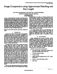
Fig. 2 depicts the file structure for our framework. Each shaded region in Fig. 2 represents the compressed data of the wire-net mesh, wires, or charts. The compressed wire-net mesh is placed in the head part of the file as an indexing structure. In the mesh information part, we store the auxiliary information for decoding, such as a bounding box, quantization numbers, and so on. The pointer table keeps track of the positions in the file at which the compressed data of wires and charts are stored. With a compressed mesh file, the decoding stage can be summarized as follows; •
•
wire-net mesh loading and decoding: We first restore and keep the wire-net mesh in the main memory. The mesh information and the pointer table are also read into the main memory. For each edge of the wire-net mesh, an edge-id is assigned and used as the pointer to access the corresponding wire in the compressed file. The mapping from a face to a chart is handled with a face-id in the same way. The compressed data of wires and charts can be kept either incore or out-of-core depending on the application and the data size. decompressed part selection: The desired parts to be decompressed are specified by designating some faces of the
4
Wire-net mesh
Mesh information: Bounding box Quantization bits Quantization range Etc.
Mesh information Wire/Chart ptr. table Wire #1 Wire #2
……
Wires
Wire #m Chart #1 Chart #2
Compressed geometry data Quantized normal vector Compressed chart data: Compressed connectivity data Compressed geometry data
……
Charts
Compressed wire data:
Chart #n
Fig. 2.
File structure of compressed mesh data
wire-net mesh with a user input or a criterion determined by the application. • chart decoding: For the selected faces of the wire-net mesh, we first decompress the wires corresponding to the edges of the faces. Then, the chart interiors are decompressed to complete the reconstructed patches (see Fig. 1). The second and third steps are repeated when different mesh parts are required to be decompressed for processing. At that time, the decompressed data for the current parts can be stored at a cache structure for later use. In some applications, we need to traverse mesh elements in different charts across wires, instead of directly indexing wirenet mesh faces. In our implementation, the boundary faces of a restored chart contain the corresponding face- and edge-ids of the wire-net mesh. From this information, we can simply find the charts to be restored next in the wire-net mesh using the correspondence between charts and wire-net mesh faces. D. Issues of random accessible mesh compression The performance of our RAMC framework is highly dominated by how to chartify a given mesh and how to encode each chart. Note that the sizes of a wire-net mesh and wires are relative small, hence the majority of a compressed mesh file are occupied by chart data. In Sec. IV, we present a mesh chartification method that obtains a high compression ratio as well as random accessibility. In particular, we consider explicit control of random accessibility to minimize the variance of the expected time for randomly accessing any specific primitive in the given mesh. In addition, out-of-core chartification methods are discussed to handle huge meshes. Sec. V presents the details on wire-net mesh and wire encoding. In Sec. VI, we propose a highly optimized algorithm for chart compression, which is suited for our framework. IV. M ESH C HARTIFICATION The random accessibility requires partitioning of a given mesh into several charts. Obviously, the chartification result highly influences the compression ratio. We need to carefully design the mesh chartification method so that we can obtain a high ratio in compression as well as high quality in random accessibility. Among various mesh chartification methods, we adopt the approach based on the Lloyd’s method [38], which has been known to provide good results [46], [12], [6]. In the approach, the chartification result is obtained by iterations of two steps; chart
growing and seed recomputation. For bootstrapping, we select a number of faces, each of which becomes the seed of a chart. In the chart growing step, using a cost function, each chart grows from a seed face by conquering its adjacent faces which have not been involved in any chart yet. The chart growing step is conducted until every face in the mesh is included in one of the charts. In the seed recomputation step, seed triangles are repositioned at the centroid of charts to improve the quality of the chartification in the next stage of chart growing. The final result is obtained when the chartification is not updated any more by the iterations. The key issue of this chartification algorithm is the design of the cost function used in the chart growing step, which depends on the chartification criteria for the applications. In our framework, we design the cost function to achieve the required properties for random accessible mesh compression. A. Required properties For our RAMC framework, mesh chartification should provide the following properties; • High compression ratio: Each chart will be independently encoded by a mesh compression technique. Our chartification algorithm must provide a set of charts, each of which can be encoded with a high compression ratio. • Random accessibility: If we only focus on compression efficiency in the chartification stage, then abnormally large charts may be generated. When accessing mesh primitives in such a large chart, the size of decoded data would be much larger than other charts, which worsens the I/O efficiency with longer waiting time. To prevent this problem, the random accessibility factor should be considered in chartification. • Topological problem: Since we restrict a wire-net mesh to a polygonal mesh, it would be impossible to construct a wire-net mesh if the chartification result has an improper structure among charts. We should prevent such a case in chartification. B. Cost function To achieve a high compression ratio for chart encoding, we consider two properties of charts; planarity and compactness. In general, a planar mesh can be efficiently compressed since the geometry in a planar region is highly coherent and well predictable. To enhance the encoding efficiency for charts, we make each chart as planar as possible. Besides the planarity, the shapes of charts also influence the compression efficiency. Assume that the chartification result has complex chart boundaries. Then, the number of the vertices on a wire increases, and the overall coding efficiency becomes worse because the wire vertices are inefficiently encoded due to low coherency. Moreover, the complex boundaries also worsen the compression performance for chart interiors in general. Hence, we enforce chart boundaries as compact as possible to minimize the number of vertices on wires. The cost function considering the planarity and compactness has been proposed in [46] for feature-sensitive chartification. We adopt the cost function defined by F( f ; c)
=
(λ − (Nc · N f ))(| Pf − Pn |).
(1)
In Eq. (1), F( f ; c) is the cost function for an unconquered face f , where a chart c tries to grow by conquering its adjacent face f .
5
C Cn
C Cn
(a) without R(c)
C
Ci C Ck Cn j
Case I
C1
C2C2 Ci Ci k Ck Cj CC j C1
(b) with R(c)
Fig. 3. Comparison of chartification results of the Venus model: (a) without the random accessibility term; (b) with the random accessibility term. By comparing the charts around eyes and curls, we can see that the sizes of charts in (b) are more regular than in (a).
The planarity is considered in Eq. (1) by calculating the normal variation between the average normal of the faces Nc in the chart c and the face normal N f . The compactness is reflected by the geodesic distance between the centroid Pf of face f and the centroid Pn of the face n in the chart c which is adjacent to f . The parameter λ regulates the relative weights between planarity and compactness. When λ is large, F( f ; c) is insensitive to the normal variation and the cost is dominated by the geometric distance. Therefore, the larger λ is, the more compactness and the less planarity are considered. In practice, if a chart is planar with low normal variation, then the vertex positions are well predictable and efficiently encoded. Hence, to achieve a good compression ratio, we set λ to 1, which is the minimum value for preventing negative F( f ; c). For random accessibility, any mesh parts should be accessible within an expected amount of I/O time from a compressed data. The upper-bound of access time for any primitives in a given chart is dominated by the number of faces in the chart. Therefore, to guarantee a bounded I/O time for arbitrary random accesses, we enforce the chart sizes to be well-balanced in the chartification. The random accessibility can be controlled by incorporating the term � � # fc α R(c) = (2) # favg into the cost function. In Eq. (2), # fc and # favg denote the number of faces in the current chart c and the average number of faces of all charts, respectively. We call the term R(c) the random accessibility factor, which enforce to minimize the variation of the expected I/O time by regularizing the number of primitives in each chart. The parameter α is a user-specified one. In this paper, we use 1.0 for α in the experiments. Finally, we define the cost function for our chartification, as follows; F 0 ( f ; c)
C
Ci Cj Ck Cn
=
R(c) · F( f ; c).
(3)
In Eq. (3), the term R(c) acts as a spring that pushes the chart boundary outward when chart c is small but pulls the chart boundary when c is large. To demonstrate the merit of random accessibility term R(c), we compare the chartification results with and without R(c). Fig. 3 shows the visual comparison between the chartification results from F( f ; c) and F 0 ( f ; c). We can see that the sizes of charts in the result using F 0 ( f ; c) are more regular than that using F( f ; c).
(a)
C1
C2C2 Ci Ci k Ck Cj CC j C1
C2
C1
C3
C2 Case II
C3
C1
(b)
Case III
Ci Cj Ck C3
(c)
III II Fig. Case 4. I Restrictions onCase chart topology: (a)Case island chart; (b) donut shaped chart; (c) two charts sharing two boundaries.
C. Topological problem handling In the chartification process, abnormal charts may be generated which are improper for generating a wire-net mesh. We postprocess the abnormal charts after the Lloyd’s method as follows (see Fig. 4); • An island chart is a chart fully surrounded by a single neighbor chart. The corresponding wire-net mesh face has only one edge, which is invalid for a polygonal mesh. To resolve the problem, an island chart is merged to the neighbor chart (see Fig. 4(a)). • A donut shaped chart is a chart which surrounds several neighbor charts. It cannot be represented by a disk-like polygonal face and the wire-net mesh cannot be encoded by a polygonal mesh encoder. To avoid this case, we divide a donut shaped chart into three similarly sized charts (see Fig. 4(b)). • If two faces share more than two edges, then the resulting wire-net mesh has a double edge. In this case, one chart is divided into two similarly sized charts (see Fig. 4(c)). Usually, the number of abnormal charts and their sizes are small. Consequently, the topological repair has little influence on the final chartification result. D. Out-of-core chartification for large meshes The RAMC framework in Sec. III can be applied to encoding a huge mesh which cannot fit into the main memory, if we can chartify the mesh in an out-of-core method with a small memory footprint. Choe et al. [6] introduced an out-of-core mesh chartification technique based on the Lloyd’s method, which guarantees similar qualities to the corresponding in-core algorithms [46], [12]. The main idea of [6] is that, for each local update of chartification, only one chart and its k-ring neighbors are loaded which can fit into the main memory. Unfortunately, however, the technique in [6] takes much processing time since the local updates require too frequent I/O transmission between disk and memory. When several charts are uploaded into the main memory for each local update, the local chartification is updated only once, and the resulting charts are written back to the disk in every iteration. Although such local update is good for preventing topology changes of the uploaded charts, it imposes unnecessarily high I/O overhead on out-of-core chartification in [6]. In this paper, we reduce the processing time of out-of-core chartification using a cluster-wise approach, which has a similar strategy to [22]. The basic idea is to use clusters that contain as
Ci Cj Ck C3
6
many charts as possible, where local chartification for each cluster is repeatedly updated until an equilibrium without additional I/O transmission of charts. The final chartification result is obtained by applying additional handling to the cluster boundaries. To bootstrap the algorithm, we need to construct an initial chartification in an out-of-core way. For the initial chartification, we adopt the technique proposed in [21], which is based on spatial subdivision of a mesh into partitions. To improve the initial chartification, we first obtain a clustering of charts. We construct a graph G such that each node corresponds to a chart and each edge represents the adjacency among charts. Initially, each chart corresponds to a cluster. Then, to group charts into several clusters, we recursively merge the adjacent nodes of graph G while the total data of each cluster does not exceed the main memory buffer. In the merging process, among possible candidates, adjacent clusters for which the summed data size is smallest are merged first to regularize the data sizes of final clusters. Once the clusters of charts have been obtained, we compute the optimal chartification result for each cluster with the in-core Lloyd’s method. Then, to update the chartification around the cluster boundaries, we perform the Lloyd’s method on the set of charts that are adjacent to the cluster boundaries. For further optimization, we may need additional iterations of the Lloyd’s method on the clusters of charts. However, in practice, improvement of chartification is small with this further processing, and we take the result of boundary handling as the final output of our out-of-core chartification. As shown in Table III of Sec. VII, the processing time is dramatically decreased due to the reduced data transmission, while chartification results are comparable to [6]. V. W IRE -N ET M ESH AND W IRE E NCODING Basically, a wire-net mesh is a polygonal mesh, which can be encoded with a conventional polygonal mesh encoding scheme [33], [23]. To encode the connectivity, we adopt the connectivity encoding scheme proposed by Khodakovsky et al. [33]. For geometry coding, we can consider the parallelogram prediction described in [24]. However, a wire-net mesh has more irregular distribution of vertex positions than ordinary polygonal meshes because it is constructed from a chartification result. This property worsens the compression efficiency of the parallelogram prediction. Hence, we modify the prediction to use the centers of polygons, where vertex geometry is represented by the correction vectors from the polygon center (see Fig. 5(a)). To encode a wire, we only need to encode the number of vertices and vertex positions since a wire is a sequence of vertices. For geometry encoding, we use a linear prediction for the vertex sequence, which is an 1D version of the parallelogram prediction. In Fig. 5(b), black vertices are already encoded/decoded and the white vertex is to be processed. We predict the position p0k by p0k = p j + (p j − pi ). After the prediction, we quantize the correction vector from p0k to pk . As will be discussed in Sec. VI-B, for geometry encoding of charts, the normal vector is stored for each wire to provide the local z-axis of vertices around the chart boundary. The vector is computed as the average normal vector of faces adjacent to the wire and quantized by spherical quantization described in [45]. VI. C HART E NCODING In our RAMC framework, to achieve a good compression ratio, we adapt a single-rate mesh compression scheme for chart
Pj
Pj Pi
pi
pj
pk′
pi
pj
pk
pk
Pi
(a) vertices on a wire-net mesh
pk′
(b) vertices on a wire
Fig. 5. Geometry encoding of a wire-net mesh and a wire: (a) Each vertex position in a polygon Pj of a wire-net mesh is encoded from the predicted center of Pj , which is computed from the center of polygon Pi with the parallelogram rule. (b) Each vertex position pk in a wire is encoded with the prediction p0k , which is obtained by the 1D version of the parallelogram rule with two previous vertices, pi and p j . front vertex
front face
z-axis (Normal of back face) y-axis
gate back face
(a)
x-axis
(b)
Fig. 6. Definitions for chart encoding: (a) terminology for connectivity encoding; (b) local frame for vertex position encoding.
encoding. After analyzing the required properties, we select the best suitable algorithm and highly optimize it for better coding efficiency. A. Connectivity coding There are two categories for mesh connectivity encoding; valence-based approaches [51], [2] and face-based approaches [44], [36], [31]. A valence-based technique exploits the vertex valences to encode mesh connectivity. In contrast, a face-based approach encodes mesh connectivity using symbols that differentiate the configurations of a newly visited face and the already conquered region. For connectivity coding in chart compression, we found that a face-based approach is more suitable than a valence-based one. With a valence-based approach, we have to generate two or more symbols for the valence of each vertex in chart boundaries since a boundary vertex is visited once for encoding each chart that contains the vertex. In contrast, a face-based approach utilizes faces as the encoding primitive which is not shared among charts. Among the face-based techniques, we choose Angle Analyzer [36], which shows a good compression ratio. Angle Analyzer encodes the mesh connectivity by generating a symbol per face. The faces are traversed in a deterministic order using a gate which is a directional edge dividing the conquered region and the nonconquered region (see Fig. 6). When the conquered region grows by stitching a front face of an active gate, one of five symbols is generated to indicate the configuration of the front face to the conquered region. The five symbols are CREATE, CW, CCW, JOIN , and SKIP , where JOIN and SKIP are special symbols for handling the topology change of the conquered region and the mesh boundary, respectively. We call the others regular symbols that are used for traversing mesh faces. To improve the compression ratio of charts, we adapt the connectivity encoding of Angle Analyzer in two ways.
7
Encoding Direction BtoC CtoB BtoC CtoB BtoC CtoB
Model Iphigenie Skull Igea
Regular Symbols 198,461 199,811 196,576 196,518 134,305 134,258
SKIP
JOIN
0 16,452 0 13,972 0 11,764
1,597 138 32 0 51 6
Bit Rate (bits/v) 2.168 2.291 1.226 1.620 1.818 2.277
TABLE I C OMPARISON RESULTS OF DIFFERENT ENCODING DIRECTIONS FOR CHARTS ; FROM CHART BOUNDARY TO INTERIOR (BtoC) AND FROM CENTROID OF A CHART TO BOUNDARY (CtoB). A LL MESHES ARE DIVIDED INTO 100 CHARTS .
Create
CW
2500 2000 1500 1000 500 0 0
20
40
60
80
100 120 140 160 180
Fig. 7. Distribution of connectivity symbols of Skull model with respect to the opening angles at the active gates: The x-axis is the opening angle and the y-axis is the counts of symbols. In connectivity encoding of Angle Analyzer, the majority of symbols are C REATE and CW, and only the dispersions of these symbols are shown with graphs.
1) encoding direction: There are two ways to conquer the faces of a chart; i) from the centroid to the boundary or ii) from the boundary to interior. In the first approach, since the coder has no prior information about the chart boundary, we will have many occurrences of a special symbol (i.e., SKIP) to indicate the boundary. In the second case, since the region is conquered from the chart boundary, we may need many of another special symbol (i.e., JOIN) due to the frequent topology changes of the conquered region in the traversal. Table I shows the distribution of the special symbols for connectivity coding and the corresponding compression ratios with two different encoding directions. In Table I, the number of the special symbols generated by conquering charts from the boundaries to interiors is much less than the reverse direction. In general, special symbols reduce the coherency of encoded symbols, which incurs a low compression ratio, as demonstrated in Table I. Hence, our connectivity coder conquers a chart from its boundary to the interior. In addition, this traversal direction provides natural stitching of chart faces to wires, requiring no additional information to be stored. Once the wires adjacent to a chart are restored, the faces of the chart can be restored starting from the wires. In our implementation, the edges in the wires, which are the boundary edges of the chart, constitute the initial gate list for face traversal. 2) optimizing chart connectivity coding: FreeLence [31] shows that the performance of a connectivity corder can be improved by exploiting geometric information. In [31], the symbols for free valences are relabeled according to the opening angles at the active gates, in order to optimize the coding efficiency by concentrating the symbol dispersions. Similarly, in this paper, we use the geometric information to enhance the coding efficiency
for connectivity symbols. Fig. 7 shows the tendency of the connectivity symbols of skull model with respect to the opening angles defined at active gates. To utilize such a property, we relabel the connectivity symbols according to the opening angles so that the symbol dispersion becomes more concentrated. In Fig. 7, the frequency of CW is higher than that of CREATE if the opening angle is less than 90 degree. Otherwise, CREATE appears more frequently than CW. Assume that we label the symbols with integers for encoding, such as 0 for CREATE, 1 for CW, and so on. Then, we relabel CREATE and CW as 1 and 0, respectively, when the opening angle is greater than 90 degree. The relabeled symbols can be encoded more effectively by an entropy coder because the frequencies of symbols have become more concentrated. In our experiments, almost all meshes showed similar distributions of connectivity symbols so we can predict the symbol at the active gate using the opening angle. With this prediction, we can achieve about 5-10% improvement in the compression ratio for connectivity encoding. In decoding time, the additional information for recovering the relabeled connectivity symbols is negligible. Only one integer is required to specify the opening angle that separates the tendency of the connectivity symbols. B. Geometry coding The vertex geometry is encoded by quantizing the local coordinates defined by the local frames, as in Angle Analyzer [36]. The local frames are defined as follows; x-axis is on the active gate, z-axis is the normal vector of the back face of the active gate, and y-axis is determined by the cross product of x- and z-axes (see Fig. 6(b)). When encoding vertices adjacent to a chart boundary, we cannot define the local z-axis because there are no back faces for them. To resolve such problem, we store at each wire the average normal vector of faces adjacent to the wire, and use the vector as the local z-axis for such vertices. In our experiments, the size of these additional data for normal vectors is small enough to be negligible. To efficiently compress the geometry information, we encode the quantized local coordinates with an adaptive arithmetic coder [52], which dynamically adjusts the frequency table for symbols. Usually, the frequency table is converged and stabilized after some amount of symbols have been streamed. However, if charts are small, symbol streams can be terminated before the frequency tables are stabilized. In this case, we cannot fully utilize the advantage of the adaptive arithmetic coder and the coding efficiency will become poor. To avoid such loss of coding efficiency, we use a pre-defined table which explicitly provides the initial frequencies of symbols. To provide the pre-defined table, we need one more encoding pass. Before encoding chart geometry, the frequencies of symbols in all charts of a mesh are accumulated by simulating the chart encoding. Then we forcibly initialize the frequency table of the arithmetic coder using the accumulated symbol frequencies. With this effective initial guess for the arithmetic coder, we can achieve about 20-30% improvement in geometry coding. In the decoding time, we need to initialize the same frequency table for correctly restoring charts. Hence, we explicitly store the pre-defined table in the compressed file, where only one table for the entire mesh is an ignorable overhead compared to the entire file size.
8
For a better initialization of the arithmetic coder, we can maintain one pre-defined table for each chart. However, in this case, the data size for the tables will increase, paying off the gain obtained in the arithmetic coder. In our experiments, one predefined table shared by all charts in a mesh is a good compromise of the storage overhead for the table and the gain in the arithmetic coding.
Model Feline Igea Skull Iphigenie
# of Vertices 49,864 67,180 98,306 100,023
Time for different # of 60 70 80 13.35 13.52 13.98 22.53 22.78 23.15 39.25 39.48 39.82 45.18 44.96 45.34
TABLE II T IMING STATISTICS FOR IN - CORE CHARTIFICATION NUMBERS OF CHARTS .
charts (sec) 90 100 14.4 14.83 23.72 24.37 40.23 41.28 45.92 45.49 WITH DIFFERENT
VII. E XPERIMENTAL R ESULTS All meshes used in this paper for experiments are manifold because the chart encoder can handle only manifold meshes. However, this restriction can be avoided in our RAMC framework if we adopt a chart encoder that can process non-manifold meshes. For the experiments, we use a Windows PC with a Pentium Core2 Duo 2.4GHz CPU and 2GB memory. A. Geometry quantization numbers The geometry of a wire-net mesh should be accurately represented since it provides a skeleton structure for the reconstruction of charts. We usually encode the vertex positions of a wirenet mesh with 10-12 bit global quantization, which is generally acceptable for encoding a polygonal mesh [50], [19], [24], [36], [3], [41]. When the input mesh is very large, e.g., an out-of-core mesh, we use 13-14 bits for quantizing the resulting wire-net mesh. We also carefully determine the quantization number for the geometry coding of wires because the wires are the starting points for decoding charts. The restored geometry of wires highly influences the final accuracy of the restored charts. From several experiments, we found that usually twice the quantization number used to encode the inner chart geometry is acceptable for encoding the wire geometry. To encode vertex positions of charts, we use local quantization with the local frames defined at the vertices. Similar to [36], we select the proper quantization numbers for local coordinates by comparing the distortions between the charts quantized with our local frames and the charts from 12-bit global quantization. The distortions are measured by the Metro tool [10]. Ideally, we can use different quantization for different charts. However, it is inefficient to store the quantization information per chart in the compressed mesh file. In our implementation, we measure the proper quantization range for each chart, and compute the maximum range that covers the ranges of all charts. With the range, we determine the quantization number for each chart which is compatible to 12-bit global quantization of the chart. We then compute the maximum of the quantization numbers of all charts. Finally, all charts are encoded with the same quantization range and number for local quantization. B. Chartification Table II shows the processing time of in-core chartification with different numbers of charts. For small meshes, we obtain the initial chartification by face clustering [16] for better results. After the initial chartification, we iterate the seed recomputation and chart growing steps of the Lloyd’s method five times. In general, five times of iterations may not achieve the optimal results but as described in [12], near-optimal results can be obtained, which are good enough for our RAMC framework. Table II shows that the processing time is proportional to the number of vertices in
(a)
(b)
(c)
Fig. 8. Chartification results of huge meshes and their wire-net meshes: (a) Dragon; (b) Buddha; (c) Lucy
a mesh. The number of charts to be generated also affect the processing time. Table III shows the timing results of our out-of-core chartification for large meshes. Fig. 8 shows the chartification results. The input meshes are represented by the indexed mesh format. During the out-of-core chartification, the intermediate data are saved in disk as two files per a chart; one is a sub-mesh data which is represented by an indexed mesh and the other keeps the global vertex indices used to stitch charts seamlessly. The sum of the intermediate file sizes is a little larger than the original mesh data. The amounts of required memory and data transmission depend on the sizes of chart clusters that are loaded into memory for the iterations of the Lloyd’s method. The sizes can be easily controlled in the chart clustering step described in Sec. IV-D. For all experiments in this paper, we used the vertex buffer that can take one million vertices, while the face buffer can take two million faces. Similar to the in-core chartification, we perform five iterations of the seed recomputation and chart growing for each chart cluster and the charts along cluster boundaries. C. Compression ratio Table IV shows the compression ratio of our RAMC framework. The second column gives the number of charts and the average number of faces in a chart for each experiment. The third column shows the size of overhead information that includes the wire-net mesh for random accessibility and essential data for
9
Model Dragon Buddha xyzrgb Dragon Lucy
# of Vertices 400,000 541,366 3,609,455 14,027,867
# of Charts 273 584 576 1,195
Initial Chartification 5m 9s 6m 50s 1h 55m 3h 15m
Chart update [6] ours 7m 6s 30s 6m 51s 6m 30s 1h 20m 37m 6h 33m 2h 25m
Compression 30s 40s 5m 50s 28m
TABLE III T IMING STATISTICS FOR COMPRESSING LARGE MESHES WITH OUT- OF - CORE CHARTIFICATION : F OR COMPARISON OF CHART UPDATE TIME WITH [6], A GIVEN MESH IS CHARTIFIED INTO THE SAME NUMBER OF CHARTS .
Model Feline
Igea
Skull
Iphigenie
Dragon Buddha xyzrgb Dragon Lucy
# of Charts (Avg # of F) 50 (1,995) 60 (1,662) 70 (1,425) 80 (1,247) 90 (1,108) 100 (997) 50 (2,687) 60 (2,239) 70 (1,919) 80 (1,679) 90 (1,493) 100 (1,343) 50 (3,932) 60 (3,277) 70 (2,809) 80 (2,458) 90 (2,185) 100 (1,966) 60 (3,334) 70 (2,858) 80 (2,501) 90 (2,223) 100 (2,001) 273 (2,930) 584 (1,854)
Overhead (bits/v) 0.72 0.89 0.95 1.05 1.14 1.18 0.46 0.54 0.61 0.66 0.75 0.84 0.36 0.36 0.43 0.51 0.51 0.57 0.43 0.52 0.58 0.59 0.68 0.34 0.50
Wire (bits/v) 1.69 1.92 2.01 2.14 2.31 2.35 1.32 1.48 1.63 1.71 1.82 2.01 1.14 1.14 1.23 1.39 1.39 1.54 1.34 1.52 1.62 1.59 1.70 1.77 2.37
576 (12,532)
0.07
0.85
7.63
8.55
1195 (23,478)
0.04
0.69
13.91
14.65
TABLE IV C OMPRESSION RESULTS USING THE RAMC
Chart (bits/v) 14.30 14.69 14.30 13.69 14.50 14.14 14.27 14.47 14.56 14.30 14.56 14.63 10.76 10.43 10.57 10.98 10.83 10.80 12.33 12.33 12.03 12.47 12.99 14.83 16.19
FRAMEWORK :
Total (bits/v) 16.71 17.51 17.26 17.15 17.95 17.67 16.05 16.49 16.81 16.67 17.14 17.48 12.26 11.94 12.23 12.88 12.73 12.91 14.10 14.37 14.23 14.65 15.37 16.94 19.06
T HE BIT RATIO
OF EACH COMPONENT IS COMPUTED BY DIVIDING THE DATA SIZE OF THE COMPONENT BY THE TOTAL NUMBER OF VERTICES IN THE MESH .
decoding, such as quantization numbers and the pre-defined table. The fourth column shows the bit-rate for the wires, which includes the numbers of vertices in wires, wire geometry data, and average gate normals. The fifth column is the bit-rate for charts which comes from the encoded data of chart connectivity and geometry. As shown in Table IV, when the number of charts becomes larger, the overhead to provide random accessibility increases because the wire-net mesh becomes more complicated and more vertices are included in wires. However, for reasonable numbers of charts which correspond to the chart sizes ranging from 1,000 to 23,000 faces, the overhead remains small compared to the entire data size. In Fig. 9, the compression ratios of the RAMC framework with different numbers of charts are compared with those of other mesh compression techniques, such as single-rate compression [51], [36] and progressive compression [1]. The encoders of [51], [1] were obtained from the web pages of the authors. For [36], we used our own implementation. We used 12-bit global quantization
Fig. 9. Comparison of the compression ratio with other compression schemes: TG and AA are from single-rate compression algorithms, [51] and [36], respectively. PME is the result of a progressive mesh encoder [1].
to encode geometry for [51] and [1]. In the case of [36], we found the quantization numbers for the local coordinates which have the same distortion errors with 12-bit global quantization. Fig. 9 demonstrates that our RAMC framework has only a little worse compression ratios than other schemes, while providing the decent property of random accessibility. Besides the methods covered in Fig. 9, the encoders of [31] and [42] achieve the best performances in the single-rate and progressive mesh compression domains, respectively. However, the softwares for the encoders are not publicly available and we have not directly compared the compression ratio with them. Instead, we use the results from the reports in [31] and [42]. In [31], the compression results are about 27% better than Angle Analyzer and in [42], the gain is about 10-30% improvement over [1] for irregular meshes. From these facts, we can infer that our compression results are still comparable with the state-of-the-art techniques in single-rate and progressive mesh compression. We also compare our compression results for large meshes with out-of-core compression techniques [21], [25]. However, in this case, we cannot directly compare the compression ratios, because we encode the geometry of charts using local frames while vertex positions of the entire mesh are encoded with global quantization in [21], [25]. For a large mesh, the bounding boxes of charts are much smaller than that of the entire mesh. Consequently, for the same amount of geometric distortion, the global quantization bits needed for the entire mesh is larger than those for charts. Since the local frames for charts are quantized to be compatible with 12-bit global quantization of the biggest chart, we can approximate the quantized cell size of charts by dividing the bounding box size of the biggest chart by 212 . Then, using the bounding box of the whole mesh, we can estimate the global quantization bits that are
10
Model Dragon Buddha xyzrgb Dragon Lucy
Global Quantization Bits (14,14,14) (13,14,13) (15,14,15) (14,13,15)
TABLE V G LOBAL QUANTIZATION BITS FOR THE WHOLE MESH WHICH CORRESPOND TO 12- BIT QUANTIZATION OF THE BIGGEST CHART: E ACH TRIPLE CONTAINS THE NUMBERS OF BITS FOR x, y, AND z AXES .
needed for a similar quantized cell size for the entire mesh. Table V shows the estimated global quantization bits for large meshes, which are 13-15 bits in our experiments. In [21], [25], the compression results for large meshes are about 10-25 bits/v with 16-bit global quantization. Particulary in [25], 16.48 bits/v for Lucy and 24.22 bits/v for Buddha were reported. Table IV shows 14.65 bits/v for Lucy and 19.06 bits/v for Buddha. Although our results are compatible with 13-15 bit global quantization, the improvements in the compression ratios are about 2-5 bits/v, similar to or more than the differences in the global quantization bits. These comparisons imply that our technique is comparable to previous out-of-core compression techniques in the compression ratios, while providing the random accessibility for decoding. Note that for large meshes, the size of the overhead information in our RAMC framework is relatively small to the mesh data and has little influence on the compression ratios.
D. Chart decoding time Table VI shows the chart restoration time for large meshes. We can see that the time is almost linear with respect to the number of faces in a chart. We test two traversal strategies during encoding/decoding of charts; one is Geometry Guided which is used in our framework, and the other is Sequential Traversal. The former focuses on a better compression ratio and the traversal order is determined by the mesh geometry, as in [36], [31]. However, in this case, the encoder/decoder should search the active gate from the gate list using geometry information, and the search slows down the decoding speed. In contrast, the Sequential Traversal strategy uses the front of the gate list for the active gate without any search, so the encoding/decoding can be performed fast. However, in this case, we have a loss of compression ratio of about 1.5-2.5 bits/v for connectivity. Therefore, between the two strategies, there is a trade-off among the compression efficiency and chart decoding speed. In Table VI, we also compare the chart restoration times between the compressed and uncompressed data. In recent computer systems, the CPU power and memory capacity have increased rapidly but the data transmission speed between disk and main memory cannot catch up with such improvements and can become a bottleneck. Hence, we can enhance the processing speed for large meshes by decreasing the amount of transmitted data. Table VI shows that our RAMC framework has potentials for such enhancement, especially with the Sequential Traversal strategy, in addition to reducing the disk space for storing large meshes. Our current implementation focuses on the compression ratio rather than the speed and uses chart encoding with geometry information. If necessary for applications, we can speed up the
Fig. 10. Out-of-core rendering of Lucy: The yellow mesh is the wire-net mesh, which shows the rough shape of the original mesh. The black cube is the view frustum and charts intersecting the cube are restored and rendered.
chart decoding by encoding chart data with an algorithm which offers faster decoding, such as [51], [29]. E. Applications The RAMC framework can be used for several applications, such as rendering, smoothing, and editing. It can provide a general underlying structure for processing large meshes in an out-of-core manner. 1) Out-of-core rendering: Out-of-core rendering for large meshes is an intuitive application of the RAMC framework. Most of mesh data can be reserved in the disk in the compressed form while only the system-requested charts are restored in the main memory. With this approach, we can reduce the overhead occurred by restoring the unnecessary parts of the mesh. Fig. 10 shows an example of out-of-core rendering. We only decode the charts which intersect the view-frustum illustrated as the black cube. When some charts escape from the viewfrustum, they are released from the main memory. Such dynamic load/release of charts enables us to enhance the memory usage and render huge meshes with small memory footprint. 2) Out-of-core mesh smoothing: Fig. 11 shows an example of partial smoothing of the Lucy model. We load charts corresponding to the face of Lucy into main memory and perform Laplacian smoothing 100 times. Due to the random accessibility, we can re-encode the smoothed mesh part without touching other parts of the mesh. In Fig. 11(a), the original compression rate of selected parts is 14.47 bits/v. The compression rate changes to 9.98 bits/v after the smoothing in Fig. 11(b). This result is natural because Laplacian smoothing reduces the entropy of the geometry and enhances the compression efficiency. Besides the partial smoothing, we can smooth the entire mesh by traversing and smoothing the charts one by one. 3) Out-of-core mesh editing: Fig. 12 shows an example of out-of-core editing. Similar to the case of smoothing, we load the charts for the face of Lucy and stretch the nose. After the editing, we re-encode the modified part. The average bitrate of selected parts has changed to 15.02 bits/v after editing. The editing operation makes the geometry more complicated and reduces the coding efficiency. If re-encoding of a modified mesh part needs more bits than the original, then the file structure in Fig. 2 does not allow us to save the part back to the same position in the compressed file. To simplify the process of saving re-encoded mesh parts, we can
11
Models
# of Charts
Dragon Buddha xyzrgb Dragon Lucy
273 584 576 1,195
Average Chart Decoding Time Geometry Sequential Avg # of F Uncomp. Guided Traversal 2,930 0.023 s 0.009 s 0.025 s 1,854 0.011 s 0.006 s 0.007 s 12,532 0.062 s 0.032 s 0.058 s 23,478 0.274 s 0.099 s 0.083 s
Maximum Chart Decoding Time Geometry Sequential # of F Uncomp. Guided Traversal 15,653 0.078 s 0.062 s 0.093 s 5,648 0.047 s 0.032 s 0.047 s 43,352 0.219 s 0.140 s 0.359 s 87,842 1.547 s 0.422 s 1.359 s
TABLE VI T IMING STATISTICS FOR CHART RESTORATION OF LARGE MESHES .
(a)
(b)
Fig. 11. Out-of-core smoothing for Lucy: (a) Before smoothing; (b) After performing Laplacian smoothing 100 times. The average bit rate for the loaded wires and charts is 14.47 bits/v. After smoothing, we re-encode the smoothed parts and the bit-rate is 9.98 bits/v, because a smooth surface can be compressed more efficiently.
(a)
(b)
Fig. 12. Out-of-core editing for Lucy: (a) Before editing; (b) After editing, the nose of Lucy has been stretched. The loaded wires and charts are the same as the case of smoothing. After editing, the edited part is re-encoded with 15.02 bits/v, because such an editing reduces the regularity of vertex positions.
store the wire and chart data as multiple files in disk; one file per each wire and one file per each chart. In this case, we do not need to maintain the wire/chart pointer tables in Fig. 2 since we can easily identify wire/chart files with a naming convention using the edge-id and face-id of the wire-net mesh. VIII. D ISCUSSION
AND
C ONCLUSION
A. Comparison with other techniques Octree-based External Memory Mesh (OEMM) framework [9] was proposed to manipulate large meshes with small memory footprints. By constructing an octree structure, OEMM enables handling a large mesh on a low-end system, where mesh parts can be loaded into memory for processing while others remain in disk. This property is similar to random accessibility of our framework. However, OEMM uses a raw format for accessing partial meshes and storing mesh data in disk. This approach would be convenient for manipulating mesh data but requires more disk space than our framework. In addition, our framework uses a wire-net mesh that provides a natural and efficient stitching structure for randomly accessed mesh parts, while OEMM needs additional operations
for the triangles crossing octree cell boundaries to find the vertices in neighbor cells. Kim et al. [35] proposed a framework for multiresolution random accessible mesh compression (MRAMC), in which portions of a mesh can be decompressed in desired resolutions without decoding other non-interesting parts. The main advantage of the technique is that it can provide a coarse-to-fine style of decompression, which is difficult to accomplish in random accessible compression. However, the cost for geometry coding is high because the static information of vertex neighbors cannot be utilized in the decoding stage. Compared to our RAMC framework, MRAMC has a trade-off among multiresolution restoration and a high compression ratio. The progressiveness of MRAMC would be useful for rendering or transmission of large meshes via networks in a compressed format. In contrast, RAMC would be more suitable for memory efficient processing of large meshes in a local machine. Recently Yoon et al. [53] proposed a compressed mesh format that supports random order access to the compressed data in run time. Their technique divides a cache-oblivious layout [54] of a mesh into the same-sized blocks and each block is separately encoded using the streaming mesh compression algorithm [29]. The technique preserves the order of mesh elements in encoding, which is good for some applications but hinders optimizing the compression ratio. Consequently, the compression ratios are worse than our RAMC framework. In addition, the technique only supports read-only access, whereas our framework can handle local modification of mesh parts. B. Summary and future work In this paper, we presented a framework for random accessible mesh compression and its applications. Due to random accessibility, we can partially restore only the necessary mesh parts from the compressed data. The wire-net mesh provides a structure for indexing necessary parts and stitching separately decoded parts. To achieve a good compression ratio, we adapt a single-rate mesh encoding technique and optimize it for our framework. To support random accessibility more effectively, we consider the regularity of chart sizes which bounds the amount of I/O transmission by avoiding abnormally large charts. We apply the RAMC framework to several applications, such as out-ofcore rendering, smoothing, and editing. In the applications, we can perform geometric operations on mesh parts and write back the modification to disk without touching other parts due to the random accessibility. When we re-encode an edited mesh part with excessive changes of vertex positions, new vertex coordinates defined by local frames may escape out of the quantization range for charts. In
12
this case, we store the expanded quantization range for the edited chart. Although this expansion of the quantization range incurs more distortions of the chart than before editing, for simplicity, in our implementation, we use the same quantization number for the chart. If excessive and repeated editing operations are required with high precision positions, then a possible solution is to use lossless compression of predicted floating-point numbers for mesh geometry [28]. In our RAMC framework, a single-rate algorithm is used for encoding charts to achieve a better compression ratio. It is interesting future work to incorporate progressive chart encoding into the framework so that we can control the amount of details in the decoded mesh parts. ACKNOWLEDGMENTS The ‘dragon’, ‘happy buddha’, ‘xyz rgb dragon’, and ‘lucy’ models are courtesy of Stanford Computer Graphics Lab. The ‘skull’ model is courtesy of Headus (www.headus.com.au) and Phil Dench. The ‘Igea’ and ‘dinosaur’ models are courtesy of Cyberware. The ‘feline’ model is courtesy of Multi-Res Modeling Group at Caltech. The ‘Iphigenie’ model is courtesy of Computer Graphics & Multimedia Group at RWTH Aachen. R EFERENCES [1] P. Alliez and M. Desbrun, “Progressive encoding for lossless transmission of 3D meshes,” Proc. ACM SIGGRAPH 2001, pp. 298–205, 2001. [2] ——, “Valence-driven connectivity encoding of 3D meshes,” Computer Graphics Forum (Proc. Eurographics 2001), pp. 480–489, 2001. [3] P. Alliez and C. Gotsman, “Recent advances in compression of 3D meshes,” Advances in Multiresolution for Geometric Modeling, pp. 3– 26, 2005. [4] M. Attene, B. Falcidieno, M. Spagnuolo, and J. Rossignac, “Swingwrapper: Retiling triangle meshes for better edgebreaker compression,” ACM Trans. Graphics, vol. 22, no. 4, pp. 982–996, 2003. [5] C. Bajaj, I. Ihm, and S. Park, “3D RGB image compression for interactive applications,” ACM Trans. Graphics, vol. 20, no. 1, pp. 10– 38, 2000. [6] S. Choe, M. Ahn, and S. Lee, “Feature sensitive out-of-core chartification of large polygonal meshes,” Proc. Computer Graphics International 2006, pp. 518–529, 2006. [7] S. Choe, J. Kim, H. Lee, S. Lee, and H.-P. Seidel, “Mesh compression with random accessibility,” Proc. the fifth Israel-Korea Binational Conference on Geometric Modeling and Computer Graphics, pp. 81–86, 2004. [8] P. Cignoni, F. Ganovelli, E. Gobbetti, F. Marton, F. Ponchio, and R. Scopigno, “Adaptive tetrapuzzles: Efficient out-of-core construction and visualization of gigantic multiresolution polygonal models,” ACM Trans. Graphics (Proc. ACM SIGGRAPH 2004), vol. 23, no. 3, pp. 796– 803, 2004. [9] P. Cignoni, C. Montani, C. Rocchini, and R. Scopigno, “External memory management and simplification of huge meshes,” IEEE Trans. Visualization and Computer Graphics, vol. 9, no. 4, pp. 525–537, 2003. [10] P. Cignoni, C. Rocchini, and R. Scopigno, “Metro: Measuring error on simplified surfaces,” Computer Graphics Forum, vol. 17, no. 2, pp. 167– 174, 1998. [11] D. Cohen-Or, D. Levin, and O. Remez, “Progressive compression of arbitrary triangular meshes,” Proc. IEEE Visualization ’99, pp. 67–72, 1999. [12] D. Cohen-Steiner, P. Alliez, and M. Desbrun, “Variational shape approximation,” ACM Trans. Graphics (Proc. ACM SIGGRAPH 2004), vol. 23, no. 3, pp. 905–914, 2004. [13] M. Deering, “Geometry compression,” Proc. ACM SIGGRAPH 1995, pp. 13–20, 1995. [14] O. Devillers and P.-M. Gandoin, “Geometric compression for interactive transmission,” Proc. IEEE Visualization 2000, pp. 319–326, 2000. [15] P.-M. Gandoin and O. Devillers, “Progressive lossless compression of arbitrary simplicial complexes,” ACM Trans. Graphics (Proc. ACM SIGGRAPH 2002), vol. 21, no. 3, pp. 372–379, 2002.
[16] M. Garland, A. Willmott, and P. S. Heckbert, “Hierarchical face clustering on polygonal surfaces,” Proc. 2001 ACM Symposium on Interactive 3D Graphics, pp. 49–58, 2001. [17] E. Gobbetti and F. Marton, “Far voxels: A multiresolution framework for interactive rendering of huge complex 3D models on commodity graphics platforms,” ACM Trans. Graphics (Proc. ACM SIGGRAPH 2005), vol. 24, no. 3, pp. 878–885, 2005. [18] C. Gotsman, “On the optimality of valence-based connectivity coding,” Computer Graphics Forum, vol. 22, no. 1, pp. 99–102, 2003. [19] C. Gotsman, S. Gumhold, and L. Kobbelt, “Simplification and compression of 3D meshes,” in Tutorials on Multiresolution in Geometric Modeling. Springer, 2002. [20] X. Gu, S. J. Gortler, and H. Hoppe, “Geometry images,” ACM Trans. Graphics (Proc. ACM SIGGRAPH 2002), vol. 21, no. 3, pp. 355–361, 2002. [21] J. Ho, K.-C. Lee, and D. Kriegman, “Compressing large polygonal models,” Proc. IEEE Visualization 2001, pp. 357–362, 2001. [22] H. Hoppe, “Smooth view-dependent level-of-detail control and its application to terrain rendering,” Proc. IEEE Visualization ’98, pp. 35–42, 1998. [23] M. Isenburg, “Compressing polygon mesh connectivity with degree duality prediction,” Proc. Graphics Interface 2002, pp. 161–170, 2002. [24] M. Isenburg and P. Alliez, “Compressing polygon mesh geometry with parallelogram prediction,” Proc. IEEE Visualization 2002, pp. 141–146, 2002. [25] M. Isenburg and S. Gumhold, “Out-of-core compression for gigantic polygon meshes,” ACM Trans. Graphics (Proc. ACM SIGGRAPH 2003), vol. 22, no. 3, pp. 935–942, 2003. [26] M. Isenburg and P. Lindstrom, “Streaming meshes,” Proc. IEEE Visualization 2005, pp. 231–238, 2005. [27] M. Isenburg, P. Lindstrom, S. Gumhold, and J. Snoeyink, “Large mesh simplification using processing sequences,” Proc. IEEE Visualization 2001, pp. 465–472, 2003. [28] M. Isenburg, P. Lindstrom, and J. Snoeyink, “Lossless compression of predicted floating-point geometry,” Computer-Aided Design, vol. 37, no. 8, pp. 869–877, 2004. [29] ——, “Streaming compression of triangle meshes,” Proc. 2005 Eurographics Symposium on Geometry Processing, pp. 111–118, 2005. [30] M. Isenburg and J. Snoeyink, “Face fixer: Compressing polygon meshes with properties,” Proc. ACM SIGGRAPH 2000, pp. 263–270, 2000. [31] F. Kalberer, K. Polthier, U. Reitebuch, and M. Wardetzky, “Freelence - coding with free valences,” Computer Graphics Forum (Proc. Eurographics 2005), pp. 469–478, 2005. [32] Z. Karni and C. Gotsman, “Spectral compression of mesh geometry,” Proc. ACM SIGGRAPH 2000, pp. 279–286, 2000. [33] A. Khodakovsky, P. Alliez, M. Desbrun, and P. Schroder, “Near-optimal connectivity encoding of 2-manifold polygon meshes,” Graphical Models, vol. 64, no. 3-4, pp. 147–168, 2002. [34] A. Khodakovsky, P. Schroder, and W. Sweldens, “Progressive geometry compression,” Proc. ACM SIGGRAPH 2000, pp. 271–278, 2000. [35] J. Kim, S. Choe, and S. Lee, “Multiresolution random accessible mesh compression,” Computer Graphics Forum (Proc. Eurographics 2006), pp. 323–331, 2006. [36] H. Lee, P. Alliez, and M. Desbrun, “Angle analyzer: A triangle-quad mesh codec,” Computer Graphics Forum (Proc. Eurographics 2002), pp. 383–392, 2002. [37] P. Lindstrom, “Out-of-core construction and visualization of multiresolution surfaces,” Proc. 2003 ACM Symposium on Interactive 3D Graphics, pp. 93–102, 2003. [38] S. Lloyd, “Least square quantization in PCM,” IEEE Trans. Information Theory, vol. 28, pp. 129–137, 1982. [39] J. L. Mitchell, W. B. Pennebaker, C. E. Fogg, and D. J. Legall, Mpeg Video: Compression Standard (Digital Multimedia Standards Series). Kluwer Academic Publishers, 1996. [40] R. Pajarola and J. Rossignac, “Compressed progressive meshes,” ACM Trans. Graphics, vol. 6, no. 1, pp. 79–93, 2000. [41] J. Peng, C.-S. Kim, and C.-C. J. Kuo, “Technologies for 3D mesh compression: A survey,” Journal of Visual Communication and Image Representation, pp. 688–733, 2005. [42] J. Peng and C.-C. J. Kuo, “Geometry-guided progressive lossless 3D mesh coding with octree (OT) decomposition,” ACM Trans. Graphics (Proc. ACM SIGGRAPH 2005), vol. 24, no. 3, pp. 609–616, 2005. [43] D. Poulalhon and G. Schaeffer, “Optimal coding and sampling of triangulations,” Algorithmica, vol. 46, no. 3-4, pp. 505–527, 2004. [44] J. Rossignac, “Edgebreaker : Connectivity compression for triangle meshes,” IEEE Trans. Visualization and Computer Graphics, vol. 5, no. 1, pp. 47–61, 1999.
13
[45] S. Rusinkiewicz and M. Levoy, “Qsplat: A multiresolution point rendering system for large meshes,” Proc. ACM SIGGRAPH 2000, pp. 343– 352, 2000. [46] P. V. Sander, Z. J. Wood, S. J. Gortler, J. Snyder, and H. Hoppe, “Multi-chart geometry images,” Proc. 2003 Eurographics Symposium on Geometry Processing, pp. 157–166, 2003. [47] E. Shaffer and M. Garland, “A multiresolution representation for massive meshes,” IEEE Trans. Visualization and Computer Graphics, vol. 11, no. 2, pp. 139–148, 2005. [48] O. Sorkine, D. Cohen-Or, and S. Toledo, “High-pass quantization for mesh encoding,” Proc. 2003 Eurographics Symposium on Geometry Processing, pp. 41–51, 2003. [49] G. Taubin, A. Gueziec, W. Horn, and F. Lazarus, “Progressive forest split compression,” Proc. ACM SIGGRAPH 1998, pp. 123–132, 1998. [50] G. Taubin and J. Rossignac, “3D geometry compression,” ACM SIGGRAPH 1999 Course on 3D Geometry Compression, 1999. [51] T. Touma and C. Gotsman, “Triangle mesh compression,” Proc. Graphics Interface ’98, pp. 26–34, 1998. [52] F. Wheeler, “Adaptive arithmetic coding source code,” 1996, http://www.cipr.rpi.edu/˜wheeler/ac. [53] S.-E. Yoon and P. Lindstrom, “Random-accessible compressed triangle meshes,” IEEE Trans. Visualization and Computer Graphics (Proc. IEEE Visualization 2007), vol. 13, no. 6, pp. 1536–1543, 2007. [54] S.-E. Yoon, P. Lindstrom, V. Pascucci, and D. Manocha, “Cacheoblivious mesh layouts,” ACM Trans. Graphics (Proc. ACM SIGGRAPH 2005), vol. 24, no. 3, pp. 886–893, 2005.