Feb 20, 1992 - Alan Garvey. Marty Humphrey. Victor Lesser ..... performing different approximation algorithms, such as âlevel-hoppingâ (skip- ping some of the ...
Real-Time Control of Approximate Processing 1 Keith Decker
Alan Garvey Marty Humphrey Victor Lesser Department of Computer Science University of Massachusetts COINS Technical Report 91–50 February 20, 1992
Abstract Approximate processing is an approach to real-time AI problem solving in domains in which compromise is possible between the resources required to generate a solution and the quality of that solution. It is a satisficing approach in which the goal is to produce acceptable solutions within the available time and computational resource constraints. Previous work has shown how to integrate approximate processing with the blackboard architecture[17]. However, in order to solve real-time problems with hard deadlines using a blackboard system, we need to have: (1) a predictable blackboard execution loop, (2) a representation of the set of current and future tasks and their estimated durations, and (3) a model of how to modify those tasks when their deadlines are projected to be missed, and how the modifications will affect the task durations and results. This paper describes four components for achieving these goals in an approximate processing blackboard system. A parameterized low-level control loop allows predictable knowledge source execution, multiple execution channels allow dynamic control over the computation involved in each task, a meta-controller allows a representation of the set of current and future tasks and their estimated durations and results, and a real-time blackboard scheduler monitors and modifies tasks during execution so that deadlines are met. An example is given that illustrates how these components work together to construct a satisficing solution to a time-constrained problem in the Distributed Vehicle Monitoring Testbed (DVMT). A brief sketch is given of the implementation of the system.
1
Authors are listed in alphabetical order. This work was partly supported by the Office of Naval Research under a University Research Initiative grant number N00014-86-K-0764, NSF contract CDA 8922572, and ONR contract N00014-89-J-1877.
1 Introduction Approximate processing is an approach to real-time AI problem solving in which the system reasons about tradeoffs between the time required to generate a solution and the quality of that solution in terms of completeness, precision, and certainty. The system attempts to generate the best possible solution in the allowed amount of time. An alternate method for real-time AI problems is the class of algorithms called anytime algorithms[6]. Anytime algorithms are a subclass of approximate processing algorithms that can be terminated anytime and produce answers that improve monotonically as the time allowed increases. In contrast, approximate processing algorithms produce an answer anytime after a given deadline and produce monotonically better answers as the deadline is extended. That is, approximate processing systems take advantage of all the time available to them to generate a solution, rather than always having one at hand. Approximate processing works best in domains where deadlines can be accurately estimated and where the system has sufficient advanced notice when either a deadline will be sooner than expected, or priorities or resource constraints have changed (probably because of an increased workload) making the deadline unachievable under the current configuration. When these criteria are not met, approximate processing may not generate any solution. Approximate processing requires the problem solver to be very flexible in its ability to represent and efficiently implement a variety of processing strategies. With minimal overhead, the problem solver should dynamically respond to the current situation by altering its operators and state space abstraction to produce a range of acceptable answers[8, 17]. To achieve these goals in a blackboard system requires three key modifications. First, the opportunism inherent in the blackboard system must be balanced by the need for predictability. Hard deadlines require bounded, predictable task times and may require opportunistic responses to be tightly controlled to meet the deadlines. However, opportunistic behavior is desireable and should be encouraged in those situations when the time available allows it. The second modification involves the explicit representation of multiple reasoning activities, modes of response, and resource utilization. While the traditional blackboard model of independent knowledge sources is still useful, careful records must be kept of how the instantiated knowledge sources (the lowest level schedulable task unit) relate to the problem solving goals, what types of approximations are required, and what resources (primarily computational resources) will be required. Finally, when a deadline cannot be met using the current schedule, the schedule must be rearranged, using a combination of techniques including postponing tasks and forcing them to use faster approxi-
1
mations. The system must keep track of the new schedule, task durations, and the effect of the new schedule on the results of problem-solving. The entire real-time problem-solving architecture is shown in Figure 1. In order to provide for more predictable execution of tasks we use a parameterized low-level control loop. This extension of the traditional blackboard control loop allows the system to dynamically control how much opportunism is permitted within each task. This is accomplished by controlling the characteristics of the data that will be processed, the type of knowledge that will be applied to this data, and the granularity of the processing. Tightly constrained tasks (in terms of their inputs, outputs, and processing algorithm) are as predictable as possible without modification of the underlying operating system. Timing models, based on these constraints, allow the real-time scheduler to make accurate duration estimations. The ability to dynamically modify the low-level control loop is an extension of ideas developed originally in BB1 for dynamically specifying the predicates used to evaluate activities on the agenda in order to impose different high-level strategies[12]. We extend the ideas in BB1 by allowing a richer set of parameters (filters, mappings, and mergings, as well as heuristics) to be dynamically adjusted. Recent work by B. Hayes-Roth[2, 13] has also gone to a more complex low-level control loop that has additional parameters. The idea of dynamically adapting filters on input data for real-time systems has also been discussed in [21]; we tie this filtering into the problem of balancing predictability and opportunism. The low-level control loop is discussed in detail in Section 3.1. The second component of our architecture is channels, which allow different processing strategies to be used simultaneously. A channel is a replication of the low-level control loop for a concurrent task. Having multiple channels allows multiple processing strategies to occur simultaneously, and potentially asynchronously or in parallel[7], while still providing predictable execution. The RT-1 real-time blackboard architecture[9] used a fixed set of priority channels to partition problem-solving by event priority; in contrast, we dynamically create task channels to partition problem-solving by task. This allows us to clearly decide which problem-solving resources to devote to each task1 . Section 3.2 describes channels in more detail. With these low-level architectural concerns satisfied, the next problem is the smooth operation of the system. Control in blackboard architectures that integrate multiple reasoning methods has traditionally been accomplished through the implicit or explicit construction of an agenda rating function that allows the scheduler to choose the “best” knowledge source instance (KSI) to execute 1 A fixed set of priority channels could be built on our task channels by combining preallocated channels (one for each priority) with heuristics that rated KSIs on their channel appropriately.
2
Track Vehicle Goal System Goal
Identify Possible Pattern Goal
Control Goals Find New Vehicles Goal
Control Plan
Find New Vehicles Focus Goal Directed Strategy Identify Possible Patterns Focus
Channel 1
Channel 2
KSI Execution
KSI agenda KSI Merging Run Preconditions
Goal-to-KS mapping
Hyp blackboard Subgoaling
KSI Execution
KSI agenda KSI Merging
Hypothesis Filter Goal Filter
Run Preconditions
Hyp-to-goal mapping
Hyp blackboard
Goal Merging Goal-to-KS mapping
Goal blackboard
Execute Control KSI
Subgoaling Hypothesis Filter
Goal Filter
Hyp-to-goal mapping Goal Merging
Goal blackboard
Events Choose a Control KSI
Ratings
KSI 15
Domain KSI Agenda
Agenda Maintenance
KSI 12 KSI 23 KSI 14
Meta-Controller
KSI 19
Channelized Low-Level Loop Initial Task Set Task 1
Approximate Tasks 1 and 2 Move Task 2 to next sensor cycle
Task 1
Task 2
Task 2
Task 1
Task 2
Sensor Cycle
Real-Time Scheduler Figure 1: The real-time blackboard architecture. Each part of this architecture is explained in more detail in the Section 3. It consists of a channelized low-level loop that does domain problem-solving in multiple channels with a shared domain KSI agenda, guided by control plan and goal elements; a meta-controller that executes a control KSI loop that constructs the control plan and goals, and modifies the parameters of the low-level loop; and, a real-time scheduler that ensures real-time performance by monitoring problem-solving at the channel-task level and fixing schedules that go over time. The real-time scheduler constructs future schedules based on projected channel tasks and fills in those channel tasks with domain KSIs as the KSIs appear on the agenda. The dashed lines between modules indicate points of interaction.
3
[3, 12, 14]. A significant amount of work has been published advocating the use of explicit (non-procedural) control because it is conceptually clearer and more easily modified, as well as easier to explain [10, 11, 12]. We modified the traditional BB1-style meta-controller to operate using hierarchically organized, explicit control goals that describe the current and predicted future behaviors of the system. Associated with the lowest level of control goals are BB1 foci that hold the channels mentioned earlier. The meta-controller is presented in Section 3.3. Finally, a real-time scheduler augments the traditional blackboard agenda mechanism. Its job is to monitor and modify tasks during execution so that deadlines are met. It schedules groups of KSIs associated with a task (called channel tasks) across all active channels in fixed time slices. The real-time scheduler can reduce the time allocated to a task, forcing it to use a different approximation, or delay (non-critical) tasks to allow critical tasks to be completed. Much of the real-time scheduler is itself implemented using independent blackboard knowledge sources that detect potential problems and present alternate solutions to them. Section 3.4 describes the real-time scheduler. In this work we have not concerned ourselves with making the low-level control loop predictable. This has been the focus of recent work by B. HayesRoth. Her work has extended the BB1 architecture to use a satisficing control loop that replaces the previous exhaustive control loop[2, 13]. The satisficing loop considers a limited number of events in best-first order and for each event attempts to trigger a limited set of operation types again in best-first order. This ordered consideration of possibilities can be interrupted at any time – either by internal criteria or by external deadlines – and will return the best action found so far. At this time our low-level control loop does not support this kind of pumping of the highest priority data completely through the loop before lower priority data is even considered. However, using similar ideas, we are able to effectively place an upper bound on the amount of processing for each step of the loop, thus bounding the entire control loop. We can do this by prioritizing the outputs of each step of the loop, and only processing the priority-ordered inputs from the previous stage until the available time is used. Note that this is an approximate processing approach to the problem, rather than an anytime algorithm approach. We plan to take advantage of all the time available to us, rather than always having an answer ready. The next section of this paper describes an example real-time problem from our application domain Section 3 discusses each component of the architecture in more detail. Section 4 shows how the components of our architecture work together to solve the example problem. Section 5 sketches the details of our blackboard implementation. Finally, Section 6 summarizes the work so far and
4
describes future directions.
2 An Example Problem Integral to our work has been the application we have used to test our ideas, the Distributed Vehicle Monitoring Testbed (DVMT)[16]. The DVMT simulates a network of vehicle monitoring nodes, where each node is a problem solver that analyzes acoustically sensed data in an attempt to identify, locate, and track patterns of vehicles moving through a two-dimensional space. Each problem solver has a blackboard architecture with blackboard levels and domain knowledge sources appropriate for vehicle monitoring. Domain knowledge sources perform the basic problem solving tasks of extending and refining partial solutions, or hypotheses. New classes of domain knowledge sources were added for performing different approximation algorithms, such as “level-hopping” (skipping some of the blackboard levels)[8]. To solve a problem, the system must choose from among several different general strategies and fine tune them, including the choice of different strategies for different kinds of data and different strategies at different stages of processing. This section describes an example problem in the domain of the DVMT. The particular DVMT environment we will work with is shown in Figure 2. This environment contains three objects: one fish, one duck, and one pigeon. The large dots along the lines represent the location of the object at the sensor time given by the adjoining number. The two large squares labelled Sensor 1 and Sensor 2 represent the ranges of the two fixed sensors associated with this DVMT node. Sensor 2 is known to be noisy, meaning that more domain processing is required to interpret the data from that sensor. The system knows about two kinds of patterns among its objects: a duck attacking a fish, and a pigeon meandering. •0 1 • F1
•3 Sensor 1
•2
2
3
• • •4 •5 •6 • •5 •6 7 •4 D1
Sensor 2
•1
•2
•3
•4
Pigeon Duck Fish
P1
Figure 2: Real-time example environment.
5
Associated with this environment is a system goal. This goal is a complex object encoding several pieces of information. Some of the information encoded in the system goal includes:
� Ducks attacking fish are more important than pigeons meandering. � There is a deadline that fish must be warned that they are part of a duck attacking fish pattern within at most 6 sensor-cycles from when the later of the two vehicles comes within sensor range. � Once a fish has been warned it may be actively ignored. Ducks must continue to be tracked, because they can become involved in other duck attacking fish patterns. � By default, every object should be tracked as precisely as possible. Also part of the system goal are the heuristics that determine which approximations to use. Another experimental variable available in the system is the sensor cycle length. This defines the amount of time available to process data between sensor readings — the ratio between simulated ‘real-world’ time in the outside environment and KSI execution time at the node. Reducing the sensor cycle length forces the real-time scheduler to use more and more approximations and/or postponements of tasks to meet the timing constraints.
3 Architecture The architecture can be divided into two parts: the multi-channel, parameterized low-level control loop that executes, stores the results of, triggers, and evaluates the preconditions of domain KSIs; and a meta-controller that creates channels, sets parameters for the low-level control loop associated with each channel, models the set of current and future tasks, and schedules their execution2 . One should assume that the low-level control mechanism does not relinquish control to the meta-controller but runs asynchronously with respect to the meta-controller3 .
3.1 Parameterized Low-level Control Loop 2
Dean calls this the hierarchically organized multiple controlling programs model[5]. In fact, the low-level controller will eventually solve the problem without the meta-controller — perhaps not within a specified time constraint, but with a structurally correct solution nonetheless. This idea is related to Brook’s subsumption architecture idea [1] as well as functionally accurate, cooperative distributed problem solving[15]. 3
6
KSI Execution
KSI agenda KSI Merging Run Preconditions
Goal-to-KS mapping
Hyp blackboard Subgoaling Hypothesis Filter
Goal Filter Hyp-to-goal mapping Goal Merging
Goal blackboard
Figure 3: The Parameterized Low-level Control Loop Figure 3 illustrates the steps in the parameterized low-level control loop. Within each channel, the following three classes of mechanisms are used in the low-level control loop to control opportunism in that channel: Filters limit the amount of data being considered to reduce overhead or distraction. Data blocked by a filter can be stored so that when the filter changes the blocked data may be efficiently refiltered if desired. Filters block a channel from “opportunistically” working on a task in another channel, or even working on less important parts of a single task if the system is under severe time pressure. For example, in the environment shown in Figure 2 we are able to have one channel work on the fish and another channel work on the duck by filtering the sensor data so that only data that could be associated with an object goes to that object’s channel. This is accomplished by using the spatial characteristics of the data and the expected course of the vehicle, as well as the type of the signal. Of course, there might be some overlap if vehicles are spatially close to one another or if the signal is ambiguous (that is, could be associated with more than one vehicle type), but filtering greatly reduces the load on each channel. Mappings control the general character of problem solving. For example, a hypothesis-todomain-goal mapping indicates what potential work a hypothesis represents. A domain-goal-to-KS mapping represents the triggering of knowledge sources, or what methods should be considered in attempting to achieve a domain goal4 . Obviously, one-to-one mappings provide much more predictability than oneto-many. As an example, when we want to change a channel from complete processing of data to level-hopping on that data we simply update the domain4
Domain goals, historically often called just ‘goals’ in DVMT literature, are a complex language with which to trigger KSs and limit their inputs and outputs. They should not be confused with the control goals in the meta-controller that specify what the system is trying to achieve, and when, how, and why.
7
goal-to-KS mapping for that channel to map to level-hopping KSs rather than complete processing KSs. Mergings control the granularity or specificity of problem solving activity. Hypotheses, domain goals, and KSIs are grouped and merged into larger units to avoid duplication of effort or to reduce the amount of data being considered. This process is invoked after each mapping. Merging can increase predictability and decrease opportunism by reducing the number of items that are considered during problem solving. An example of merging occurs after the hyp-to-goal mapping of signal hyps. This mapping generates one group-level goal for each signal level hyp; merging combines equivalent group-level goals into a single goal. Each of these mechanisms is placed between each major data structure (the hypothesis blackboard, the domain goal blackboard, and the KSI agenda). This low-level control loop can be characterized as evaluating the blackboard to decide first what information to exclude from any further processing (hypothesis filtering), then what potential work can be done (hypothesis-to-goal mapping). The domain goals that result from this mapping are called data-directed goals. The next step is relating potential work to existing domain goals (goal merging and subgoaling). Two types of domain goals are merged: data-directed goals from the hypothesis-to-goal mapping and goal-directed goals from subgoaling. Then the low-level loop determines what domain goals are important to achieve (goal filtering), and finally decides how to go about achieving them (goal-to-KS mapping and KS instantiation). This produces a set of triggered KSs that may accomplish a given goal. The preconditions of the KSs are run, which results in a set of costs (such as estimated time) and benefits (such as an estimated output set) for each triggered KS. KSs are chosen based on this data and their instantiations are merged into the runnable KSI queue. A single queue holds runnable KSIs from every active channel 5 . Choosing which one of these potential activities to execute (managing the agenda) is managed by the realtime scheduler (Section 3.4).
3.2 Multiple Execution Channels The parameterized control loop allows explicit, detailed control over a task. Multiple execution channels allow this kind of predictable control over each 5
We are investigating alternatives to this architectural decision, including maintaining a separate queue for every channel and either associating a processor with each queue or multiplexing among the queues[9, 4], giving each channel a percentage of the total resources. Note that these alternatives may also help us to more easily bound control overhead by associating control with channels. That is, we could decide on a channel by channel basis not only how much domain processing to perform, but also how much control processing to perform. In our current configuration the amount of time spent in control processing is not tightly controlled.
8
task separately, where a task is a unit of work that might at some point need to have some aspect of its behavior controlled separately from other units of work. Each channel can (and often does) have a completely different set of filters, mappings and merge criteria from other channels, as well as different control strategies controlling its KSI execution choices. Channels, with their associated filters, mappings and merge criteria, are created and modified by the meta-controller (see Section 3.3) as needed to adequately control domain problem-solving. Channels are created to respond to dynamically created control goals. For example, in the DVMT a channel exists that is always looking for new vehicles to appear. The appearance of a new vehicle will cause the creation of a control goal to identify and then track that vehicle, which in turn will lead to the creation of a channel to work to satisfy the control goal. Channels are modified to use various approximations by the real-time scheduler as required to meet timing constraints. A channel is made to use a particular approximate processing technique through the modification of its filters, mappings and merge criteria. In the DVMT application each type of channel has various approximate processing techniques available to it. These techniques make tradeoffs in performance, certainty, precision, and completeness. By default all channels use a complete technique that examines all possibilities carefully and fully. This technique takes the longest time to complete, but maximizes certainty, precision, and completeness. Also available to most channels is a level-hopping technique. This method jumps several levels of abstraction at once, rather than advancing step by step. It has significantly improved performance, but reduces certainty and precision. Also available is the ability to actively ignore data. In this case the channel merely gathers and records the data that it would normally process. This reduces runtime to near zero, but has disastrous effects on certainty and precision. Usually this technique is used only when we intend to work on the data in more detail during a future sensor cycle. Other techniques are described in [8]. Consistent representations of approximate data allow the system to switch processing strategies without losing any partial results previously obtained[8]. One example of the usefulness of channels is that they allow different vehicles to be tracked using different approximate processing techniques concurrently. For example, we might have two vehicles in our domain, one that we decide to track carefully and another that we decide to use level-hopping on. A separate channel for each vehicle allows us to completely control the tracking of each vehicle without interference.
9
3.3 The Meta-Controller The meta-controller is a collection of BB1-style control blackboards and knowledge sources that are used to control the domain problem-solving going on in each channel. Unlike BB1, the meta-controller blackboard execution cycle is separate from the domain blackboard execution cycle. In the current single processor DVMT the meta-controller cycle is run to quiescence after each domain KSI execution. Along with the traditional BB1 control-plan blackboard that contains strategies, foci, and heuristics, there is a control-goal blackboard that contains the goals the control-plan objects are working to solve. These goals specify domain tasks to be performed, as well as the level of certainty, precision and completeness that is required. Part of the definition of a problem given to the DVMT is a system goal. This is the top-level control-goal the system is working to satisfy. Encoded in the system goal is information about priorities among domain problem-solving actions. A strategy is chosen to work to satisfy the goal. This strategy in turn posts control-goals. This form of problem decomposition continues until an initial plan/goal hierarchy has been created. An example of such a hierarchy is given in Figure 4. Control Goals
Control Plan
System Goal Goal Directed Strategy Find New Vehicles Goal
Identify Possible Pattern Goal
Track Vehicle Goal
Find New Vehicles Focus
Identify Possible Pattern Focus
Channel 1
Channel 2
Figure 4: An example of a plan/goal hierarchy from the DVMT. The rectangles represent control goals and the ellipses represent strategies and foci. A dashed line rectangle represents a future control goal. At the leaves of this hierarchy are the individual foci that actually control the problem-solving for each channel through the use of heuristics. These heuristics can take the form of agenda rating functions (as in normal BB1style heuristics), as well as modification of any of the low-level control loop 10
parameters. Channels provide one mechanism for dividing up a problem. Another dimension along which a problem can be divided is time. In the DVMT the most natural time slice is the sensor cycle, the time between two readings of sensor data. We call the work for a particular channel on the data from a particular time slice a channel task6 . Analogous to the definition of channels (tasks that may be controlled in different ways) channel tasks are the smallest unit of work that may have different scheduling criteria (e.g., earliest start time, deadline, . . . ). Another way of defining a channel task is that it comprises a particular set of domain KSIs for a particular channel. However, the real-time scheduler schedules future channel tasks (channel tasks for future sensor cycles) before the actual domain KSIs trigger or become executable. Optionally associated with a channel task is a deadline. This is a sensor cycle by which the work in that channel task (or some important subpart of it) must be completed. A deadline defines a time by which a channel task must have satisfied a control goal. A control goal is satisfied if the work it requires is completed with an appropriate level of certainty, precision and completeness. Deadlines are generated dynamically at runtime using criteria specified in the system goal. In the DVMT example given in Section 2 there is a deadline indicating that fish must be warned about attacking ducks within 6 sensor cycles. Instances of this deadline will be created and dynamically reacted to every time a duck attacking fish pattern is detected.
3.4 The Real-Time Scheduler The real-time scheduler is the part of the meta-controller that schedules the execution of channel tasks to ensure that all deadlines are met and efficient use is made of all available time and resources. This real-time scheduler does not replace the BB1-style agenda mechanism, rather it schedules at a different level of abstraction. The real-time scheduler chooses the set of channel tasks to execute during each sensor cycle and what approximations to use in each of those channel tasks. This defines a set of executable domain KSIs (because each channel task is just a grouping of domain KSIs), which are then ordered by the BB1-style agenda mechanism for immediate execution. The BB1-style agenda mechanism may decide to interleave the execution of KSIs from different chan6 Note that the choice of a sensor cycle as the unit for scheduling is somewhat arbitrary. It was chosen because it is a convenient amount of time to schedule; it is easier to build schedules around intermediate sized chunks of time. In fact, the real-time scheduler is constantly monitoring domain problem-solving activity watching for any changes that might affect scheduling decisions. The real-time scheduler can change channel tasks at any point during problem-solving including after they have partially executed.
11
nel tasks, or it may decide to do all the work associated with a higher priority channel task before doing any work on a lower priority channel task. Note also that the real-time scheduler is devising tentative schedules for future sensor cycles, as well as the current one, while the BB1-style agenda mechanism only schedules KSIs for immediate execution. The real-time scheduler is implemented as BB1-style control KSs. These KSs are constantly monitoring the domain and control blackboards watching for situations that require rescheduling, such as the creation of a new channel or a change in the workload of an existing channel. When the real-time scheduler determines that a particular sensor cycle is overloaded it has to decide how to adjust the schedule to meet the timing constraints. Two techniques are available for repairing schedules that are estimated to exceed their time limit. These techniques are illustrated in Figure 5. Initial Task Set
Task 1
Approximate Tasks 1 and 3 Task 1 Move Task 3 to next sensor cycle
Task 1
Task 2
Task 2
Task 3
Task 3
Task 2
Task 4
Task 4
Task 4
Task 3
Sensor Cycle Figure 5: The real-time scheduler fixing overtime schedules. One technique is to change the problem-solving method of a channel task to use a faster approximation. This approach is used in the second line of the figure where Tasks 1 and 3 have their runtime reduced through the use of an approximate processing technique. This reduces the total runtime of the task set to below the amount of time available during the sensor cycle. A disadvantage of this approach is that it reduces the certainty, precision and/or completeness of the result which may impact on the satisfaction of the control goal. In particular, channel tasks with close deadlines will normally only use approximations that do not compromise their ability to meet the deadline. The other schedule repairing technique is to postpone channel tasks until future sensor cycles. This approach is illustrated in the third line of the figure where Task 3 is postponed until the next sensor cycle (where presumably more free time is available). To do this, a vestigial channel task with minimal overhead must remain in each cycle to gather the data that will be processed when
12
the main channel task is actually executed7. This approach has the advantage of reducing the time required for the moved channel task in the overtime sensor cycle to near zero, but the disadvantage of increasing the workload in a future sensor cycle.
4 A Solution to the Example Problem This section describes in detail how the components of the architecture work together to solve the example problem given in Section 2 as the sensor cycle length decreases. We first describe how the system works when enough time is available for complete processing of all data, then describe how the system modifies its behavior as the available time decreases. Before problem solving actually begins control knowledge sources post the system goal, which triggers the posting of a top-level strategy for meeting that goal. In this example a goal-directed top-level strategy8 will be posted. Additional control knowledge sources will elaborate this strategy into default heuristics for controlling the execution of control knowledge sources and an initial control goal of finding any new vehicles that appear. This will lead to the creation of a find-new-vehicles channel that is constantly looking for new vehicles that are not already being worked on by an existing channel. The filters of this channel will be set up to capture any data that is filtered out by all the other channels. At the beginning of problem solving this channel will accept all data, because it is the only active channel. In the example environment of Figure 2 three objects appear: a fish at sensor time 0, a pigeon at sensor time 1, and a duck at sensor time 2. At sensor time 0 the find-new-vehicles channel receives the signal level hyps associated with the fish. Hyp-to-goal mapping maps these hyps to group-level goals. Equivalent group-level goals are merged together and the remaining group-level goals are checked against the trigger conditions of KSs in goal-to-KSI mapping. This will lead to a set of domain KSIs appearing on the domain KSI queue. Together these KSIs (and the KSIs that they will trigger to continue processing the data from sensor cycle 0 up to the track level) make up a channel task (i.e., the KSIs associated with the find-new-vehicles channel for sensor cycle 0). The projected 7
This is true both because of the limited size of the sensor buffers, which means that data must be read before the buffers overflow, and because, if the data is not claimed by an existing channel, the channel for finding new vehicles will attribute the data to the appearance of a new vehicle. 8 Although we have not yet implemented them, other approximate processing strategies could be used in this example including clustering of noisy data and the skipping of data from every other sensor cycle.
13
change in the workload of the find-new-vehicles channel causes control KSs from the real-time scheduler to trigger, estimate the total time required for the find-new-vehicles channel task, compare this estimate against the total time available, and, because enough time is available, schedule this channel task for the current sensor cycle. This causes KSIs associated with this channel task to trigger and appear on the domain agenda. At this point the BB1-style agenda management of the meta-controller will begin scheduling domain KSIs for immediate execution. When the domain KSIs have processed the data up to the track level, this satisfies the control goal of the find-new-vehicles channel (which is to recognize when new vehicles appear and process their data for one sensor cycle). Generic Control KSs notice when control goals are satisfied by regularly monitoring each active control goal’s satisfaction function. Control KSs associated with the top-level goal-directed strategy then post the next part of the control plan, which is a control goal to identify any possible patterns the new vehicle might be involved in. The posting of this control goal triggers a control KS which creates a new identify-possible-patterns channel to identify any possible patterns the fish might be involved in. The filters for this channel are configured to accept data that is of signal types associated with the object (in this case data that could be associated with a fish) and that is spatially within the projected course of the object (using information about the maximum velocity and turning quickness of the object). At this point the processing of data from sensor cycle 0 is complete. Sensor cycle 1 contains data from two objects, the fish that has already been tentatively identified and a newly arriving pigeon. The identify-possiblepatterns channel will accept the fish signals, because they are spatially close to the previous fish signals and because they are of a type that is associated with fish. However this channel will filter out the pigeon data, which will then be picked up by the find-new-vehicles channel. Both channels will process their respective data in the same way as in the previous cycle, with the processing of the pigeon data resulting in a new identify-possible-patterns channel being created to identify any patterns that the pigeon might be involved in. The real-time scheduler will schedule both channel-tasks for immediate execution, because enough time is available to do so. It will also tentatively schedule channel tasks for each of the objects for future sensor cycles. Projecting into the future the real-time scheduler will predict that the pigeon will leave sensor range about sensor cycle 4, based on its current direction and velocity. It will also predict that the time to process data for the fish will increase during sensor cycles 4, as the fish enters the range of the noisy sensor. Processing during sensor cycle 2 will proceed similarly, with processing of fish and pigeon data continuing in their respective identify-possible-pattern’s
14
channels and the find-new-vehicles channel noticing the appearance of the duck, leading to the creation of a third identify-possible-patterns channel for the duck. The appearance of the duck causes a deadline to be created to warn the fish if it is involved in a duck-attacking-fish pattern by sensor-cycle 7 (because the system goal specifies that fish must be warned within 6 sensor cycles of both objects in the pattern coming within sensor range.) The system goal specifies that four sensor cycles of data are required to confirm the involvement of vehicles in a pattern. During sensor cycle 5 enough data will have been processed to confirm that the duck and fish are involved in a duck-attacking-fish pattern. This will be noticed by a control KS, which will issue a warning to the fish. Processing in all channels will continue until all available data has been processed. As the sensor cycle length is reduced the real-time scheduler has to take action, because not enough time is available to completely perform all tasks. The first step the real-time scheduler will take is to modify the identify-possiblepatterns channels to use the level-hopping approximation. It does this by modifying their goal-to-KSI mapping to map directly to vehicle-level KSIs, bypassing the group-level. This will reduce the number of domain KSIs to execute, reducing the time estimates associated with these channel tasks. When approximating alone is not enough to allow all channel tasks to execute immediately the real-time scheduler will look into postponing tasks. At this point the tentative schedules it maintains for future sensor cycles become very important. The scheduler knows that it has a deadline to warn the fish about the duck by sensor cycle 7, and that processing time for the fish and duck data will be increasing because of the noisy sensor. It also recognizes that after sensor cycle 4 the pigeon will be out of range. Combining all of this information with the criteria defined in the system goal for making scheduling decisions, the scheduler decides to postpone work on the pigeon data until after the fish has been warned about the duck during sensor cycle 5. It implements this decision by creating new vestigial channel tasks for the pigeon’s identify-possible-patterns channel tasks for sensor cycles 3, 4 and 5; and moving the regular channel tasks for the pigeon for cycles 3, 4, and 5 to cycles 6, 7 and 8 respectively. The vestigial channel tasks will capture the data for the pigeon for each sensor cycle, but do no processing of that data. These vestigial channel tasks are necessary to avoid having the data identified as a new vehicle by the find-new-vehicles channel. As a last resort if the sensor cycle length is reduced to a very short amount of time, the real-time scheduler will turn off the find-new-vehicles channel. This will have the effect of completely ignoring the appearance of any new vehicles, but will allow enough time for the the deadline associated with the known vehicle data to be processed. This
15
rescheduling solves the real-time problem because it reduces the workload in each sensor cycle until it can be performed in the time available, and it meets the required deadline.
5 Sketch of the Implementation This section describes the status of the implementation, including a discussion of how some aspects of this work are implemented in a blackboard architecture and the utility of that architecture for this work. All four components of the architecture described in this paper are implemented. The channelized low-level control loop works just as described. The meta-controller and real-time scheduler are implemented as control KSs and are constantly evolving and improving. Most of the solution to the example problem works as described. Deadlines are only partially implemented and the real-time scheduler is not yet very sophisticated in its decisions about postponing tasks to the future. The code to determine when a vehicle will go out of sensor range exists, but is not yet integrated with the rest of the DVMT. Almost all “objects” mentioned in this paper are implemented as first-class objects on the blackboard (e.g., channels, channel tasks, sensor cycles, control goals, and deadlines.) Almost all knowledge described in the meta-controller and real-time scheduler sections is implemented as knowledge sources that monitor and manipulate these objects. For example, the decision about how to react to excessive work in a sensor cycle is made by triggering KSs for all of the major reactions and rating them using heuristics that are specific to the current system goal. When the decision is made to move a channel task (or set of channel tasks) to a future sensor cycle or to modify a channel task to use a faster approximation these actions merely involve changes to blackboard objects. The blackboard architecture is a good choice for this work for several reasons. One reason is that we need to combine domain and control knowledge at multiple levels of abstraction together in a single problem-solver. We find it very useful to have a flexible, declarative representation of knowledge that makes adding new knowledge easier. Another reason for using a blackboard architecture is that knowledge sources and channel tasks seem to be useful levels of abstraction for reasoning about and controlling real-time problem-solving. Knowledge sources are low-level enough to allow reasonably accurate estimates of their runtime. Channel tasks are a higher level abstraction that are more appropriate for scheduling.
16
6 Summary and Future Work This paper describes a set of components which together allow approximate processing techniques to be used to solve real-time problems with hard deadlines. In particular we have shown how these components lead to a predictable blackboard execution loop, a useful representation of current and future problemsolving tasks and a model of how to modify those tasks when deadlines are projected to be missed. Current work is ongoing to extend these results in several ways. The Spring scheduler[19] makes guarantees about its ability to schedule a particular task to meet a deadline. We would like to extend our scheduler to make similar guarantees as new tasks dynamically arrive at the system. Another extension to our work involves taking control reasoning time into account in the realtime scheduling. In our current system the meta-control and domain loops are separate but synchronized. We would like to extend our system to use an asynchronous meta-control loop and to take the time for meta-control reasoning into account in its time calculations. We are also investigating extending some of the real-time reactive scheduling techniques of OPIS[18] to include approximate processing. Finally, we are examining the usefulness of the schedule texture analysis techniques of constrained heuristic search[20] for our real-time scheduler.
17
References [1] Rodney A. Brooks. A robust layered control system for a mobile robot. IEEE Journal of Robotics and Automation, RA-2(1):14–23, March 1986. [2] Anne Collinot and Barbara Hayes-Roth. Real-time control of reasoning: Experiments with two control models. In Proceedings of the Workshop on Innovative Approaches to Planning, Scheduling and Control, pages 263– 270, November 1990. ´ Unifying data[3] Daniel D. Corkill, Victor R. Lesser, and Eva Hudlicka. directed and goal-directed control: An example and experiments. In Proceedings of the National Conference on Artificial Intelligence, pages 143– 147, Pittsburgh, Pennsylvania, August 1982. [4] David S. Day. Blackboard-based control in the PLASTYC agent architecture. In Proceedings of the Fifth Workshop on Blackboard Systems, Anaheim, CA, July 1991. [5] Thomas Dean. Planning, execution, and control. In Proceedings of the DARPA Knowledge-based Planning Workshop, December 1987. [6] Thomas Dean and Mark Boddy. An analysis of time-dependent planning. In Proceedings of the Seventh National Conference on Artificial Intelligence, August 1988. [7] Keith S. Decker, Alan J. Garvey, Marty A. Humphrey, and Victor R. Lesser. Effects of parallelism on blackboard system scheduling. In Proceedings of the Twelfth International Joint Conference on Artificial Intelligence, Sydney, Australia, August 1991. [8] Keith S. Decker, Victor R. Lesser, and Robert C. Whitehair. Extending a blackboard architecture for approximate processing. The Journal of Real-Time Systems, 2(1/2):47–79, 1990. Also COINS TR-89-115. [9] Rajendra T. Dodhiawala, N. S. Sridharan, and Cynthia Pickering. A realtime blackboard architecture. In V. Jagannathan, Rajendra Dodhiawala, and Lawrence S. Baum, editors, Blackboard Architectures and Applications. Academic Press, 1989. [10] Edmund H. Durfee and Victor R. Lesser. Incremental planning to control a time-constrained, blackboard-based problem solver. IEEE Transactions on Aerospace and Electronic Systems, 24(5), September 1988.
18
[11] Alan Garvey and Barbara Hayes-Roth. An empirical analysis of explicit vs. implicit control architectures. In V. Jagannathan, Rajendra Dodhiawala, and Lawrence S. Baum, editors, Blackboard Architectures and Applications, pages 43–56. Academic Press, Inc., 1989. [12] Barbara Hayes-Roth. A blackboard architecture for control. Artificial Intelligence, 26:251–321, 1985. [13] Barbara Hayes-Roth and Anne Collinot. Scalability of real-time reasoning in intelligent agents. Technical Report KSL 91-08, Knowledge Systems Laboratory, Stanford University, 1991. [14] Frederick Hayes-Roth and Victor R. Lesser. Focus of attention in the Hearsay-II speech understanding system. In Proceedings of the Fifth International Joint Conference on Artificial Intelligence, pages 27–35, August 1977. [15] Victor R. Lesser and Daniel D. Corkill. Functionally accurate, cooperative distributed systems. IEEE Transactions on Systems, Man, and Cybernetics, SMC-11(1):81–96, January 1981. [16] Victor R. Lesser and Daniel D. Corkill. The distributed vehicle monitoring testbed. AI Magazine, 4(3):63–109, Fall 1983. [17] Victor R. Lesser, Jasmina Pavlin, and Edmund Durfee. Approximate processing in real-time problem solving. AI Magazine, 9(1):49–61, Spring 1988. [18] Peng Si Ow, Stephen F. Smith, and Alfred Thiriez. Reactive plan revision. In Proceedings of the Seventh National Conference on Artificial Intelligence, St. Paul, Minnesota, August 1988. [19] K. Ramamritham, J. A. Stankovic, and W. Zhao. Distributed scheduling of tasks with deadlines and resource requirements. IEEE Transaction on Computers, 38(8), August 1989. [20] Norman Sadeh and Mark S. Fox. Variable and value ordering heuristics for activity-based job-shop scheduling. In Proceedings of the Fourth International Conference on Expert Systems in Production and Operations Management, Hilton Head, South Carolina, May 1990. [21] Richard Washington and Barbara Hayes-Roth. Input data management in real-time AI systems. In Proceedings of the Eleventh International Joint Conference on Artificial Intelligence, pages 250–255, August 1989.
19