Real-time dose computation: GPU-accelerated source modeling and superposition/convolution Robert Jacques and John Wong School of Medicine, Johns Hopkins University, Baltimore, Maryland 21231
Russell Taylor Department of Computer Science, Johns Hopkins University, Baltimore, Maryland 21218
Todd McNutta兲 School of Medicine, Johns Hopkins University, Baltimore, Maryland 21231
共Received 11 September 2009; revised 5 August 2010; accepted for publication 6 August 2010; published 21 December 2010兲 Purpose: To accelerate dose calculation to interactive rates using highly parallel graphics processing units 共GPUs兲. Methods: The authors have extended their prior work in GPU-accelerated superposition/ convolution with a modern dual-source model and have enhanced performance. The primary source algorithm supports both focused leaf ends and asymmetric rounded leaf ends. The extra-focal algorithm uses a discretized, isotropic area source and models multileaf collimator leaf height effects. The spectral and attenuation effects of static beam modifiers were integrated into each source’s spectral function. The authors introduce the concepts of arc superposition and delta superposition. Arc superposition utilizes separate angular sampling for the total energy released per unit mass 共TERMA兲 and superposition computations to increase accuracy and performance. Delta superposition allows single beamlet changes to be computed efficiently. The authors extended their concept of multi-resolution superposition to include kernel tilting. Multi-resolution superposition approximates solid angle ray-tracing, improving performance and scalability with a minor loss in accuracy. Superposition/convolution was implemented using the inverse cumulative-cumulative kernel and exact radiological path ray-tracing. The accuracy analyses were performed using multiple kernel ray samplings, both with and without kernel tilting and multi-resolution superposition. Results: Source model performance was ⬍9 ms 共data dependent兲 for a high resolution 共4002兲 field using an NVIDIA 共Santa Clara, CA兲 GeForce GTX 280. Computation of the physically correct multispectral TERMA attenuation was improved by a material centric approach, which increased performance by over 80%. Superposition performance was improved by ⬃24% to 0.058 and 0.94 s for 643 and 1283 water phantoms; a speed-up of 101–144⫻ over the highly optimized Pinnacle3 共Philips, Madison, WI兲 implementation. Pinnacle3 times were 8.3 and 94 s, respectively, on an AMD 共Sunnyvale, CA兲 Opteron 254 共two cores, 2.8 GHz兲. Conclusions: The authors have completed a comprehensive, GPU-accelerated dose engine in order to provide a substantial performance gain over CPU based implementations. Real-time dose computation is feasible with the accuracy levels of the superposition/convolution algorithm. © 2011 American Association of Physicists in Medicine. 关DOI: 10.1118/1.3483785兴 Key words: convolution/superposition, radiation therapy planning, graphics processing unit, inverse planning, source modeling I. INTRODUCTION Traditionally, improvements in the speed of treatment planning have been realized by faster hardware. However, instead of doubling in speed every 18 months, computers are doubling the number of processing cores. Simultaneously, the many-core architectures of graphic processing units 共GPUs兲 have become able to run general purpose algorithms. In order to realize the promised performance gains of this hardware, traditional serial algorithms must be replaced with parallel ones. We address the comprehensive conversion of radiation therapy dose computation, from fluence generation to dose deposition, to the graphics processing unit 共GPU兲. Fast, accurate dose computation is important to radiation 294
Med. Phys. 38 „1…, January 2011
therapy planning as an estimation of the dose delivered to a patient. It is a major bottleneck for the inverse planning of intensity modulated radiation therapy 共IMRT兲 and, more recently, volumetric modulated radiation therapy1 共VMAT兲 and adaptive radiation therapy.2 Dose computation consists of two parts: a source model and a transport model. The source model computes the incident fluence and the transport model computes the resultant dose deposition. The three main transport algorithms in order of increasing accuracy/decreasing performance are pencil beam, superposition/convolution, and Monte Carlo. Superposition/convolution is the current clinical standard. A deeper review of dose calculation in radiation therapy is available from Ahnesjo et al.3
0094-2405/2011/38„1…/294/12/$30.00
© 2011 Am. Assoc. Phys. Med.
294
295
Jacques et al.: Real-time dose computation: GPU-accelerated source modeling and superposition/convolution
295
In this work, we show that near real-time dose computation can be achieved using the GPU. Furthermore, with minor modification, these methods may be used as the core component of IMRT and VMAT planning, shifting optimization times from minutes to seconds. Reduced planning times would increase the quality and quantity of treatment plans. It also enables real-time radiation therapy; the ability to scan and replan the patient for each treatment. Back-projection
I.A. Related work
Several ray-cast, ray-trace, and volumetric visualization algorithms have been adapted to the GPU.4 However, the transport component of dose calculation is fundamentally interested in the interaction of a line with a volume, while visualization algorithms are interested in a property of a line, such as its integral or maximum, making many such algorithms inapplicable for the former. Also, dose deposition deals with electron interactions in a volume and is therefore fundamentally different from visualization algorithms. To the best of our knowledge, we were the first to adapt the superposition/convolution algorithm to the GPU.5–7 Recently, pencil beam,8 brachytherapy,9 and Monte Carlo10 algorithms have been implemented on the GPU. In this publication, we have improved the performance of our implementation and summarized the salient algorithmic enhancements from our prior work. Related to our research, Hissoiny et al.11 has recently enhanced PlanUNC by porting its superposition/convolution algorithm to the GPU. They have also implemented a total energy released per unit mass 共TERMA兲 calculation on the GPU.12 Though their initial implementation11 showed several performance problems, recent presentations12 indicate they have solved these issues. The performance of their GPU implementation appears to be similar to our implementation. Their TERMA calculation utilizes an analytical off-axis softening function and the homogenous material attenuation approximation from Eq. 共6兲. Their superposition calculation uses an inverse, tilted cumulative kernel13 共CK兲 and a fixedstep ray-tracing algorithm that uses a set of predetermined radii and trilinear filtering. Recently, Bedford14 addressed the modeling of dynamic arc treatments by representing each control point as a static field of 100 temporary sampled control points. Though this provided a high fidelity representation of the incident fluence, verification using a standard quality assurance metric 共3%/3mm兲 of a complex VMAT treatment plan failed 共88.2%兲 and another barely passed 共90.6%兲. The corresponding IMRT plan for each case had substantially better verification scores 共95.9% and 99.7%, respectively兲. Though many possible sources of error were discussed, the low angular sampling of the failing case 共51 angles or a 7° spacing兲 was considered particularly challenging for dose computation. II. METHODS AND MATERIALS We have implemented our algorithm using a combination of NVIDIA’s 共Santa Clara, CA兲 compute unified device Medical Physics, Vol. 38, No. 1, January 2011
Forward
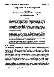
FIG. 1. Diagram of the projection of a TERMA voxel to the fluence plane. The forward method 共right兲 covers the voxel’s fluence area by casting a ray for each fluence pixel. Only the source blur is required. The back-projection method 共left兲 blurs the fluence area by the average projected voxel size. This is convolved with the source blur for efficiency.
architecture15 共CUDA兲 software development environment for GPU routines and the Digital Mars’ D programming language16 for CPU setup and analysis routines. II.A. Fluence generation
Incident fluence is typically generated by a model of the primary photon source, primary collimator, flattening filter, and various field modifiers available on a particular linear accelerator, such as collimator jaws, multileaf collimators 共MLCs兲, and wedges. In a deterministic dose calculation model, primary fluence is typically divided into spectral and intensity components. The spectral component has traditionally been parameterized by a single spectrum, an analytical off-axis softening function, and a discretized radial function of off-axis intensity factors. We have combined these components into a single, discretized radial spectral function, which contains a full spectrum at each off-axis angle. This provides more modeling flexibility, allowing the parameters to be determined by alternative analytical functions, Monte Carlo simulations, or direct optimization against measured data. We support wedges by combining the discretized radial spectral function with the wedge properties to generate a discretized Cartesian spectral function. The intensity component accounts for field modifiers, such as collimator jaws or MLCs. These are generally modeled using a simple transmission factor. We use a transmission factor for the jaws and precisely calculate the transmission though the MLC via the ray-path length and a linear attenuation constant. MLCs with round leaf ends are typically modeled with a symmetric, circular end, although this may not be physically true. We allow the circular end to be vertically offset, instead of symmetric, in order to better model the rounded leaf ends of certain vendors. Our current primary fluence implementation combines point sampling with anti-aliasing like over-sampling to produce accurate results. One modeling issue unique to our application comes from our back-projected TERMA computation. As seen in Fig. 1, each back-projection voxel must integrate the fluence area which contributes to them. For efficiency, we compute these contributors by adding a voxelsize blur to the generated fluence. In practice, we combine
296
Jacques et al.: Real-time dose computation: GPU-accelerated source modeling and superposition/convolution
the voxel-size blur with the source-size blur. A source-size blur is a standard method of modeling the physical size of the primary source. Both blurs are modeled using Gaussian functions and computed using separated 1D convolutions. Extra-focal 共scatter兲 sources are created in the linear accelerator treatment head by the interaction of the primary fluence with beam modifiers. The largest secondary source of radiation is the flattening filter, which contributes up to 15% of the dose to the patient.17 Other extra-focal sources are considered to be minor and result in slightly reduced model quality.18 We therefore have limited our current implementation to one extra-focal source, the flattening filter. Our model, never the less, is capable of multiple extra-focal sources. Unlike the primary source, which is point-like, extra-focal sources are area sources. However, to reduce computation, the extra-focal fluence to a reference plane is calculated and projected through the volume. This projection uses a second, virtual point source, which is closer to the isocenter than the primary target, and has a separate discretized radial spectral function.17 Extra-focal sources are further approximated as being isotropic area sources. Though not physically correct, the anisotropic components have mostly the same direction as the primary fluence. This allows the anisotropic portions of the flattening filter fluence to be incorporated in the primary source model. By using a second approximation, that only unobstructed source areas contribute fluence, the isotropic approximation allows the explicit calculation of the contribution of every pixel of source to every pixel of fluence to be avoided. Thus, the extra-focal intensity is calculated by integrating the source area viewable from each point on the reference plane. To make this calculation efficient, previous source models have used analytical functions and their analytical integrals to model the fluence. Unfortunately, the use of analytical integrals resulted in one further, problematic approximation: that the MLC leaves are infinitely thin. The viewable source area is defined as the projection of the MLCs and jaws back to the source plane. Figure 2 illustrates the reduction in viewable source area that occurs due to the heights of the MLC leaves. In highly modulated fields, such as in Fig. 3, this can substantially reduce extra-focal fluence. Even disregarding some of the subtler effects of rounded leaf ends or a particular manufacturer’s tongue-and-groove design, one is left with a complex outline for which it is nontrivial to find a set of integration rectangles that cover it. Instead of an analytical function, our extra-focal model utilizes an arbitrary, discretized function. This allows for multiple types of extra-focal sources to be modeled, for a better fit to measured or Monte Carlo data and for MLC leaf heights effects to be accounted for. We use a sum area table19 to provide an efficient integral calculation. A sum area table, sat, is a function which at every point, x, y, contains the integral of an image, I, from the origin corner to that point Medical Physics, Vol. 38, No. 1, January 2011
∞ Thin MLCs
296
Normal MLCs
FIG. 2. Diagrams depicting extra-focal source modeling with 共right兲 and without 共left兲 MLC leaf height effects. The yz-plane diagram 共top兲 shows the effects of closed 共black兲 leaves shadowing open 共white兲 MLCs. The xy-plane 共bottom兲 shows the difference in source integration patterns between summing each rectangle 共left兲 and alternatively adding and subtracting each vertex point of an arbitrary outline 共right兲. The black dot represents the calculation point on the reference plane through the isocenter.
x
y
sat共x,y兲 = 兺 兺 I共i, j兲.
共1兲
i=0 j=0
The image may be any discretized function e.g., the extrafocal source fluence. The sum area table can then be used to efficiently calculate the integral of any rectangle, defined by a set of upper, xu, y u and lower, xl, y l, bounds by sat共xu,y u,xl,y l兲 = sat共xu,y u兲 − sat共xu,y l兲 + sat共xl,y l兲 − sat共xl,y u兲.
共2兲
By extension, an arbitrary shape consisting only of straight lines and right angles, such as the viewable source area, can be integrated, as depicted in Fig. 2, by walking the shape’s boundary alternatively adding and subtracting at every corner. In our implementation, the viewable source area boundary is generated by breaking the area into two parts: the areas above and below the calculation point. The boundary of each can then be found by walking away from the calculation point, allowing MLC leaf height effects to be determined in a straightforward manner. We maintain numerical accuracy by limiting the size of the sum area table to under 256 ⫻ 256 pixels, by computing the lower viewable source area first, by using separate field and control point accumulators, and by pairing subtractions and additions. We found the effects of using double precision or Kahan summation20 to be
MLC field shape
∞ Thin MLCs
Normal MLCs
FIG. 3. Example field 共left兲 showing the effects of MLC leaf height on extra-focal fluence. Using infinitely thin MLCs 共center兲 increased extrafocal fluence by a factor of ⬃2 compared to MLCs with a normal height 共right兲.
297
Jacques et al.: Real-time dose computation: GPU-accelerated source modeling and superposition/convolution
negligible. In our previous work, we implemented a rudimentary jaws-only dual-source model. The differences between our previous, jaws-only extra-focal model and our new extra-focal model for several open fields were negligible. These results indicate that the truncation error of our viewable source integration is negligible. We define negligible in this situation to be under the 32-bit floating point machine epsilon; the smallest increment to the value 1. II.B. Fluence transport
The superposition/convolution21–23 algorithm consists of two stages. First, fluence is transported through the patient to compute the TERMA in the volume. Then superposition spreads the TERMA by a dose deposition kernel to determine the final dose at each location. To allow the dose deposition kernel to scale realistically with tissue inhomogeneities, the radiological distance, d p, Eq. 共3兲 between two points, r and s, is used. This weighting of distance by the electron density 共relative to water兲, , differentiates superposition from traditional convolution. d共r⬘,s兲 =
冕
s
r⬘
共t兲dt.
共3兲
II.B.1. TERMA The TERMA, TE共r⬘兲, of a particular photon energy E at point r⬘ is defined as the energy’s fluence, ⌿E, weighted by the density relative to water, , and the linear attenuation constant, E, at point r⬘ TE共r⬘兲 =
E共r⬘兲 ⌿E共r⬘兲. 共r⬘兲
共4兲
The energy’s fluence, ⌿E, to point r⬘ is determined by the incident fluence, ⌿E,0, from the source focal point, s, towards point r⬘ attenuated by the material between them and scaled by the distance squared effect ⌿E共r⬘兲 =
⌿E,0共r⬘兲 兰s − 共t兲dt e r⬘ E . 储r⬘ − s储2
共5兲
Traditionally, TERMA has been calculated by a forwardprojection of the fluence through the patient volume using an approximation of Eq. 共5兲 ⌿E共r⬘兲 =
⌿E,0共r⬘兲 −共 共r⬘兲/共r⬘兲兲⫻d 共r⬘,s兲 p e E . 储r⬘ − s储2
共6兲
Equation 共6兲 may be calculated from the radiological depth of a point, making it more computationally efficient. Equation 共6兲 also allows the exponential to be cached in a 3D lookup table. However, this lookup table exceeds the GPUcache size, resulting in poor performance. Instead, we use the GPU’s dedicated hardware exponential to calculate the attenuation. This allows the use of exact radiological path ray-tracing,24 which reduces artifacts and permits the use of the physically correct, multispectral attenuation from Eq. 共5兲. Our previous implementation of Eq. 共5兲 interpolated the linear attenuation for every energy at every voxel. Even with Medical Physics, Vol. 38, No. 1, January 2011
297
hardware acceleration, this created a major performance bottleneck. To address this issue, we utilized the sparsity of the set of materials, M, in the density normalized linear attenuation table to rearrange the attenuation integration from Eq. 共5兲 to
冕
s
r⬘
− E共t兲dt = − 兺 M
E,M M
冕
s
r⬘
␣M 共t兲共t兲dt.
共7兲
As the linear interpolation coefficient for a material, ␣ M , is common to all energies, Eq. 共7兲 allows the energetic specific attenuation properties to be moved outside the inner raytracing loop, enhancing both performance and accuracy. The traditional forward-projection method of calculating TERMA is fundamentally serial. To parallelize, we utilized the inherent ray divergence of projection to identify sets of rays which could be run in parallel. This strategy introduced extra GPU call overhead, fragmented the workload into smaller, less efficient work units, and introduced memory inefficiencies; the GPU loads memory in 128-bit words resulting in a memory efficiency of 25%–50%. This inefficiency is compounded by the fact no two rays in a set reference the same voxel, drastically reducing the cache efficiency of the density lookup. Furthermore, in order to ensure good fluence sampling, at least four rays must pass through each voxel. This necessitates an additional “ray-path length” volume in order to correctly average the fluence-ray TERMA contributions. To address these issues we developed a back-projected TERMA algorithm,6 which casts a ray from each TERMA voxel back towards the source, gathering the attenuation along the way. While this is an O共n4兲 algorithm, as opposed to the standard O共n⬃3兲 method, it eliminates certain discretization artifacts, it is fully parallel, and it exhibits a large degree of cache reuse; we found that doubling the number of threads per cache unit nearly doubled the performance. Theoretically, this performance gain continues so long as more than one element per thread can be stored in cache. We also enhanced the performance of the TERMA calculation when only changes in the fluence intensity occur, as is common during treatment plan optimization. This was achieved by formulating the TERMA calculation as an incident fluence, ⌿0, scaled by an attenuation factor, A, which can be mono-energetic or poly-energetic. As superposition normally uses the poly-energetic TERMA Eq. 共8兲, we use the poly-energetic attenuation Eq. 共9兲 to compute the polyenergetic TERMA using Eq. 共10兲. T共r⬘兲 = 兺 TE共r⬘兲,
共8兲
E
A共r⬘兲 =
1 E⌿ 共r⬘兲 E 兰r⬘− 共t兲dt es E , 兺 E,0 储r⬘ − s储2 E 兺EE⌿E,0共r⬘兲 共r⬘兲
T共r⬘兲 = ⌿0共r⬘兲A共r⬘兲.
共9兲
共10兲
298
Jacques et al.: Real-time dose computation: GPU-accelerated source modeling and superposition/convolution Ideal
II.B.2. Superposition Superposition spreads the TERMA by a dose deposition kernel,25,26 KE, to determine the final dose, D, at a location, r. KE is specific to an energy E and is indexed by the radiological distance Eq. 共3兲 and the relative angle, , between the point and the kernel axis, but lacks the geometric distance squared effect. We have chosen the standard inverse kernel method of superposition as it is both efficient and inherently parallel. D共r兲 =
∰兺
EW共r⬘兲TE共r⬘兲KE共d共r,r⬘兲, 共s,r,r⬘兲兲
E
⫻
1 dr⬘ . 储r − r⬘储2
共11兲
However, Eq. 共11兲 is not explicitly calculated. Instead, the mono-energetic kernels are simplified to a poly-energetic kernel using Eq. 共12兲, which is defined for a finite set of 共zenith兲 angles, a fixed number of azimuth angles per zenith angle, , and a energetically normalized spectrum. E⌿E,0 兺EE⌿E,0
K共dr, 兲 = 兺 E
冕
⌬w+
⌬w−
KE共dr, + w兲dw .
共12兲
This set of rays, v, negates the distance squared effect, as it is equal to the effect of the increase in volume of the solid angle the rays subtends and simplifies Eq. 共11兲 to Eq. 共13兲 D共r兲 ⬇ 兺
冕
T共r + t兲K共d共r,r + t兲, 共v兲兲dt.
共13兲
Kernel tilting27 occurs when the ray directions are relative to the source-to-r axis. A clinically acceptable approximation is to use ray directions that are relative to the beam axis, instead of the source-to-r axis. This introduces a small error in each direction’s zenith angle, , and therefore reduces accuracy. Directly using the dose deposition kernel is numerically unstable at clinical resolutions.28 Instead, either the CK,13 which represents the dose from a ray segment to a point, or the cumulative-cumulative kernel 共CCK兲,28 which represents the dose from a ray segment to a ray segment, are used. CK共x, 兲 =
冕
x
K共t, 兲dt,
共14兲
0
冕
x+⌬x
K共v, 兲dv = CK共x + ⌬x, 兲 − CK共x, 兲,
共15兲
x
CCK共x, 兲 =
冕
x
CK共t, 兲dt,
共16兲
0
冕冕 ⌬s
0
x+v+⌬x
K共u, 兲dudv
x+v
= 共CCK共x + ⌬s + ⌬x, 兲 − CCK共x + ⌬x, 兲兲 − 共CCK共x + ⌬s, 兲 − CCK共x, 兲兲. Medical Physics, Vol. 38, No. 1, January 2011
共17兲
Standard
50% Azimuth Phase
Multi-resolution
298 Truncated
FIG. 4. Diagrams of the memory access patterns of the different superposition methods 共top兲 with example dose depositions from a 5 mm field 共bottom兲. From left to right: ideal, standard, standard with a 50% azimuth phase offset, multi-resolution, and truncated. Identical windows and levels were used. Note the standard’s star pattern, the “extra” azimuth rays due to changing the azimuth angle phase, the multi-resolution’s gridding artifacts, and the truncation distance.
We experimented with both the CK and the CCK and chose to use the CCK as it provides greater accuracy, particularly at coarser resolutions, at little computational cost. The ability to use a coarser resolution is important; a two times reduction in resolution results in a ⬃16 times increase in performance. We implemented both kernel tilting and kernel non-tilting superposition algorithms. Kernel tilting is slightly more complex and has poorer cache performance than kernel nontilting. However, kernel tilting provides greater accuracy which allows the number of kernel rays to be reduced, resulting in a net gain in effective performance. In addition to this cost, using kernel tilting prevents ray-trace index caching, one of the major optimizations found in Pinnacle3. Due to the computational performance and limited cache sizes on the GPU, we chose not to use this optimization in our nontilted kernels. II.B.3. Multi-resolution superposition The ability of the CCK to remain accurate at coarse resolutions allowed us to develop a multi-resolution superposition algorithm, which approximated each sample ray as a true solid angle. As a ray’s width is proportional to the voxel width, by increasing the voxel size with geometric distance, the growth of the associated solid angle can be approximately matched. This improves theoretical complexity from O共N4兲 to O共N3 log N兲 for a cube water phantom of side length N. Multi-resolution superposition reduces small field 共star兲 artifacts 共see Fig. 4兲 which occur when an entire beam is missed due to sparse azimuth ray sampling. However, larger step sizes decrease the dose deposition kernel accuracy as the beam’s boundary is blurred, resulting in a systematic underdosage. Additional artifacts are introduced when neighboring voxels transverse different coarse resolution voxels. Our implementation uses volumetric mip-maps;29 a set of images generated by sampling the input image at different resolutions. We set the resolution of each mip-map “level” to be half the resolution of the preceding level. This makes multi-resolution superposition inherently isotropic. Mip-map resolution changes were limited to a maximum of once per step and were only allowed to occur at voxel boundaries in
299
Jacques et al.: Real-time dose computation: GPU-accelerated source modeling and superposition/convolution
the coarser resolution in order to prevent a TERMA voxel from contributing multiple times to the same dose voxel. II.B.4. Arc superposition An unintuitive facet of non-tilted kernels is that they contain up to ⬃5° of superposition angular error, depending on field size. This has been shown to be clinically acceptable when the TERMA is correct. Applying this proven approximation to arc therapy leads to the novel enhancement of using different angular sampling for the TERMA and superposition computations. As TERMA calculations are substantially faster than superposition calculations, using a high TERMA and a low superposition angular resolution can dramatically increase the performance and accuracy of arc therapy calculations. II.B.5. Delta superposition Currently, superposition is not fully used for inverse planning optimization due to low performance and the lack of a derivative algorithm. Though our GPU method is fast, optimizers can utilize a delta dose computation: the ability to reduce the workload by only adding the change, or delta, in primary fluence to the current dose deposition. There are three ways to extend delta dose computation to our method. First, we employ an early ray termination optimization. This sentinel can be utilized to artificially truncate the calculation to a radius about the primary fluence in a manner similar to pencil beam. The elegance of this solution is that it uses the same code base as normal superposition. So when all fluence points change, full superposition accuracy is obtained. However, adding and subtracting a beamlet can introduce errors as each change may be computed with a different accuracy. Next, the consistency of the first method can be increased by setting a fixed truncation distance, perpendicular from the beam’s axis. We found the relative performance of truncated superposition to decrease with finer resolutions: It was relatively fastest at 4 mm3, but at 1.9 mm3 its performance was worse than that of multi-resolution superposition. Lastly, full dose deposition can be calculated for the subset of voxels that would normally be affected by a delta dose computation. The subset may be flagged using a sentinel dose value, eliminating the extra storage and memory bandwidth required by a separate mask volume. Recalculation is more accurate and can include the changes in extra-focal fluence. This should increase the time between or eliminate the need for the periodic full superposition recalculations traditionally required by delta dose computations. II.C. Optimizing
CUDA
performance
Several strategies were used to optimize CUDA performance. CUDA’s execution model is a 2D grid of 3D blocks of threads which execute a function 共called a kernel兲. Each block represents one parallel work unit and therefore is limited in size. Block thread counts were optimized using NVIDIA’s CUDA occupancy calculator, maximizing for both occupancy and total block size. We refactored our tilted kerMedical Physics, Vol. 38, No. 1, January 2011
299
nel implementation to allow for the maximum block size 共512 threads兲 to be used. This added one additional texture lookup per ray, but increased cache sharing. The rearrangement of the multispectral TERMA equation to Eq. 共7兲 increased the TERMA block size from 192 to 512 threads. The only functions where we did not achieve the maximum block size were the extra-focal source, the truncated superposition, and the multi-resolution superposition routines. These all used blocks with 384 threads. For volume processing, we used a 1:1 mapping of threads to voxels in the x and y directions. The z direction was handled by looping over the per voxel function with increasing z indices. We used cube-like block dimensions and a z stride of the z block size to maintain thread spatial cohesion. This reduced cache misses and increased performance. All input array data was cached, generally in textures, which, in the case of superposition, doubled performance. The exception to this was the attenuation material properties, which were cached in constant memory. Thread block synchronization was used to further maintain superposition thread spatial cohesion. This had a negligible performance impact at low resolutions, but increased high resolution performance by up to 21%. Non-tilted superposition used a single synchronization at the start of each kernel ray. Tilted superposition used two synchronizations: one at the start of each kernel ray and one at the start of each ray-trace. TERMA and multi-resolution superposition did not benefit from explicit synchronization. We further reduced global memory bandwidth over our previous implementation by using a joint structure of two 16-bit floating point numbers for transferring the TERMA and density, , volumes to the superposition algorithm. This resulted in a performance gain of ⬃13% and an average truncation error of 1.8⫻ 10−5% of Dmax, which is under the 16-bit floating point machine epsilon. The lower than expected performance gain of 16-bit floats indicates a shift in the performance bottleneck away from global memory bandwidth. 16-bit floats were not used for the TERMA calculation; passing the attenuation volume with 16-bit floats had a negligible performance benefit and resulted in additional truncation error, while passing the density volume with 16bit floats actually reduced performance due to the extra workload of unpacking the 16-bit floats inside the ray-tracing loop. Shared memory is a small, fast memory area shared between all threads in an execution block. Shared memory was used to store each control point’s MLC leaves in the extrafocal fluence computation and the array of volumes defining the mip-mapped data structure used in multi-resolution superposition. Previously, we used shared memory to store the multispectral attenuation bins in the TERMA computation, as it offered a slight performance improvement over registers, which spilled the attenuation bins into local memory; we allowed a maximum number of 21 energy bins as it was both sufficient for high energy beams and was free of shared memory bank conflicts, which can reduce performance. The improved TERMA implementation instead requires an accumulator for each material and supports up to 12 materials at
300
Jacques et al.: Real-time dose computation: GPU-accelerated source modeling and superposition/convolution
the maximum block size. Our attenuation tables contained nine materials: registers were used for the four common, biological materials and shared memory for the five less common metals. Using shared memory to store the MLC leaves for each primary fluence control point had worse performance than using the texture cache, as not all leaves were used by each execution block. II.D. Analysis methodology
Quantitative analysis of a transport algorithm, such as superposition/convolution, is complicated by a strong dependence on the incidence fluence from the source model.30,31 The source model in turn is optimized to minimize the error between measured dose and calculated dose. Thus, the source model often masks errors in the transport algorithm. We have yet to complete a commissioning process for our source model, preventing us from fully leveraging its capabilities. Furthermore, commercial systems also included a separate electron contamination model, which is not considered in our implementation. We based our system parameters on a commissioned Varian 6EX linear accelerator modeled in the Pinnacle3 treatment planning system, with the exception of the beam spectrum where we used the published reference spectrum. The MLC contained 40 1 cm wide leaves with rounded leaf ends. The spectrum contained 15 spectral bins. Mass attenuation tables and mono-energetic dose deposition kernels were provided by Pinnacle3. CT to density conversion was achieved using a standard piecewise-linear function. II.D.1. Performance metrics All performance results are reported as raw numbers and the absolute speedup where appropriate, as this is the preferred method in parallelization research. Most of the publications related to this work have reported performance in relative speedup. The difference between relative and absolute speedup is that the former is relative to a version of the algorithm, while absolute speedup is relative to the optimal version of the algorithm. This can be a substantial factor as, for example, based on Hissoiny et al., Pinnacle3 is at least 2.3 times faster than PlanUNC. In this paper we only report absolute speedup, using Pinnacle3 共Philips, Madison, WI兲 as our optimal serial reference, as we are unaware of any serial implementation with better performance. Although Pinnacle3’s adaptive superposition is technically the fastest clinically acceptable superposition/convolution algorithm, it is next to impossible to get two implementations of adaptive superposition to perform the same workload, and thus quantitative comparisons are not possible. We have refrained from making quantitative speedup comparisons between methods where the quantitative accuracy of the slower method is higher. II.D.2. Performance measurements Source model tests used a fluence size of 4002 pixels at a 1 mm2 resolution. Superposition tests were performed on a Medical Physics, Vol. 38, No. 1, January 2011
300
cube water phantom with a side length of 25.6 cm. Tests were performed on a dose volume with 643 voxels, which is representative of standard clinical workload and an additional high resolution volume with 1283 voxels. Both volumes were centered at the beam isocenter. All Pinnacle3 experiments were run on an AMD 共Sunnyvale, CA兲 Opteron 254 共two cores, 2.8GHz兲. Timing experiments were repeated at least ten times with no other programs active, using the standard superposition/convolution engine, with full heterogeneity correction. Time was measured by hand from the start of the superposition computation to the end, as reported by the Pinnacle3 user interface. The performance of Pinnacle3’s setup, fluence generation, and TERMA computations were not measured. GPU experiments were performed on a Core i7 920 共four cores, 2.67GHz兲 with a single NVIDIA GeForce GTX 280 GPU. Timing results were repeated multiple times using the high performance hardware counter of the CPU 共with execution limited to a single core to prevent errors兲 and include all steps required to execute that phase of computation. For example, the multi-resolution superposition times include the volumetric mip-map generation. For clarity, like Pinnacle3, we consider the loading and setup of the beam definition a separate step. This step is of similar complexity on both the CPU and GPU. However, the GPU can accelerate certain tasks, such as the conversion and resampling of the CT data set to density, and hide the cost of others by concurrently running different CPU and GPU tasks. Further, we assume comprehensive GPU use. Specifically, that algorithm inputs are generated on the GPU whenever possible and that the final dose output is summed, visualized, analyzed, etc., primarily using GPU routines. When this is not the case, it is possible for the GPU to write directly to main memory and for the next GPU generation to read directly from main memory, avoiding unnecessary memory copies. II.D.3. Kernel ray sampling The selection of the kernel ray directions for superposition is one of the black arts of dose computation. The set of rays has to balance the sampling of the patient representation, the incident fluence and the kernel itself. Traditionally, the kernel is sampled using a set of equally spaced azimuth angles and variably spaced zenith angles. The zenith and azimuth sampling directly affect the kernel and incident fluence sampling, respectively, and their combined properties effect the sampling of the patient representation. As zenith angles range from 0° to 180° while azimuth angles range from 0° to 360°, it takes twice as many azimuth angles as zenith angles to achieve the same angular sampling. Pinnacle3 uses ten zenith and eight azimuth angles normally and has a “fast” mode which only uses four zenith angles. Pinnacle3’s sampling of the ten zenith angles is a trade secret, but is known to be neither isotropic nor isoenergetic and was designed to counteract the accuracy lost from not tilting the kernel. We have created multiple sampling routines which attempt to create a set of isoenergetic zenith bins given a maximum zenith angle constraint. Each
301
Jacques et al.: Real-time dose computation: GPU-accelerated source modeling and superposition/convolution
routine binned the mono-kernel zenith angles in a greedy fashion, starting with the most backwards angle and proceeding toward the most forwards angle. They differed in how they handled the maximum zenith angle constraint: one always slightly exceeded the constraint, one met or exceeded the constraint, and one “looked ahead” to determine whether to exceed, meet, or fall short of the constraint. This allowed us to experiment with a variety of ray samplings from fully isotropic to fully isoenergetic. We experimented with increasing the phase of the azimuth sampling with each zenith bin 共see Fig. 4兲, with adding a single ray along the beam axis in both the forwards and backwards directions, and with both geometric and energetic weightings for each zenith bin ray.
301
TABLE I. Performance of multiple TERMA calculation methods on an NVIDIA GeForce GTX 280. The prior forward and prior backward methods used multispectral attenuation and have been previously reported 共Ref. 7兲. Multispectral and homogeneous methods both use back-projection. The cached method is projection method agnostic. Volume size Method
643
1283
2563
Prior forward, Eq. 共5兲 Prior backward, Eq. 共5兲 Multispectral, Eq. 共7兲 Homogeneous, Eq. 共6兲 Cached, Eq. 共9兲
44 ms 18 ms 3.5ms 1.7ms 0.2ms
150 ms 220 ms 34.5ms 27.0ms 1.2ms
1869 ms 3371 ms 438.0ms 362.8ms 9.8ms
II.D.4. Accuracy measurements At this point a final commissioned model is not available, so we measure the algorithmic accuracy of practical superposition implementations against an ideal superposition computation. Our ideal superposition computation is made using the tilted inverse cumulative-cumulative kernel sampled using the native 48 zenith angles of the monokernel data and 96 azimuth angles. Several delivery setups were tested including an IMRT treatment. In order to report our results we have chosen to average the mean error, relative to the maximum dose of the reference calculation, across a set of test fields. This is an improvement over our previous work, as it incorporates the systematic, absolute dose shifts that occur with multi-resolution, and truncated superposition. We used two test field sets: a set of 47 square fields ranging from 0.5 cm⫻ 0.5 cm to 23 cm⫻ 23 cm in 0.5 cm increments and a set of 18 IMRT fields from a head-and-neck cancer patient 共nine primary and nine cone-down兲. The field sets were delivered to a water phantom and the IMRT patient data set. Less extensive experiments using the synthetic field sets delivered to a heterogeneous slab phantom and additional patient data sets were performed.
algorithms for a range of resolutions. All three algorithms incorporated the physically correct multispectral attenuation from Eq. 共5兲. The back-projection algorithm exhibited an empirical complexity of O共n⬃3.5兲 which is a slight improvement over its theoretical complexity of O共n4兲. We also implemented the homogenous material attenuation approximation from Eq. 共6兲. This approximation increased performance by 24%. We found that caching the attenuation value provided a substantial performance increase; however, it may only be used when changes are limited to the incident fluence. We have previously shown our back-projection TERMA formulation to have very good agreement with an analytical formulation and to be within the discretization artifacts of Pinnacle3’s forward-projection implementation.7 Comparisons between our new and old multispectral implementations of Eq. 共5兲, with the homogeneous approximation Eq. 共6兲, showed Eq. 共7兲 eliminated truncation errors and had perfect agreement for certain homogeneous slabs. Comparisons between the two implementations using heterogeneous volumes showed good agreement with no systematic trends; the maximum error was within the floating point epsilon.
III. RESULTS
III.B.2. Superposition
III.A. Fluence generation
Table II compares the performance for a variety of superposition methods. We used the more accurate CCK 关Eq. 共16兲兴 instead of the traditional CK 关Eq. 共14兲兴 for all reported results. We found the CCK was between 0.7% 共1283 voxels兲 and 4.8% 共643 voxels兲 slower than the CK, depending primarily on volume resolution but also superposition method and GPU architecture. Comparatively, CPU implementations of the CCK are 50% slower than the CK.28 We found kernel tilting on the GPU to have an average performance cost of 10% for standard superposition and 4% for multi-resolution superposition. This indicates that the majority of performance loss is due to ray divergence, which occurs during tilting, resulting in poorer memory performance. Comparatively, CPU implementations of kernel tilting have resulted in a 300% performance loss.27 As can be seen in Table II, kernel tilting offers a substantial accuracy increase, particularly in the gradient region. This increased accuracy can be used to reduce the number of kernel sampling rays resulting in a net performance gain of ⬃56%.
The performance of the primary source model was 0.15 ms for a single control point. The performance of the extrafocal source was under 5.3 ms for a single control point and was both MLC and jaw position dependent. The jaws perpendicular to the MLCs had the largest effect, as they limited the number of leaves that needed to be fully processed. MLC data was observed to affect performance by up to 50%. Total time, including source blurring, was under 8.3 ms. Tests performed using a fluence size of 8002 pixels indicates an empirical complexity of O共n1.8兲 which is slightly better than the theoretical O共n2兲. III.B. Fluence transport
III.B.1. TERMA In Table I we compare the performance of our improved back-projected TERMA algorithm to our previous GPU versions of the forward-projection and back-projection TERMA Medical Physics, Vol. 38, No. 1, January 2011
302
Jacques et al.: Real-time dose computation: GPU-accelerated source modeling and superposition/convolution
TABLE II. Comparison of superposition performance on cube water phantoms. Full heterogeneity correction was used. Using tilting with 4 ⫻ 8 or 6 ⫻ 12 rays had greater accuracy than using 10⫻ 8 rays without tilting 共see Table III兲. Timing experiments were repeated at least ten times on a Core i7 920 共four cores, 2.67GHz兲 with an NVIDIA GeForce GTX 280 共GPU兲 and AMD Opteron 254 共two cores, 2.8GHz兲 共Pinnacle3, Philips, Madison, WI兲. The Pinnacle3 times were hand measured, with standard deviations of 84 and 544 ms for the 643 and 1283 volumes, respectively. GPU times were measured using the CPU’s high performance counter with execution limited to a single core.
Method Standard Standard Standard Standard Multi-Resolution Multi-Resolution Truncated Pinnacle3
Type Tilt Rays CCK 10x8 CCK 6x12 CCK 10x8 CCK 4x8 CCK 4x8 CCK 4x8 CCK 4x8 CK 10x8
643 1283 Time(s) Speedup Time (s) Speedup 0.146 57x 2.276 42x 0.129 64x 2.097 45x 0.124 66x 2.026 47x 0.058 144x 0.936 101x 0.058 N/A 0.422 N/A 0.053 N/A 0.392 N/A 0.031 N/A 0.385 N/A 8.268 1x 94.508 1x
302
thetic square field set had greater error than patient data sets, most likely due to increased long-distance patient scatter dose. Superposition method was the most influential factor on accuracy; from best to worse were: tilted, non-tilted, tilted multi-resolution, multi-resolution, and truncated. There were several exceptions to this generalization. The 4 ⫻ 8 tilted kernels had similar 共and therefore sometimes worse兲 performance to the best non-tilted kernels in the high dose region, but were better in the gradient and low dose regions. The truncated kernels performed better with the IMRT fields and patient data sets, sometimes outperforming the multiresolution kernels. However, this only occurred with anisotropic kernels, which reduces the performance benefits of truncation and are inherently a poor choice for multiresolution superposition. Multi-resolution superposition performed best with isotropic kernels, as was expected. Changing the ray sampling method and/or adding axis-aligned rays generally provided marginal mixed results. The exception to this was the 4 ⫻ 8 kernel samplings with a backwards axisaligned ray. Adding an azimuth phase offset to each zenith bin generally provided a marginal improvement in accuracy, though a worsening of accuracy did occur for some experiments. The notable exceptions to this were the 10⫻ 8 kernel samplings with the tilted and, to a lesser degree, the non-tilted methods.
Empirical O(n) O(n3.96) O(n4.02) O(n4.02) O(n4.02) O(n2.86) O(n2.89) O(n3.61) O(n3.51)
In Table III we compare the accuracy of a selected set of superposition methods and samplings. The set includes interesting, clinically relevant results from a simulated head-andneck IMRT delivery. Our full set of experiments included two field sets, seven phases, 101 kernel samplings, and multiple test volumes. Generally, all experiments were qualitatively similar. Quantitatively, cube phantoms and the syn-
TABLE III. Selected average mean deposited dose errors, relative to Dmax, for 18 IMRT fields 共nine primary and nine cone-down兲 from a head-and-neck cancer patient, delivered to the patient’s volume for multiple superposition methods and kernel ray samplings. The ray sampling are defined by the number of zenith angles and by the number of azimuth angles, and may include a azimuth phase offset 共⌬兲, energetic angle weightings 共WE兲, a forward ray 共F兲, and/or a backward ray 共B兲. The WE kernels used a ray sampler with look-ahead. Reference dose deposition was calculated using a tilted kernel sampled with 48 ⫻ 96 rays. An absolute dosimetry error of 2%–5% is clinically acceptable 共Ref. 3兲.
No. of Rays Notes: Zenith Angle Max
π
π/4
Tilted Not-tilted Tilted-multi-res. M ulti-resolution Truncated
0.14% 0.25% 0.88% 0.98% 1.16%
0.13% 0.24% 0.87% 0.97% 1.16%
0.07% 0.22% 0.88% 0.98% 1.16%
0.07% 0.22% 0.88% 0.99% 1.16%
0.13% 0.23% 0.87% 0.97% 1.15%
High Dose Region 0.16% 0.12% 0.18% 0.30% 0.24% 0.28% 0.69% 0.61% 0.73% 0.79% 0.73% 0.83% 1.21% 1.12% 1.13%
Tilted Not-tilted Tilted-multi-res. M ulti-resolution Truncated
0.20% 0.55% 0.83% 1.08% 1.01%
0.18% 0.52% 0.81% 1.05% 1.01%
0.11% 0.52% 0.80% 1.06% 1.00%
0.11% 0.51% 0.80% 1.06% 1.01%
0.18% 0.53% 0.81% 1.06% 1.00%
Tilted Not-tilted Tilted-multi-res. M ulti-resolution Truncated
0.09% 0.16% 0.13% 0.19% 0.42%
0.09% 0.13% 0.11% 0.17% 0.42%
0.05% 0.12% 0.11% 0.16% 0.42%
0.05% 0.12% 0.11% 0.16% 0.42%
0.08% 0.13% 0.11% 0.16% 0.42%
10×8 0.5 ∆φ 0.6 ∆φ π/4 π/4
Medical Physics, Vol. 38, No. 1, January 2011
π/4
WE π/4
4×8+F WE π/4
0.25% 0.34% 0.87% 0.98% 1.24%
0.28% 0.36% 0.84% 0.95% 1.31%
0.22% 0.32% 0.94% 1.03% 1.29%
0.19% 0.29% 0.86% 0.97% 1.20%
0.17% 0.27% 0.95% 1.05% 1.20%
Gradient Region 0.25% 0.18% 0.60% 0.54% 0.64% 0.55% 0.93% 0.86% 1.07% 0.97%
(|∇ D |> 0.3D ) 0.27% 0.35% 0.55% 0.59% 0.67% 0.84% 0.93% 1.09% 1.02% 1.13%
0.37% 0.66% 0.83% 1.11% 1.20%
0.33% 0.64% 0.95% 1.18% 1.17%
0.27% 0.56% 0.82% 1.09% 1.06%
0.26% 0.57% 0.94% 1.17% 1.06%
Low Dose Region 0.10% 0.06% 0.18% 0.12% 0.13% 0.09% 0.20% 0.15% 0.42% 0.41%
(D < 0.1D max ) 0.09% 0.12% 0.13% 0.15% 0.11% 0.13% 0.16% 0.18% 0.41% 0.42%
0.12% 0.15% 0.13% 0.18% 0.42%
0.12% 0.14% 0.13% 0.18% 0.43%
0.11% 0.14% 0.12% 0.17% 0.41%
0.11% 0.14% 0.13% 0.17% 0.42%
6×12 π/8
π
π/6
5×10 π/5
4×8
4×8+B WE π/4
4×8+FB WE π/4
303
Jacques et al.: Real-time dose computation: GPU-accelerated source modeling and superposition/convolution Water Tank
120
70
Pinnacle3
Tank Y 10cm
60
GPU
Pinn Y 10cm
50
80
Relative Dose
Relative Dose
100
303
60 40
GPU Y 10cm
40 30 20
20
10 0
0 0
5
10
15 Depth (cm)
20
25
30
-10
-9
-8
-7
-6
-5
-4
-3
-2
-1 0 1 Distance (cm)
2
3
4
5
6
7
8
9
10
FIG. 5. The central axis dose depositions from measured water tank data and the Pinnacle3 and GPU superposition implementations for a 10 cm field; normalized at a depth of 10 cm.
FIG. 6. The y-axis dose deposition profiles from measured water tank data and the Pinnacle3 and GPU superposition implementations at a depth of 10 cm; normalized at the midpoint.
The greatest improvements were seen with phases that were roughly one half the azimuth angle sampling. Experiments indicated the accuracy of a 10⫻ 8 kernel with 50% phase was similar to that of a 10⫻ 12 kernel without phase; an increase of 50%. This increase in effective azimuth sampling was supported visually by a reduction in star field artifacts 共see Fig. 4兲. Figures 5 and 6 compare the central axis and 10 cm dose profiles of the GPU implementation to Pinnacle3 and measured water tank data. Our implementation shows good agreement with some notable discrepancies. The minor central axis difference is indicative of a slightly harder beam spectrum. This effect may be due to slight differences in the spectrum, in spectrum interpolation, or in the dosedeposition kernel zenith angle interpolation. This can be corrected with a minor change to the modeled beam spectra.
where the maximum amount of error occurs. For standard superposition, we added the angle error to the field’s gantry angle and compared it to a reference dose deposition, computed at the field’s gantry angle. For arc superposition, we computed the TERMA volume at the field’s gantry angle and the superposition dose deposition at the field’s gantry angle plus the angle error. Results are reported as the average error of multiple IMRT fields for various kernel ray and angular samplings. Though preliminary, these experiments indicate a reasonable accuracy can be achieved with as little as nine superposition calculations, which represents an orders of magnitude performance improvement for arc therapies, such as VMAT.
III.B.3. Multi-resolution superposition Multi-resolution superposition performed up to two times faster than traditional superposition. Performance gains were primarily due to better scalability; the multi-resolution method had an empirical performance of O共n2.9兲 compared to traditional superposition’s O共n4.0兲. Table III includes a comparison of the accuracy of multi-resolution superposition to traditional superposition. Individual analysis of the set of square fields indicated multi-resolution superposition performed better in the gradient and low dose regions of small fields due to less TERMA being geometrically missed by rays. This was at the expense of accuracy in the high dose region as the larger step sizes caused the beam boundary to be blurred. This blurring results in a systematic under-dosage when using multi-resolution superposition. A variant of the multi-resolution method, using the same step sizes, but not using a multi-resolution data structure increased error by ⬃60% and resulted in poor cache usage, reducing performance by ⬃50%. III.B.4. Arc superposition Table IV contains the results of our preliminary experiments in arc superposition for the high dose and gradient regions for the IMRT data set. We investigated the error in dose deposition halfway between two calculation points, Medical Physics, Vol. 38, No. 1, January 2011
III.C. System performance
Total system performance is dependent on several factors, including the beam geometry, the patient geometry, and the dose grid’s size, resolution, and location. We measured the performance of Pinnacle3 and our GPU system using as comparable settings as possible for a typical IMRT prostate case 共nine fields, 198 control points兲. The Pinnacle3 computation time was 87.6 s on average, while the GPU time was 1.0 s. Component wise, 5% of the GPU time was spent generating the incident fluence, 18% computing the TERMA, and 75% performing superposition. Less than 2% of the time was spent in an unoptimized CPU routine converting the control points into a set of apertures and transferring them to the GPU. This breakdown highlights a shift in the relative performance of the GPU TERMA and superposition algorithms as compared to their serial counterparts. IV. DISCUSSION We have implemented a GPU-accelerated dose engine with near real-time performance based on the superposition/ convolution algorithm. We have developed a modern, deterministic GPU-accelerated source model. The extra-focal fluence model was enhanced with arbitrary fluence profiles and MLC leaf height modeling. The TERMA calculation was enhanced with physically correct multispectral attenuation and back-projection, which is inherently parallel and eliminates ray discretization artifacts. Furthermore, the TERMA attenuation caching strategy improves performance for interactive
304
Jacques et al.: Real-time dose computation: GPU-accelerated source modeling and superposition/convolution
304
TABLE IV. Selected average mean deposited dose errors, relative to Dmax, for 18 IMRT fields 共nine primary and nine cone-down兲 from a head-and-neck cancer patient, delivered to a cube water phantom 共25.6 cm with 4 mm cube voxels兲 for multiple superposition methods, kernel samplings, and 360° arc sampling schemes. Zenith angular sampling was limited by 2 / no. of azimuth angles.
Arc Superposition
Standard Superposition
Ra ys
6×12
4×8
4×8
4×8
10×8
6×12
4×8
4×8
4×8
Ti l t
Mul ti -res ol uti on No. of ∠'s ∞ 360 180 36 18 9
∆∠ 0° 0.5° 1° 5° 10° 20°
0.12% 0.12% 0.12% 0.27% 0.50% 1.07%
0.28% 0.28% 0.28% 0.31% 0.44% 0.92%
0.99% 0.99% 0.99% 1.02% 1.12% 1.48%
1.12% 1.12% 1.12% 1.16% 1.25% 1.60%
High Dose Region 0.27% 0.12% 0.32% 0.18% 0.40% 0.29% 2.73% 2.66% 7.05% 6.95% 14.05% 13.90%
0.28% 0.32% 0.40% 2.69% 6.96% 13.88%
0.99% 1.01% 1.05% 3.07% 7.21% 14.07%
1.12% 1.14% 1.18% 3.18% 7.30% 14.19%
∞ 360 180 36 18 9
0° 0.5° 1° 5° 10° 20°
0.14% 0.16% 0.18% 0.63% 1.24% 2.31%
0.31% 0.31% 0.32% 0.61% 1.08% 2.25%
0.88% 0.88% 0.89% 1.07% 1.42% 2.30%
Gradient Region (|∇ D |> 0.3D ) 1.12% 0.47% 0.14% 1.14% 1.30% 1.07% 1.14% 2.16% 1.99% 1.25% 7.63% 7.54% 1.52% 11.86% 11.77% 2.33% 17.08% 16.98%
0.31% 1.17% 2.05% 7.53% 11.74% 16.91%
0.88% 1.62% 2.40% 7.59% 11.75% 16.92%
1.12% 1.81% 2.56% 7.69% 11.83% 17.01%
use and intensity modulation optimization. We found several improvements to the superposition algorithm to be substantially more efficient on the GPU than on the CPU, warranting the main stream use of kernel tilting, the cumulativecumulative kernel, and exact radiological path ray-tracing. We explored the use of volumetric mip-maps to approximate solid angle ray-tracing during superposition dose deposition. Separating the angular sampling of the TERMA and superposition computations was found to increase the performance and accuracy of dynamic arc therapies.
transfer functions to implicit calculation is required. There is also an elegance in using superposition, and therefore the same source model, for both dose calculation and optimization. Superposition/convolution without transfer functions has not previously been used for inverse planning.
V.A.1. Derivative calculation using superposition/ convolution
V. FUTURE WORK A commissioning method for our source model, an electron contamination model, and a backscatter model are currently being completed. These will allow for a more quantitative assessment of the dose engine accuracy. We are investigating the use of analytical integration in the primary fluence model in order to better support therapies with dynamic MLCs such as VMAT. Though simple in the perpendicular direction, the rounded leaf end model would require simplification. Recent 3D texturing support may allow efficient approximate hardening of the dose deposition kernel. The recent switch to multiple instruction stream, multiple data stream style GPU architectures should allow for efficient implementation of adaptive superposition to the GPU. V.A. Inverse planning
Inverse planning systems currently utilize a combination of truncated transfer functions and either superposition or Monte Carlo dose calculation. In order to accelerate inverse planning on the GPU, a switch from using RAM intensive Medical Physics, Vol. 38, No. 1, January 2011
Most optimization methods utilize the derivative of the objective function in some manner. Even stochastic techniques, such as adaptive simulated annealing,32 which do not explicitly use the derivative in the optimization itself, use the derivative to set optimization parameters. The derivative of an objective function, O, with respect to the solution parameters, P, can be determined from propagating the object derivative with respect to dose, dO / dD, through superposition and the source model to the solution parameters. First, dD / dT is determined by reversing the forward superposition method; instead of spreading dose, the weighted effects of a unit of energy release are gathered. This is identical to using the inverse superposition method with a forward superposition kernel. dT / d⌿0 is then determined by a ray-cast algorithm, similar to the forward TERMA calculation, performing a similar gather weighted by each voxel’s attenuation. The source model then projects dT / d⌿0 to the machine parameters. Calculating d⌿0 / dP for extra focal sources algebraically is complex and most clinical systems approximate d⌿0 / dP as only being influenced by the primary source.
305
Jacques et al.: Real-time dose computation: GPU-accelerated source modeling and superposition/convolution
冉
冊
dO d⌿0 dT dD dO = . dP dP d⌿0 dT dD
共18兲
By integrating GPU-based dose and derivative computation, full utilization of our methods by future treatment planning systems will be possible. ACKNOWLEDGMENTS This work was funded in part by the National Science Foundation under Grant No. EEC9731748 and in part by Johns Hopkins University internal funds. Special thanks to Sami Hissoiny for discussions on and providing the results of their related work. a兲
Electronic mail:
[email protected] K. Otto, “Volumetric modulated arc therapy: IMRT in a single gantry arc,” Med. Phys. 35, 310–317 共2008兲. 2 D. Yan, F. Vicini, J. Wong, and A. Martinez, “Adaptive radiation therapy,” Phys. Med. Biol. 42, 123–132 共1997兲. 3 A. Ahnesjo and M. Aspradakis, “Dose calculations for external photon beams in radiotherapy,” Phys. Med. Biol. 44, R99–R155 共1999兲. 4 J. Krüger and R. Westermann, “Acceleration techniques for GPU-based volume rendering,” in Proceedings of the 14th IEEE Visualization Conference 共VIS ’03兲, 2003. 5 R. A. Jacques, R. H. Taylor, J. Wong, and T. R. McNutt, “SU-GG-T-511: Towards real-time radiation therapy: Superposition/convolution at 4fps,” Med. Phys. 35, 2842 共2008兲. 6 R. Jacques, R. Taylor, J. Wong, and T. McNutt, “Towards real-time radiation therapy: GPU accelerated superposition/convolution,” in Proceedings of the High-Performance MICCAI Workshop, 2008. 7 R. Jacques, R. Taylor, J. Wong, and T. McNutt, “Towards real-time radiation therapy: GPU accelerated superposition/convolution,” Comput. Methods Programs Biomed. 98共3兲, 285–292共2009兲. 8 M. de Greef, J. Crezee, J. C. van Eijk, R. Pool, and A. Bel, “Accelerated ray tracing for radiotherapy dose calculations on a GPU,” Med. Phys. 36, 4095–4102 共2009兲. 9 J. Gariépy, S. Hissoiny, J. Carrier, B. Ozell, and P. Després, “SU-FF-T622: Fast GPU-based raytracing dose calculations for brachytherapy in heterogeneous media,” Med. Phys. 36, 2668 共2009兲. 10 B. Zhou, X. S. Hu, D. Z. Chen, and C. Yu, “WE-E-BRD-04: GPU-based implementation of Monte Carlo superposition for dose calculation,” Med. Phys. 36, 2782 共2009兲. 11 S. Hissoiny, B. Ozell, and P. Després, “Fast convolution-superposition dose calculation on graphics hardware,” Med. Phys. 36, 1998–2005 共2009兲. 12 S. Hissoiny, B. Ozell, and P. Després, “TH-D-BRD-02: Convolutionsuperposition dose calculations with GPUs,” Med. Phys. 36, 2807 共2009兲. 13 A. Ahnesjö, “Collapsed cone convolution of radiant energy for photon 1
Medical Physics, Vol. 38, No. 1, January 2011
305
dose calculation in heterogeneous media,” Med. Phys. 16, 577–592 共1989兲. 14 J. L. Bedford, “Treatment planning for volumetric modulated arc therapy,” Med. Phys. 36, 5128–5138 共2009兲. 15 NVIDIA CUDA Zone, www.nvidia.com/object/cuda_home.html. 16 D programming language, www.digitalmars.com/d. 17 H. H. Liu, T. R. Mackie, and E. C. McCullough, “A dual source photon beam model used in convolution/superposition dose calculations for clinical megavoltage x-ray beams,” Med. Phys. 24, 1960–1974 共1997兲. 18 G. Yan, C. Liu, B. Lu, J. R. Palta, and J. G. Li, “Comparison of analytic source models for head scatter factor calculation and planar dose calculation for IMRT,” Phys. Med. Biol. 53, 2051–2067 共2008兲. 19 F. Crow, “Summed-area tables for texture mapping,” in SIGGRAPH ’84: Proceedings of the 11th Annual Conference on Computer Graphics and Interactive Techniques, 207–212, 1984. 20 W. Kahan, “Further remarks on reducing truncation errors,” Commun. ACM 8, 40 共1965兲. 21 T. R. Mackie, J. W. Scrimger, and J. J. Battista, “A convolution method of calculating dose for15-MV x-rays,” Med. Phys. 12, 188–196 共1985兲. 22 T. R. Mackie, A. Ahnesjo, P. Dickof, and A. Snider, “Development of a convolution/superposition method for photon beams,” in Proceedings of the 9th International Conference on Computers in Radiotherapy, Den Haag, Amsterdam 共Elsevier Science, Amsterdam, 1987兲, pp. 107–110. 23 T. R. Mackie, P. J. Reckwerdt, T. R. McNutt, M. Gehring, and C. Sanders, “Photon dose computations,” Teletherapy: Proceedings of the 1996 AAPM Summer School, 1996. 24 J. Amanatides and A. Woo, “A fast voxel traversal algorithm for ray tracing,” in Proceedings of the Eurographics Conference ‘87, 1987. 25 A. Ahnesjo, P. Andreo, and A. Brahme, “Calculation and application of point spread functions,” Acta Oncol. 26, 49–56 共1987兲. 26 T. R. Mackie, A. F. Bielajew, D. W. O. Rogers, and J. J. Battista, “Generation of photon energy deposition kernels using the EGS Monte Carlo code,” Phys. Med. Biol. 33共1兲, 1–20 共1988兲. 27 H. H. Liu, T. R. Mackie, and E. C. McCullough, “Correcting kernel tilting and hardening in convolution/superposition dose calculations for clinical divergent and polychromatic photon beams,” Med. Phys. 24, 1729–1741 共1997兲. 28 W. Lu, G. H. Olivera, M. Chen, P. J. Reckwerdt, and T. R. Mackie, “Accurate convolution/superposition for multi-resolution dose calculation using cumulative tabulated kernels,” Phys. Med. Biol. 50, 655–680 共2005兲. 29 L. Williams, “Pyramidal parametrics,” in SIGGRAPH ’83: Proceedings of the 11th Annual Conference on Computer Graphics and Interactive Techniques, 1983, Vol. 17, 1–11. 30 R. Mohan, C. Chui, and L. Lidofsky, “Energy and angular distributions of photons from medical linear accelerators,” Med. Phys. 12, 592–597 共1985兲. 31 T. R. McNutt, “Dose calculations: Collapsed cone convolution superposition and delta pixel beam,” Philips White Paper. 32 L. Ingber, “Adaptive simulated annealing 共ASA兲: Lessons learned,” Contr. Cybernet. 25, 33–54 共1996兲.