knowledge of drivers' behaviour can be useful to a wide range of applications, such as driving assistance in traffic situations iden- tified as critical, detection of ...
2015 IEEE 18th International Conference on Intelligent Transportation Systems
Real-time estimation of drivers’ behaviour Julien Monteil, Niall O’Hara, Vinny Cahill, M´elanie Bouroche School of Computer Science and Statistics Trinity College Dublin, Ireland
Abstract— The increasing market penetration of in-vehicle sensor technology, e.g., cameras and lidars, is likely to provide more and more insights on drivers’ behaviours. Real time knowledge of drivers’ behaviour can be useful to a wide range of applications, such as driving assistance in traffic situations identified as critical, detection of tiredness levels or identification of drivers for insurance purposes. In situations where drivers only interact with other vehicles, for instance on highways, the drivers’ behaviours can be modelled through microscopic carfollowing models. Those models are known to be able to capture the physical features of traffic flow, while accurately describing specific drivers’ behaviour via behavioural parameters. A lot of research to date has focused on fitting the parameters of these models to real trajectory datasets using off-line techniques, with the objective to reproduce drivers variability in simulation. However very little has been published on online parameter estimation of car-following models. This paper investigates how in-vehicle sensors could help estimate car-following behavioural parameters. The focus is on the Intelligent Driver Model. A discussion of the sensitivity of the estimation is provided in light of previous work, and it is argued that, depending on the traffic state, not all the parameters need to be calibrated. An extended Kalman filter with physical inequality constraints on the behavioural parameters is then formulated for the class of time continuous car-following models. The filter exhibits systematic convergence for real trajectories of leaders and synthetic -simulated- trajectories of followers, for randomly picked parameters within the physical bounds, and for fixed and dynamic observation time steps ranging from 0.1 s up to 1 s. This demonstrates that online parameter estimation of behavioural parameters has great potential.
I. INTRODUCTION Increasing levels of driving automation on growing numbers of vehicles are likely to be observed in the following years. The SAE standards [1] enable the classification of these levels of automation, from level 0 (no automation) to level 5 (full automation). Automated systems are designed to assist drivers or to take over the driving task in specific driving modes. Recent advances have lead to the design of advanced driver assistance systems for a wide range of traffic safety and traffic management applications, each of these with different levels of connection [2] and automation. A non-exhaustive list includes emergency braking systems [3], the automated parking system [4], cooperative advanced cruise control [5], [6], the Mercedes stop-and-go autopilot [7], and cooperative intersection collision avoidance systems [8], [9]. The reality of a mixed traffic made of vehicles aided or controlled by automated systems and of vehicles operated by normal drivers adopting their own particular behaviour is 978-1-4673-6596-3/15 $31.00 © 2015 IEEE DOI 10.1109/ITSC.2015.331
approaching. One can imagine a near future where a nonnegligible number of (partially-)automated vehicles evolves in a highly dense traffic. In this context, it is strongly believed that the real-time knowledge of the drivers’ behaviour would benefit a wide range of applications. For instance, cooperative vehicles could take over the driving task in situations identified as critical, provide regular speed advice to the driver based on its anticipated behaviour, detect the tiredness level of the driver, help identify the drivers for insurance purposes, or make autonoumous driving as similar as possible to observed drivers behaviours. Therefore, it appears vital to be able to accurately model the local behaviours of vehicles based on local measurements coming from embedded lidars or cameras. The prevalent microscopic modelling approach consists in using car-following models, which describe the trajectory of a vehicle as a function of the trajectory of a leading vehicle. Car-following models aim at proposing realistic acceleration and speed profiles, and at capturing the physical features of traffic flow such as stop and go waves. They are empirical models able to match specific driving styles which may depend on the vehicle characteristics such as the engine power (technical factor) and on the drivers’ behaviours (behavioural factor). Car-following models can be collision-free or collision-prone depending on whether they ensure that there is are no collisions. Two main classes of car-following models are available in the literature: time continuous and time discrete. Time continuous models describe the motion of a vehicle as a set of coupled ordinary differential equations, whereas time discrete models refer to delay differential equations. The Intelligent Driver Model (IDM) [10], the Optimal Velocity with Relative Velocity model (OVRV) [11], the Improved Optimal Velocity Model (IOVM) [12] are among the most popular time-continuous car-following models. Examples of time discrete models include the Newell’s model [13] and the enhanced Van Aerde model [14]. This paper investigates how a cooperative vehicle could track the driving behavioural parameters of its driver in real-time, i.e. fit the parameters of the model to match the observed driving behaviour, based on in-vehicle sensors information. It is assumed in this paper that the embedded cameras and lidars of a vehicle observe the speed, interdistance (headway) and relative velocity between the vehicle and its leader. Provided this series of observations over time, it is possible to estimate the behavioural parameters of carfollowing models. Based on the available information on the 2046
range corresponds to a driving action- and model completeness -all driving modes are explored by the model-, should be relevant criteria to assess the quality of models. Variance-based sensitivity analyses were performed [17] to determine the respective importance of the IDM parameters for calibration. It was shown that a simplified model with fewer parameters to be identified -thereby showing faster convergence- showed relatively comparable performance to the original one, performance in the sense of the difference between simulation and reality. These research efforts on off-line parameter identification provide useful insights for the online parameter identification framework developed in this paper.
driving behaviour and on the locally measured traffic state, an acceleration or speed control could be then designed so as to force, encourage or advise the driver to evolve in a stable way (unlikely to propagate stop and go waves), and in a safe way (unlikely to trigger accidents). Ideally, a smooth control could act upon the throttle pedal in a subliminal way [15] to train the driving style of the driver. To the knowledge of the authors, this paper is one of the first research efforts dealing with real-time parameter estimation of car-following models. Its contributions are listed as follows. First, the sensitivity of the IDM parameters estimation to the traffic state variables is discussed, as it is a well-known estimation issue which impacts both online and offline performance. The general form of the extended Kalman filter with inequality constraints is then formulated for the class of time-continuous car-following models. Simulation results exhibit systematic convergence of the filter for real trajectories of leaders and simulated trajectories of followers, and this for regular and random measurement updates ranging from 0.1 s to 1 s. The convergence rate of the filter varies depending on the parameter to be estimated, which confirms the conclusions of the sensitivity analyses. Note that in this paper the focus is on the IDM model, as it is known to be among the best empirical models [16], [17], however the presented approach can easily be extended to other car-following models.
B. Sensitivity analysis based on first order partial derivatives The acceleration function is the key feature of carfollowing models. In order to reduce the degrees of freedom of this function while exploring all possible speeds and headways, it is assumed that the driver evolves at a zero acceleration, i.e. the driver tends to minimize his effort and the moments in time when he is acting upon the throttle pedal. For time continuous car-following models, the null acceleration model is written: f (x˙ a , Δxa , Δx˙ a , θ) = 0,
(1)
where x˙ a , Δxa and x˙ a are respectively the speed of a vehicle, its headway and its relative velocity to the leading vehicle for a null acceleration, and θ is the vector of behavioural parameters. When performing online parameter identification, some parameters are more sensitive to an error in the parameter estimation than others depending on the traffic state (speed x˙ a , headway Δxa and relative speed x˙ a in the case of a zero acceleration), as emphasized in [17]. A sensitive parameter will enable a robust calibration to be performed, whereas insensitive parameters will potentially lead to errors in the estimation. Indeed, if a small variation of the parameter leads to a non negligible variation of the acceleration value, this will have an effect of the steepness of the found minimum. Let us introduce a small perturbation �, which can correspond to a noise in the estimation:
II. S ENSITIVITY ANALYSIS OF THE IDM MODEL This section presents existing work on off-line parameter estimation (calibration). Then, sensitivity analyses are performed to quantify how the uncertainty in the acceleration value is linked to the uncertainties in the parameters value. They are based on the partial derivatives of the car-following models acceleration function and highlight the importance of state variables with regards to estimation performance. A. Existing work A lot of attention has been recently drawn to off-line parameter identification of car-following models. Most of the recent initiatives are synthesized in the recent COST action TU0903: the Methods and tools for supporting the Use caLIbration and validaTIon of Traffic simUlation moDEls (MULTITUDE) project [18]. In any calibration procedure, the model to be calibrated, dataset, measure of perfomance (MoP), goodness of fit (GoF) and optimization procedure have to be successively chosen. Combinations of various optimization algorithms, measure of performances and goodness of fit functions were compared in the light of various performance indicators, which underlined the necessity to correctly restrain the parameters space and to limit the calibration to the most sensitive parameters whenever possible [17]. A methodological framework was introduced [19], [20], from data filtering of real trajectory datasets, model calibration, statistical analyses of dependencies, to sampling of realistic sets of car-following parameters. A recent paper [16] stated that the robustness of the calibration, and notions such as parameter orthogonality -each parameter
f (x˙ a , Δxa , Δx˙ a , θ + �) − f (x˙ a , Δxa , Δx˙ a , θ) ∼ = �FθT , (2) where FθT is the transpose of the Jacobian vector of the behavioural function f (the partial derivatives are written as a function of the behavioural parameters θ). For the IDM model, the behavioural parameters are: ⎛ ⎞ Vmax ⎜ T ⎟ ⎜ ⎟ ⎟ θ=⎜ (3) ⎜ a ⎟, ⎝ b ⎠ s0 where Vmax is the desired speed, T is the desired safety time headway, a is the maximum acceleration, b is the comfortable deceleration, s0 is the minimum net stopped distance from the leader.
2047
This sensitivity shape is confirmed for different realistic values of θ. Therfore, in free-flow conditions, the only parameter to be estimated is Vmax . In non free-flow conditions, these basic considerations encourage to reduce the parameter space to the two parameters T and a, and potentially to the third parameter s0 when the speed is low. Parameter b and Vmax are recommended to be fixed. The vehicle behaviour would therefore be determined by a desired time headway, a maximum acceleration, and a minimum stopped distance. This provides a simple analysis in total concordance with the conclusions of [17], where it was stated through variance-based sensitivity analyses on a real world dataset that parameters b, s0 and Vmax did not need to be estimated.
The form of the IDM acceleration is recalled: x ¨ = f (x, ˙ Δx, Δx) ˙ �
2 � � s (x, ˙ Δx) ˙ x˙ δ ) − , =a 1−( Vmax Δxn − l
(4) (5)
where
xΔ ˙ x˙ ˙ Δx) ˙ = s0 + max 0, xT ˙ − √ , (6) s� (x, 2 ab where l is the length of the vehicle. Note that the IDM is a collision-free model, as the acceleration tends to −∞ as the vehicle interdistance tends to 0 and the speed remains constant. According to previous work [17], default values on motorways are taken as Vmax = 33.3m/s, T = 1.6s, a = 0.73m/s2 , b = 1.67m/s2 , s0 = 0.5m. The sensitivity of the estimation is defined as �FθT . The estimation noise � is fixed.
0.015 T a b s0
Following these first considerations, the problem of online estimation is now considered. For systems where the state dynamics and the observation dynamics are both linear, the Kalman filter has been proven to be the optimal filter with Gaussian noise [21]. The use of the Extended Kalman Filter (EKF) technique is the standard approach to deal with online state or parameter estimation [22]. It has been used as an online parameter identification technique for training neural networks [23], [24]. In the EKF, a Gaussian process approximates the parameter distribution and is propagated through the first order linearization of the non-linear filter dynamics about the previous parameter estimate. The critical variable to compute the innovations (estimations errors) could be the speed, the headway or a combination of the speed and the headway [25]. As speed measurements are less likely to be noisy that acceleration measurements, it is expected that dealing with speeds would result in a better accuracy of the filter. Furthermore, the vehicle dynamics is updated with an acceleration function, thus dealing with headways may cause a possible loss of information. For both reasons, the speed was chosen to be the critical variable. In the case of car-following models, the filter dynamics can be written as
0.01
0.005
Vmax
Sensitivity
Sensitivity
PARAMETER ESTIMATION
0.015 Vmax
0
T a b s0
0.01
0.005
0 0
10
20
30
0
va (m/s) (Δva=0 m/s)
10
20
30
va (m/s) (Δva=2.0 m/s)
(a)
(b)
0.015
0.015 T a b s0
0.01
0.005
0
Vmax
Sensitivity
Vmax
Sensitivity
III. E XTENDED K ALMAN FILTER FOR ONLINE
T a b s0
0.01
0.005
0 0
10
20
va (m/s) (Δva=4.0 m/s)
(c)
30
0
10
20
30
va (m/s) (Δva=6.0 m/s)
(d)
Fig. 1: Evolution of partial derivatives (parameters) at the null acceleration state for increasing relative speeds (a) 0 m/s2 , (b) 2.0 m/s2 , (c) 4.0 m/s2 , (d) 6.0 m/s2 . Figure 1 is a representation of the dominant terms of the partial derivatives, which vary with the state variables. When speed closely approaches zero, the only sensitive parameter is the minimum headway distance s0 , i.e. calibration of other parameters becomes difficult. When speed closely approaches Vmax , the only sensitive parameter is Vmax . At very low relative velocities, parameter T becomes the most sensitive (with Vmax as speed increases). At low relative velocities (2.0 m/s2 ), the vehicle is moderately approaching its leading vehicle, and parameter a becomes the most sensitive above parameter T . For high approaching rates (6.0 m/s2 ), parameter b finally gets sensitive to the estimation error, but less than parameter a and comparably to parameter T . Meanwhile the sensitivity of parameter Vmax does not depend on the relative velocity value.
θk = θk−1 + qk
(7)
yk = g(θk−1 , Xk−1 , Xk ) + rk ,
(8)
where θk is the vector of parameters of the vehicle dynamics model at measurement time step k, yk is the measured speed of the vehicle, also corresponding to a nonlinear observation g of the parameters. Xk is the measured vector of speed, relative headway and relative speed to the leader, which is also the input of the non-linear car-following function f : ⎞ ⎛ x˙ k (9) Xk = ⎝Δxk ⎠ Δx˙ k The parameters evolve according to a stationary process (the driver has a given driving style) with process noise qk 2048
(the pre-defined variance determines the performance of the estimation), and observation noise rk . More precisely,
assumptions made in II-B and to investigate the convergence of the designed filter. The simulation settings are described before the results are presented.
(10) g(θk−1 , Xk−1 , Xk ) = x˙ k−1 + f (θk−1 , Xk−1 ) + f (θk−1 , Xk ) · Δk−1,k , 2 where Δk−1,k the time difference between measurements time steps k and k+1 and f is the IDM acceleration function, see equation (4). The prediction step of the extended Kalman filter is written as θˆk = θk−1 Pˆk = Pk−1 + Qk ,
A. Simulation settings The online estimation is performed based on the most commonly used trajectory data sources, the Next Generation SIMulation (NGSIM) datasets [27]. They provide trajectories of all vehicles (acceleration, speed, position, lane position) observed on given time periods on specific highway stretches. The Hollywood Freeway US101 NGSIM trajectory dataset, recorded on a morning peak period (7:50 am to 8:35 am), is considered in this work. Data was collected on June 15th, 2005, and the 640 m highway stretch consists of five lanes and includes one on-ramp and one off ramp. Synchronized video cameras were installed on top of buildings next to the highways. Post processing of images provided vehicle positions every tenth of a second. Then the velocity and acceleration information were numerically derived from the tracked positions. The focus is put on the leftmost lane, i.e. the one lying farthest from the on- and off- ramp situations, in order to maximize the fraction of pure car-following situations. 445 couples of leaders and followers in car-following situations are extracted from the dataset. It is well known that NGISM data is highly noisy due to some errors in data processing [28]. Note that multiple averaging and smoothing techniques can be applied, see [29], [30] for more precision. Here, the speed trajectories are filtered via a Butterworth lowpass filter (cutting frequency f c = 0.07 Hz, order n= 4), as in [19]. Trajectories of the leading vehicles are randomly picked among the 445 leaders trajectories. The synthetic followers are simulated based on randomly picked sets of parameters θ in the physical domain, and starting from the initial speeds and positions of followers. The physical domain of parameters is defined as in [17]:
(11) (12)
where Pˆk is the covariance estimate of the prediction error, Qk is the covariance of the noise process, θˆk the predicted set of parameters for time k and θk−1 the updated set of parameters for time k − 1. The update step is as follows: T Sk = Fˆθ,k Pˆk Fˆθ,k + Rk −1 T Kk = Pˆk Fˆθ,k S k
θ˜k = θˆk + Kk [yk − g(θk−1 , Xk−1 , Xk )] Pk = (I − Kk Fˆθ,k )Pˆk ,
(13) (14) (15) (16)
where Fˆθ,k is the predicted computed Jacobian matrix of the non-linear function f at time step k, Rk is the covariance matrix of the measurement noises, and θ˜k is the unconstrained parameter estimate. Indeed, there might be some cases when the updated parameters lie outside the physical domain of the parameters. This can be due to unexpected high measurement noises or to unexplained non-linear behaviour of the driver, i.e. the driver looks far ahead and reacts to multiple leaders (multi-anticipation). In order to avoid such a divergence of the Kalman filter, the unconstrained parameter estimate is projected on the constraint surface. It can be seen as another approximation of the filter, but it also enables the filter to be re-initialized in the valid domain of parameters. As the Kalman filter estimate is the parameters vector that maximizes the conditional probability density function P (θk |Xk ), which is written as a Gaussian process weighted by the covariance of the accuracy of the estimates Pk [26], the projection problem is defined as
such that
θˆk = argminθ (θ − θ˜k )T Pk (θ − θ˜k ),
(17)
d− ≤ θ ≤ d+ ,
(18)
20 ≤ Vmax ≤ 40 m/s 0.1 ≤ T ≤ 4 s
(19)
0.5 ≤ a ≤ 4 m/s2
(21)
0.5 ≤ b ≤ 2.5 m/s2 0.1 ≤ s0 ≤ 3 m
(22)
(20)
(23)
The covariance noises of the process and observations were initialized as diagonal matrices with a standard deviation of 1. The simulation is run with a simulation time step of 0.1 s. Trajectories of unlimited duration can be reconstructed, as the 445 leaders trajectories can be aggregated in any order. In the next section 20 leading trajectories were aggregated. This trick makes it possible to focus on the accuracy of the estimation. The initial values of the parameters are randomly chosen within the physical parameters bounds.
where d− and d+ are the vectors of minimal or maximal possible parameter values in the physical domain, and θˆk is the final updated vector of parameters. IV. VALIDATION
B. Simulation results It is first interesting to look at the convergence and divergence properties of the filter based on the frequency update of the observations.
In this section, the designed EKF with inequality constraints was applied to a trajectory dataset. Online estimation of the 5 car-following parameters is performed to verify the
2049
35
3
35
3
30
2
25
30 25
1
20
2 1
20 0
500 1000 1500 Nb measurements
2000
0
500 1000 1500 Nb measurements
(a)
2000
0
200
400 600 800 Nb measurements
(b)
0
3
2
3
2
1.5
b (m/s2)
2.5
a (m/s2)
4
b (m/s2)
400 600 800 Nb measurements
(b)
2.5
2
200
(a)
4
2
a (m/s )
T (s)
4
V max (m/s)
40
T (s)
(m/s)
4
V
max
40
2
1
1.5 1
1
1 0.5 0
500 1000 1500 Nb measurements
2000
0.5 0
500 1000 1500 Nb measurements
(c)
2000
0
200
400 600 800 Nb measurements
(d)
0
200
(c)
3
400 600 800 Nb measurements
(d)
3
8
2.5
6
1.5 1 0.5
2 s0 (m)
v-vest (m/s)
0
s (m)
2
v-vest (m/s)
0.5 2.5
0
1.5 1
2 0
0.5
-0.5
4
-2 0
500 1000 1500 Nb measurements
(e)
2000
0
200
400 600 Time (s)
800
1000
0
(f)
200
400 600 800 Nb measurements
(e)
0
200
400 600 Time (s)
800
1000
(f)
Fig. 2: Evolution of the parameters estimation as a function of observations for an observation time step of 0.5 s: (a) Vmax (m/s), (b) T (s), (c) a (m/s2 ), (d) b (m/s2 ), (e) s0 (m), (f) speed error (m/s).
Fig. 3: Evolution of the parameters estimation as a function of observations for an observation time step of 1.0 s: (a) Vmax (m/s), (b) T (s), (c) a (m/s2 ), (d) b (m/s2 ), (e) s0 (m), (f) speed error (m/s).
Figure 2 shows the convergence of the filter for an observation time step of 0.5 s, and Figure 3 for an observation time step of 1.0 s. From repeated random simulation, it appears that the filter exhibits systematic convergence for observation time steps ranging from 0.1 s to 1.1 s. However, the convergence is not systematic for observation time steps higher than 1.1 s. It is also worth looking at the number of observations needed to notice convergence of the filter. As visible on Figure 2, the convergence is observed with fewer than 500 observations for all parameters except for Vmax , which roughly corresponds to a period of time of 2 min 30 s. In Figure 3, the convergence is observed with approximately 200 observations, which roughly corresponds to a period of time of 3 min, for parameters T and s0 , and 600 observations (10 min) for parameters a and b. The observed results shed light on the discussion of section II-B. Indeed, it appears from Figure 2 and 3 that parameters T and a are the fastest to convergence, followed by parameter s0 . T is the most sensitive parameter for most of the traffic states, and it is confirmed that it is the easiest to estimate. Indeed, even for observation time steps around 2 s, the average of the estimated parameters still converges
towards the actual T value, while other parameters do not converge. The less sensitive parameters b and Vmax are the slowest to reach the correct values. Vmax does not even reach, as for the used trajectory dataset, traffic congestion is severe and vehicles evolve at a speed far from Vmax (mean speed of 10.4 m/s for the observed fleet of vehicles). It should also be mentioned that reducing the parameter space does not have a significant impact on the accuracy of the estimations. This is because the sensitivity is actually taken into account in the EKF formulation when computing the Jacobian value Fk for the last measurements and parameters estimates. These considerations are very encouraging when put into perspective with the capabilities of technology. Indeed, embedded lidars and cameras on vehicles are able to track and measure the state variables Xk with response times down to tens of milliseconds. This would be more than enough to track the behaviour of drivers with the proposed approach. Besides, in the worst case context where observations time steps vary randomly from 0.1 s to 1 s (they are not constant in time), Figure 4 suggests the convergence of the implemented filter. Again, all parameters are shown to converge towards
2050
4
35
3 T (s)
40
30
2
V
max
(m/s)
their actual value, except for parameter Vmax .
25
1
20 0
500 1000 1500 Nb measurements
0
500 1000 1500 Nb measurements
(b) 2.5
3
2 b (m/s2)
4
2
a (m/s )
(a)
2
1.5 1
1 0.5 0
500 1000 1500 Nb measurements
0
500 1000 1500 Nb measurements
(c)
(d) 25 20 v | vest (m/s)
3 2.5
0
s (m)
2 1.5 1
15 10 5
0.5
0 0
500 1000 1500 Nb measurements
0
200
(e)
400 600 Time (s)
800
1000
(f)
Fig. 4: Evolution of the parameters estimation as a function of observations for dynamic observation time steps (randomly varying between 0.1 and 1 s): (a) Vmax (m/s), (b) T (s), (c) a (m/s2 ), (d) b (m/s2 ), (e) estimated (green) vs observed (red) speed.
However, to the authors’ knowledge, there has been no published research so far dealing with online estimation of microscopic car-following models, which is made possible via in-vehicle sensors. Potential applications of accurate estimation of the drivers’ behaviours are multiple and could include speed advice or control, tiredness detection, autonomous driving adapting to driving styles, etc. In this paper, an extended Kalman filter with inequality constraints was formulated for the time-continuous class of car-following models. The filter was implemented to perform online estimation of the IDM parameters based on a NGSIM dataset. The filter was shown to converge in a time period of less than 3 min for synthetic simulated trajectories of followers and real trajectories of leaders, with fixed and dynamic observation time steps going up to 1 s. The results are highly promising considering the increasing penetration of in-vehicle sensor technology. This paves the way for future research. Larger trajectory datasets need to be considered in order to investigate the feasibility of online estimation of car-following parameters using real trajectories of followers, which might introduce additional noise coming from external variables compared to synthetic followers. Accurate real time parameter estimation of drivers’ behaviour would serve a lot applications. More specifically, it could help identify unstable or unsafe car-following behaviours for specific traffic conditions. Based on this online estimation and on measurements of traffic conditions available through sensing and communication, adaptive control strategies could be tuned to reduce stop and go waves and accidents. VI. ACKNOWLEDGMENT This work was supported, in part, by Science Foundation Ireland grant 10/CE/11855 to Lero - the Irish Software Engineering Research Centre (www.lero.ie). R EFERENCES
Finally, one concern might be that drivers do not update their speed based only on the trajectory of the leading vehicle, but might take external factors into consideration. This introduced noise in the car-following behaviour of the driver that would need to be filtered in real time. The estimation of car-following behaviours using real trajectory data of followers is therefore the next step of this work. This was not done in this paper as the NGSIM trajectory dataset only analyses a short section: vehicles get through the section in approximately 40 s, while more than 2 min 30 s is needed to observe convergence. The artifice of using different leaderfollower couples cannot be used anymore, as each driver adopts his own specific behaviour. Larger trajectory datasets will need to be considered in the future.
[1] http://standards.sae.org/automotive/ [2] A. Senart, M. Bouroche, V. Cahill, and S. Weber, Vehicular Networks and Applications in B. Garbinato, H. Miranda and L. Rodrigues (Eds), Middleware for Network Eccentric and Mobile Applications, Chapter 17, Springer, 2009. [3] Automated Emergency Brake Systems: Technical requirements, costs and benefits, Published report for the European Commission, 2008. [4] M.M. Rashid, A. Musa, M. A. Rahman, N. Farahana and A. Farhana, Automatic parking management system and parking fee collection based on number plate recognition, International Journal of Machine Learning and Computing, 2(2), 93-98, 2012. [5] S. E. Shladover, D. Su and X. Y. Lu, Impacts of cooperative adaptive cruise control on freeway traffic flow, Transportation Research Record: Journal of the Transportation Research Board, 2324(1), 63-70, 2012. [6] D. Marinescu, J. Curn, M. Bouroche and V. Cahill, On-ramp traffic merging using cooperative intelligent vehicles: A slot-based approach, Proceedings of the 15th International IEEE Conference on Intelligent Transportation Systems, 2012. [7] http://www.bloomberg.com/news/articles/2013-08-29/mercedes-stopand-go-autopilot-heralds-hands-free-push [8] M. Bouroche, B. Hughes and V. Cahill, Real-time Coordination of Autonomous Vehicles, Proceedings of the 6th IEEE Conference on Intelligent Transportation Systems, 2006. [9] Virginia Tech Transportation Institute, Cooperative Intersection Collision Avoidance System Limited to Stop Sign and Traffic Signal Violations (CICAS-V), Final Report, 2008.
V. C ONCLUSION A lot of research work has focused on mathematical techniques for off-line parameter identification of car-following models. The idea behind off-line estimation is to be able to reproduce the variability of drivers behaviours in simulation.
2051
[10] A. Kesting, M. Treiber and D. Helbing, Enhanced intelligent driver model to access the impact of driving strategies on traffic capacity, Philosophical Transactions of the Royal Society A, 368, 4585-4605, 2010. [11] S. Yu, Q. Liu and X. Li, Full velocity difference and acceleration model for a car-following theory, Communications in Nonlinear Science and Numerical Simulation, 18(5), 1229-1234, 2013. [12] M. Bando, K. Hasebe, K. Nakanishi and A. Nakayama, Analysis of optimal velocity model with explicit delay, Physical Review E, 58(5), 5429-5435, 1998. [13] G.F. Newell, A simplified car-following theory: a lower order model, Transportation Research Part B-methodological, 36(3), 195-205, 2002. [14] H. Rakha, P. Pasumarthy and S. Adjerid. A simplified behavioral vehicle longitudinal motion model, Transportation letters, 1, 95-110, 2009. [15] G. Chaloulos, E. Crck and J. Lygeros, A simulation based study of subliminal control for air traffic management, Transportation Research Part C: Emerging Technologies, 18(6), 963-974, 2010. [16] M. Treiber and A. Kesting, Microscopic Calibration and Validation of Car-Following Models: A Systematic Approach, Procedia - Social and Behavioral Sciences, 80(7), 922-939, 2013. [17] V., Punzo, M. Montanino and B. Ciuffo, Do We Really Need to Calibrate All the Parameters? Variance-Based Sensitivity Analysis to Simplify Microscopic Traffic Flow Models, Intelligent Transportation Systems, IEEE Transactions on, 16(1), 184-193, 2015. [18] Methods and tools for supporting the use, calibration and validation of traffic simulation models (MULTITUDE), Final Report, http://www.multitudeproject. eu/, 2013. [19] J. Monteil, R. Billot, J. Sau, C. Buisson and N.-E. El Faouzi, Calibration, Estimation, and Sampling Issues of Car-Following Parameters, Transportation Research Record Journal of the Transportation Research Board, 2422, 131-140, 2014. [20] J. Kim and H. S. Mahmassani, Correlated parameters in driving behavior models: Car-following example and implications for traffic microsimulation, Transportation Research Record: Journal of the Transportation Research Board, 2249, 62-77, 2011. [21] I. Rhodes, A tutorial introduction to estimation and filtering, Automatic Control, IEEE Transactions on, 6, 688-706, 1971. [22] J.L. Crassidis, F.L. Markley and Y. Cheng, Survey of non linear attitude estimation methods, Journal of guidance, control and dynamics, 30(1), 12-28, 2007. [23] G.V. Puskorius and L.A. Feldkamp, Decoupled Extended Kalman Filter Training of Feedforward Layered Networks, International Joint Conference on Neural Networks, 1, 771-777, 1991. [24] S. Singhal and L. Wu., Training multilayer perceptrons with the extended Kalman filter, Advances in Neural Information Processing Systems, 1, 133-140, 1989. [25] V. Punzo, B. Ciuffo and M. Montanino, May we trust results of carfollowing models calibration based on trajectory data?, Proceedings of the 91st Transportation Research Board Annual Meeting, 2012. [26] D. Simon and L.C. Tien, Kalman filtering with state equality constraints, Aerospace and Electronic Systems, IEEE Transactions on, 38(1), 128-136, 2002. [27] http://ngsim-community.org/ [28] J. Monteil, A. Nantes, R. Billot, J. Sau, N.-E. El Faouzi, Microscopic cooperative traffic flow: calibration and simulation based on a next generation simulation dataset, IET Intelligent Transport Systems, 8(6), 519-525, 2014. [29] V. Punzo, M. T. Borzacchiello and B. Ciuffo, On the assessment of vehicle trajectory data accuracy and application to the Next Generation SIMulation (NGSIM) program data, Transportation Research Part C: Emerging Technologies, 19(6), 1243-1262, 2011. [30] H. Rakha, F. Dion and H.-G. Sin, Using Global Positioning System Data for Field Evaluation of Energy and Emission Impact of Traffic Flow Improvement Projects: Issues and Proposed Solutions, Transportation Research Record Journal of the Transportation Research Board, 1768(1), 210-223, 2001.
2052