Reasoning About Strategies: On the Model-Checking Problem

A Reasoning About Strategies: On the Model-Checking Problem FABIO MOGAVERO, ANIELLO MURANO, and GIUSEPPE PERELLI,

arXiv:1112.6275v2 [cs.LO] 6 Feb 2012

Universitá degli Studi di Napoli "Federico II", Napoli, Italy. MOSHE Y. VARDI, Rice University, Houston, Texas, USA.

In open systems verification, to formally check for reliability, one needs an appropriate formalism to model the interaction between agents and express the correctness of the system no matter how the environment behaves. An important contribution in this context is given by modal logics for strategic ability, in the setting of multi-agent games, such as Atl, Atl∗ , and the like. Recently, Chatterjee, Henzinger, and Piterman introduced Strategy Logic, which we denote here by CHP-Sl, with the aim of getting a powerful framework for reasoning explicitly about strategies. CHP-Sl is obtained by using first-order quantifications over strategies and has been investigated in the very specific setting of two-agents turned-based games, where a non-elementary model-checking algorithm has been provided. While CHP-Sl is a very expressive logic, we claim that it does not fully capture the strategic aspects of multi-agent systems. In this paper, we introduce and study a more general strategy logic, denoted Sl, for reasoning about strategies in multi-agent concurrent games. We prove that Sl includes CHP-Sl, while maintaining a decidable model-checking problem. In particular, the algorithm we propose is computationally not harder than the best one known for CHP-Sl. Moreover, we prove that such a problem for Sl is NonElementarySpacehard. This negative result has spurred us to investigate here syntactic fragments of Sl, strictly subsuming Atl∗ , with the hope of obtaining an elementary model-checking problem. Among the others, we study the sublogics Sl[ NG], Sl[ BG], and Sl[1 G]. They encompass formulas in a special prenex normal form having, respectively, nested temporal goals, Boolean combinations of goals and, a single goal at a time. About these logics, we prove that the model-checking problem for Sl[1 G] is 2ExpTime-complete, thus not harder than the one for Atl∗ . In contrast, Sl[ NG] turns out to be NonElementarySpace-hard, strengthening the corresponding result for Sl. Finally, we observe that Sl[ BG] includes CHP-Sl, while its model-checking problem relies between NonElementaryTime and 2ExpTime. Categories and Subject Descriptors: F.3.1 [Logics and Meanings of Programs]: Specifying and Verifying and Reasoning about Programs—Specification techniques; F.4.1 [Mathematical Logic and Formal Languages]: Mathematical Logic— Modal logic; Temporal logic General Terms: Theory, Specification, Verification. Additional Key Words and Phrases: Strategy Logic, Model Checking, Elementariness. ACM Reference Format: ... . ACM V, N, Article A (January YYYY), 45 pages. DOI = 10.1145/0000000.0000000 http://doi.acm.org/10.1145/0000000.0000000

1. INTRODUCTION

In system design, model checking is a well-established formal method that allows to automatically check for global system correctness [Clarke and Emerson 1981; Queille and Sifakis 1981; Clarke et al. 2002]. In such a framework, in order to check whether a system satisfies a required property, we describe its structure in a mathematical model (such as Kripke strucThis work is partially based on the paper [Mogavero et al. 2010a], which appeared in FSTTCS’10. Permission to make digital or hard copies of part or all of this work for personal or classroom use is granted without fee provided that copies are not made or distributed for profit or commercial advantage and that copies show this notice on the first page or initial screen of a display along with the full citation. Copyrights for components of this work owned by others than ACM must be honored. Abstracting with credit is permitted. To copy otherwise, to republish, to post on servers, to redistribute to lists, or to use any component of this work in other works requires prior specific permission and/or a fee. Permissions may be requested from Publications Dept., ACM, Inc., 2 Penn Plaza, Suite 701, New York, NY 10121-0701 USA, fax +1 (212) 869-0481, or [email protected]. © YYYY ACM 0000-0000/YYYY/01-ARTA $10.00 DOI 10.1145/0000000.0000000 http://doi.acm.org/10.1145/0000000.0000000

ACM Journal Name, Vol. V, No. N, Article A, Publication date: January YYYY.

A:2

Fabio Mogavero et al.

tures [Kripke 1963] or labeled transition systems [Keller 1976]), specify the property with a formula of a temporal logic (such as LTL [Pnueli 1977], C TL [Clarke and Emerson 1981], or C TL∗ [Emerson and Halpern 1986]), and check formally that the model satisfies the formula. In the last decade, interest has arisen in analyzing the behavior of individual components or sets of them in systems with several entities. This interest has started in reactive systems, which are systems that interact continually with their environments. In module checking [Kupferman et al. 2001], the system is modeled as a module that interacts with its environment and correctness means that a desired property holds with respect to all such interactions. Starting from the study of module checking, researchers have looked for logics focusing on the strategic behavior of agents in multi-agent systems [Alur et al. 2002; Pauly 2002; Jamroga and van der Hoek 2004]. One of the most important development in this field is Alternating-Time Temporal Logic (ATL∗ , for short), introduced by Alur, Henzinger, and Kupferman [Alur et al. 2002]. ATL∗ allows reasoning about strategies of agents with temporal goals. Formally, it is obtained as a generalization of C TL∗ in which the path quantifiers, there exists “E” and for all “A”, are replaced with strategic modalities of the form “hhAii” and “[[A]]”, where A is a set of agents (a.k.a. players). Strategic modalities over agent sets are used to express cooperation and competition among them in order to achieve certain goals. In particular, these modalities express selective quantifications over those paths that are the result of infinite games between a coalition and its complement. ATL∗ formulas are interpreted over concurrent game structures (C GS, for short) [Alur et al. 2002], which model interacting processes. Given a C GS G and a set A of agents, the ATL∗ formula hhAiiψ is satisfied at a state s of G if there is a set of strategies for agents in A such that, no matter strategies are executed by agents not in A, the resulting outcome of the interaction in G satisfies ψ at s. Thus, ATL∗ can express properties related to the interaction among components, while C TL∗ can only express property of the global system. As an example, consider the property “processes α and β cooperate to ensure that a system (having more than two processes) never enters a failure state”. This can be expressed by the ATL∗ formula hh{α, β}iiG ¬fail , where G is the classical LTL temporal operators “globally”. C TL∗ , in contrast, cannot express this property [Alur et al. 2002]. Indeed, it can only assert whether the set of all agents may or may not prevent the system from entering a failure state. The price that one has to pay for the greater expressiveness of ATL∗ is the increased complexity of model checking. Indeed, both its model-checking and satisfiability problems are 2E XP T IMECOMPLETE [Alur et al. 2002; Schewe 2008]. Despite its powerful expressiveness, ATL∗ suffers from a strong limitation, due to the fact that strategies are treated only implicitly, through modalities that refer to games between competing coalitions. To overcome this problem, Chatterjee, Henzinger, and Piterman introduced Strategy Logic (CHP-S L, for short) [Chatterjee et al. 2007], a logic that treats strategies in two-player turnbased games as explicit first-order objects. In CHP-S L, the ATL∗ formula hh{α}iiψ, for a system modeled by a C GS with agents α and β, becomes ∃x.∀y.ψ(x, y), i.e., “there exists a player-α strategy x such that for all player-β strategies y, the unique infinite path resulting from the two players following the strategies x and y satisfies the property ψ”. The explicit treatment of strategies in this logic allows to state many properties not expressible in ATL∗ . In particular, it is shown in [Chatterjee et al. 2007] that ATL∗ , in the restricted case of two-agent turn-based games, corresponds to a proper one-alternation fragment of CHP-S L. The authors of that work have also shown that the model-checking problem for CHP-S L is decidable, although only a non-elementary algorithm for it, both in the size of system and formula, has been provided, leaving as open question whether an algorithm with a better complexity exists or not. The complementary question about the decidability of the satisfiability problem for CHP-S L was also left open and, as far as we known, it is not addressed in other papers apart our preliminary work [Mogavero et al. 2010a]. While the basic idea exploited in [Chatterjee et al. 2007] to quantify over strategies and then to commit agents explicitly to certain of these strategies turns to be very powerful and useful [Fisman et al. 2010], CHP-S L still presents severe limitations. Among the others, it needs to ACM Journal Name, Vol. V, No. N, Article A, Publication date: January YYYY.

Reasoning About Strategies

A:3

be extended to the more general concurrent multi-agent setting. Also, the specific syntax considered there allows only a weak kind of strategy commitment. For example, CHP-S L does not allow different players to share the same strategy, suggesting that strategies have yet to become first-class objects in this logic. Moreover, an agent cannot change his strategy during a play without forcing the other to do the same. These considerations, as well as all questions left open about decision problems, led us to introduce and investigate a new Strategy Logic, denoted S L, as a more general framework than CHP-S L, for explicit reasoning about strategies in multi-agent concurrent games. Syntactically, S L extends LTL by means of two strategy quantifiers, the existential hhxii and the universal [[x]], as well as agent binding (a, x), where a is an agent and x a variable. Intuitively, these elements can be respectively read as “there exists a strategy x”, “for all strategies x”, and “bind agent a to the strategy associated with x”. For example, in a C GS with the three agents α, β, γ, the previous ATL∗ formula hh{α, β}iiG ¬fail can be translated in the S L formula hhxiihhyii[[z]](α, x)(β, y)(γ, z)(G ¬fail ). The variables x and y are used to select two strategies for the agents α and β, respectively, while z is used to select one for the agent γ such that their composition, after the binding, results in a play where fail is never met. Note that we can also require, by means of an appropriate choice of agent bindings, that agents α and β share the same strategy, using the formula hhxii[[z]](α, x)(β, x)(γ, z)(G ¬fail ). Furthermore, we may vary the structure of the game by changing the way the quantifiers alternate, as in the formula hhxii[[z]]hhyii(α, x)(β, y)(α, z)(G ¬fail ). In this case, x remains uniform w.r.t. z, but y becomes dependent on it. Finally, we can change the strategy that one agent uses during the play without changing those of the other agents, by simply using nested bindings, as in the formula hhxiihhyii[[z]]hhwii(α, x)(β, y)(γ, z)(G (γ, w)G ¬fail ). The last examples intuitively show that S L is a extension of both ATL∗ and CHP-S L. It is worth noting that the pattern of modal quantifications over strategies and binding to agents can be extended to other linear-time temporal logics than LTL, such as the linear µC ALCULUS [Vardi 1988]. In fact, the use of LTL here is only a matter of simplicity in presenting our framework, and changing the embedded temporal logic only involves few side-changes in proofs and decision procedures. As one of the main results in this paper about S L, we show that the model-checking problem is non-elementarily decidable. To gain this, we use an automata-theoretic approach [Kupferman et al. 2000]. Precisely, we reduce the decision problem for our logic to the emptiness problem of a suitable alternating parity tree automaton, which is an alternating tree automaton (see [Grädel et al. 2002], for a survey) along with a parity acceptance condition [Muller and Schupp 1995]. Due to the operations of projection required by the elimination of quantifications on strategies, which induce at any step an exponential blow-up, the overall size of the required automaton is non-elementary in the size of the formula, while it is only polynomial in the size of the model. Thus, together with the complexity of the automata-nonemptiness calculation, we obtain that the model checking problem is in PT IME, w.r.t. the size of the model, and N ON E LEMENTARY T IME, w.r.t. the size of the specification. Hence, the algorithm we propose is computationally not harder than the best one known for CHP-S L and even a non-elementary improvement with respect to the model. This fact allows for practical applications of S L in the field of system verification just as those done for the monadic second-order logic on infinite objects [Elgaard et al. 1998]. Moreover, we prove that our problem has a non-elementary lower bound. Specifically, it is k-E XP S PACE-HARD in the alternation number k of quantifications in the specification. The contrast between the high complexity of the model-checking problem for our logic and the elementary one for ATL∗ has spurred us to investigate syntactic fragments of S L, strictly subsuming ATL∗ , with a better complexity. In particular, by means of these sublogics, we would like to understand why S L is computationally more difficult than ATL∗ . The main fragments we study here are Nested-Goal, Boolean-Goal, and One-Goal Strategy Logic, respectively denoted by S L[NG], S L[BG], and S L[1 G]. Note that the last, differently from the first two, was introduced in [Mogavero et al. 2012]. They encompass formulas in a special prenex normal form having nested temporal goals, Boolean combinations of goals, and a single goal at a time, ACM Journal Name, Vol. V, No. N, Article A, Publication date: January YYYY.

A:4


respectively. For goal we mean an S L formula of the type ♭ψ, where ♭ is a binding prefix of the form (α1 , x1 ), . . . , (αn , xn ) containing all the involved agents and ψ is an agent-full formula. With more detail, the idea behind S L[NG] is that, when in ψ there is a quantification over a variable, then there are quantifications of all free variables contained in the inner subformulas. So, a subgoal of ψ that has a variable quantified in ψ itself cannot use other variables quantified out of this formula. Thus, goals can be only nested or combined with Boolean and temporal operators. S L[BG] and S L[1 G] further restrict the use of goals. In particular, in S L[1 G], each temporal formula ψ is prefixed by a quantification-binding prefix ℘♭ that quantifies over a tuple of strategies and binds them to all agents. As main results about these fragments, we prove that the model-checking problem for S L[1 G] is 2E XP T IME-COMPLETE, thus not harder than the one for ATL∗ . On the contrary, for S L[NG], it is both N ON E LEMENTARY T IME and N ON E LEMENTARY S PACE-HARD and thus we enforce the corresponding result for S L. Finally, we observe that S L[BG] includes CHP-S L, while the relative model-checking problem relies between 2E XP T IME and N ON E LEMENTARY T IME. To achieve all positive results about S L[1 G], we use a fundamental property of the semantics of this logic, called elementariness, which allows us to strongly simplify the reasoning about strategies by reducing it to a set of reasonings about actions. This intrinsic characteristic of S L[1 G], which unfortunately is not shared by the other fragments, asserts that, in a determined history of the play, the value of an existential quantified strategy depends only on the values of strategies, from which the first depends, on the same history. This means that, to choose an existential strategy, we do not need to know the entire structure of universal strategies, as for S L, but only their values on the histories of interest. Technically, to describe this property, we make use of the machinery of dependence map, which defines a Skolemization procedure for S L, inspired by the one in first order logic. By means of elementariness, we can modify the S L model-checking procedure via alternating tree automata in such a way that we avoid the projection operations by using a dedicated automaton that makes an action quantification for each node of the tree model. Consequently, the resulting automaton is only exponential in the size of the formula, independently from its alternation number. Thus, together with the complexity of the automata-nonemptiness calculation, we get that the model-checking procedure for S L[1 G] is 2E XP T IME. Clearly, the elementariness property also holds for ATL∗ , as it is included in S L[1 G]. In particular, although it has not been explicitly stated, this property is crucial for most of the results achieved in literature about ATL∗ by means of automata (see [Schewe 2008], as an example). Moreover, we believe that our proof techniques are of independent interest and applicable to other logics as well. Related works. Several works have focused on extensions of ATL∗ to incorporate more powerful strategic constructs. Among them, we recall Alternating-Time µC ALCULUS (AµC ALCULUS, for short) [Alur et al. 2002], Game Logic (G L, for short) [Alur et al. 2002], Quantified Decision Modality µC ALCULUS (QDµ, for short) [Pinchinat 2007], Coordination Logic (C L, for short) [Finkbeiner and Schewe 2010], and some extensions of ATL∗ considered in [Brihaye et al. 2009]. AµC ALCULUS and QDµ are intrinsically different from S L (as well as from CHP-S L and ATL∗ ) as they are obtained by extending the propositional µ-calculus [Kozen 1983] with strategic modalities. C L is similar to QDµ but with LTL temporal operators instead of explicit fixpoint constructors. G L is strictly included in CHP-S L, in the case of two-player turn-based games, but it does not use any explicit treatment of strategies, neither it does the extensions of ATL∗ introduced in [Brihaye et al. 2009]. In particular, the latter work consider restrictions on the memory for strategy quantifiers. Thus, all above logics are different from S L, which we recall it aims to be a minimal but powerful logic to reason about strategic behavior in multi-agent systems. A very recent generalization of ATL∗ , which results to be expressive but a proper sublogic of S L, is also proposed in [Costa et al. 2010a]. In this logic, a quantification over strategies does not reset the strategies previously quantified but allows to maintain them in a particular context in order to be reused. This makes the logic much more expressive than ATL∗ . On the other hand, as it does not allow agents to share the same strategy, it is not comparable with the fragments we have considered in



A:5

this paper. Finally, we want to remark that our non-elementary hardness proof about the S L modelchecking problem is inspired by and improves a proof proposed for their logic and communicated to us [Costa et al. 2010b] by the authors of [Costa et al. 2010a]. Note on [Mogavero et al. 2010a]. Preliminary results on S L appeared in [Mogavero et al. 2010a]. We presented there a 2E XP T IME algorithm for the model-checking problem. The described procedure applies only to the S L[1 G] fragment, as model checking for full S L is non-elementary. Outline. The remaining part of this work is structured as follows. In Section 2, we recall the semantic framework based on concurrent game structures and introduce syntax and semantics of S L. Then, in Section 3, we show the non-elementary lower bound for the model-checking problem. After this, in Section 4, we start the study of few syntactic and semantic S L fragments and introduce the concepts of dependence map and elementary satisfiability. Finally, in Section 5, we describe the model-checking automata-theoretic procedures for all S L fragments. Note that, in the accompanying Appendix A, we recall standard mathematical notation and some basic definitions that are used in the paper. However, for the sake of a simpler understanding of the technical part, we make a reminder, by means of footnotes, for each first use of a non trivial or immediate mathematical concept. The paper is self contained. All missing proofs in the main body of the work are reported in appendix. 2. STRATEGY LOGIC

In this section, we introduce Strategy Logic, an extension of the classic linear-time temporal logic LTL [Pnueli 1977] along with the concepts of strategy quantifications and agent binding. Our aim is to define a formalism that allows to express strategic plans over temporal goals in a way that separates the part related to the strategic reasoning from that concerning the tactical one. This distinctive feature is achieved by decoupling the instantiation of strategies, done through the quantifications, from their application by means of bindings. Our proposal, on the line marked by its precursor CHP-S L [Chatterjee et al. 2007; Chatterjee et al. 2010] and differently from classical temporal logics [Emerson 1990], turns in a logic that is not simply propositional but predicative, since we treat strategies as a first order concept via the use of agents and variables as explicit syntactic elements. This fact let us to write Boolean combinations and nesting of complex predicates, linked together by some common strategic choice, which may represent each one a different temporal goal. However, it is worth noting that the technical approach we follow here is quite different from that used for the definition of CHP-S L, which is based, on the syntactic side, on the C TL∗ formula framework [Emerson and Halpern 1986] and, on the semantic one, on the two-player turn-based game model [Perrin and Pin 2004]. The section is organized as follows. In Subsection 2.1, we recall the definition of concurrent game structure used to interpret Strategy Logic, whose syntax is introduced in Subsection 2.2. Then, in Subsection 2.3, we give, among the others, the notions of strategy and play, which are finally used, in Subsection 2.4, to define the semantics of the logic. 2.1. Underlying framework

As semantic framework for our logic language, we use a graph-based model for multi-player games named concurrent game structure [Alur et al. 2002]. Intuitively, this mathematical formalism provides a generalization of Kripke structures [Kripke 1963] and labeled transition systems [Keller 1976], modeling multi-agent systems viewed as games, in which players perform concurrent actions chosen strategically as a function on the history of the play. Definition 2.1 (Concurrent Game Structures). A concurrent game structure (C GS, for short) is a tuple G , hAP, Ag, Ac, St, λ, τ, s0 i, where AP and Ag are finite non-empty sets of atomic propositions and agents, Ac and St are enumerable non-empty sets of actions and states, s0 ∈ St is a designated initial state, and λ : St → 2AP is a labeling function that maps each state to the set of atomic propositions true in that state. Let Dc , AcAg be the set of decisions, i.e., functions ACM Journal Name, Vol. V, No. N, Article A, Publication date: January YYYY.

A:6


from Ag to Ac representing the choices of an action for each agent. 1 Then, τ : St × Dc → St is a transition function mapping a pair of a state and a decision to a state. Observe that elements in St are not global states of the system, but states of the environment in which the agents operate. Thus, they can be viewed as states of the game, which do not include the local states of the agents. From a practical point of view, this means that all agents have perfect information on the whole game, since local states are not taken into account in the choice of actions [Fagin et al. 1995]. Observe also that, differently from other similar formalizations, each agent has the same set of possible executable actions, independently of the current state and of choices made by other agents. However, as already reported in literature [Pinchinat 2007], this simplifying choice does not result in a limitation of our semantics framework and allow us to give a simpler and clearer explanation of all formal definitions and techniques we work on. From now on, apart from the examples and if not differently stated, all C GSs are defined on the same sets of atomic propositions AP and agents Ag, so, when we introduce a new structure in our reasonings, we do not make explicit their definition anymore. In addition, we use the italic letters p, a, c, and s, possibly with indexes, as meta-variables on, respectively, the atomic propositions p, q, . . . in AP, the agents α, β, γ, . . . in Ag, the actions 0, 1, . . . in Ac, and the states s, . . . in St. Finally, we use the name of a C GS as a subscript to extract the components from its tuple-structure. Accordingly, if G = hAP, Ag, Ac, St, λ, τ, s0 i, we have that AcG = Ac, λG = λ, s0G = s0 , and so on. Furthermore, we use the same notational concept to make explicit to which C GS the set Dc of decisions is related to. Note that, we omit the subscripts if the structure can be unambiguously individuated from the context. Now, to get attitude to the introduced semantic framework, let Di us describe two running examples of simple concurrent games. In si particular, we start by modeling the paper, rock, and scissor game. ∅

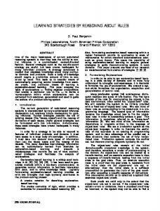
Example 2.2 (Paper, Rock, and Scissor). Consider the classic DA DB two-player concurrent game paper, rock, and scissor (PRS, for short) sA sB as represented in Figure 1, where a play continues until one of the wA wB participants catches the move of the other. Vertexes are states of the game and labels on edges represent decisions of agents or sets of ∗∗ ∗∗ them, where the symbol ∗ is used in place of every possible action. In Fig. 1: The C GS GPRS . this specific case, since there are only two agents, the pair of symbols ∗∗ indicates the whole set Dc of decisions. The agents “Alice” and “Bob” in Ag , {A, B} have as possible actions those in the set Ac , {P, R, S}, which stand for “paper”, “rock”, and “scissor”, respectively. During the play, the game can stay in one of the three states in St , {si , sA , sB }, which represent, respectively, the waiting moment, named idle, and the two winner positions. The latter ones are labeled with one of the atomic propositions in AP , {wA , wB }, in order to represent who is the winner. The catch of one action over another is described by the relation C , {(P, R), (R, S), (S, P)} ⊆ Ac × Ac. We can now define the C GS GPRS , hAP, Ag, Ac, St, λ, τ, si i for the PRS game, with the labeling given by λ(si ) , ∅, λ(sA ) , {wA }, and λ(sB ) , {wB } and the transition function set as follows, where DA , {d ∈ DcGPRS : (d(A), d(B)) ∈ C } and DB , {d ∈ DcGPRS : (d(B), d(A)) ∈ C } are the sets of winning decisions for the two agents: if s = si and d ∈ DA then τ (s, d) , sA , else if s = si and d ∈ DB then τ (s, d) , sB , otherwise τ (s, d) , s. Note that, when none of the two agents catches the action of the other, i.e., the used decision is in Di , DcGPRS \ (DA ∪ DB ), the play remains in the idle state to allow another try, otherwise it is stuck in a winning position forever.

1 In

the following, we use both X → Y and Y X to denote the set of functions from the domain X to the codomain Y.



We now describe a non-classic qualitative version of the wellknown prisoner’s dilemma.

CC

A:7

si

fA1 , fA2

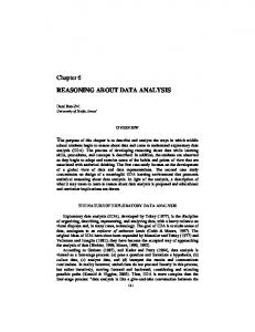
Example 2.3 (Prisoner’s Dilemma). In the prisoner’s dilemma DC CD (PD, for short), two accomplices are interrogated in separated rooms DD sA1 sA2 by the police, which offers them the same agreement. If one defects, fA1 fA2 i.e., testifies for the prosecution against the other, while the other cosj operates, i.e., remains silent, the defector goes free and the silent ac∅ ∗∗ ∗∗ complice goes to jail. If both cooperate, they remain free, but will ∗∗ be surely interrogated in the next future waiting for a defection. On the other hand, if every one defects, both go to jail. It is ensured Fig. 2: The C GS GPD . that no one will know about the choice made by the other. This tricky situation can be modeled by the C GS GPD , hAP, Ag, Ac, St, λ, τ, si i depicted in Figure 2, where the agents “Accomplice-1” and “Accomplice-2” in Ag , {A1 , A2 } can chose an action in Ac , {C, D}, which stand for “cooperation” and “defection”, respectively. There are four states in St , {si , sA1 , sA2 , sj }. In the idle state si the agents are waiting for the interrogation, while sj represents the jail for both of them. The remaining states sA1 and sA2 indicate, instead, the situations in which only one of the agents become definitely free. To characterize the different meaning of these states, we use the atomic propositions in AP , {fA1 , fA2 }, which denote who is “free”, by defining the following labeling: λ(si ) , {fA1 , fA2 }, λ(sA1 ) , {fA1 }, λ(sA2 ) , {fA2 }, and λ(sj ) , ∅. The transition function τ can be easily deduced by the figure. 2.2. Syntax

Strategy Logic (S L, for short) syntactically extends LTL by means of two strategy quantifiers, the existential hhxii and the universal [[x]], and agent binding (a, x), where a is an agent and x a variable. Intuitively, these new elements can be respectively read as “there exists a strategy x”, “for all strategies x”, and “bind agent a to the strategy associated with the variable x”. The formal syntax of S L follows. Definition 2.4 (S L Syntax). S L formulas are built inductively from the sets of atomic propositions AP, variables Var, and agents Ag, by using the following grammar, where p ∈ AP, x ∈ Var, and a ∈ Ag: ϕ ::= p | ¬ϕ | ϕ ∧ ϕ | ϕ ∨ ϕ | X ϕ | ϕ U ϕ | ϕ R ϕ | hhxiiϕ | [[x]]ϕ | (a, x)ϕ. S L denotes the infinite set of formulas generated by the above rules. Observe that, by construction, LTL is a proper syntactic fragment of S L, i.e., LTL ⊂ S L. In order to abbreviate the writing of formulas, we use the boolean values true t and false f and the well-known temporal operators future F ϕ , t U ϕ and globally G ϕ , f R ϕ. Moreover, we use the italic letters x, y, z, . . ., possibly with indexes, as meta-variables on the variables x, y, z, . . . in Var. A first classic notation related to the S L syntax that we need to introduce is that of subformula, i.e., a syntactic expression that is part of an a priori given formula. By sub : S L → 2SL we formally denote the function returning the set of subformulas of an S L formula. For instance, consider ϕ = hhxii(α, x)(F p). Then, it is immediate to see that sub(ϕ) = {ϕ, (α, x)(F p), (F p), p, t}. Normally, predicative logics need the concepts of free and bound placeholders in order to formally define the meaning of their formulas. The placeholders are used to represent particular positions in syntactic expressions that have to be highlighted, since they have a crucial role in the definition of the semantics. In first order logic, for instance, there is only one type of placeholders, which is represented by the variables. In S L, instead, we have both agents and variables as placeholders, as it can be noted by its syntax, in order to distinguish between the quantification of a strategy and its application by an agent. Consequently, we need a way to differentiate if an agent has an associated strategy via a variable and if a variable is quantified. To do this, we use the set of free ACM Journal Name, Vol. V, No. N, Article A, Publication date: January YYYY.

A:8


agents/variables as the subset of Ag ∪ Var containing (i) all agents for which there is no binding after the occurrence of a temporal operator and (ii) all variables for which there is a binding but no quantifications. Definition 2.5 (S L Free Agents/Variables). The set of free agents/variables of an S L formula is given by the function free : S L → 2Ag∪Var defined as follows: (i) (ii) (iii) (iv) (v) (vi) (vii) (viii)

free(p) , ∅, where p ∈ AP; free(¬ϕ) , free(ϕ); free(ϕ1 Op ϕ2 ) , free(ϕ1 ) ∪ free(ϕ2 ), where Op ∈ {∧, ∨}; free(X ϕ) , Ag ∪ free(ϕ); free(ϕ1 Op ϕ2 ) , Ag ∪ free(ϕ1 ) ∪ free(ϕ2 ), where Op ∈ {U, R}; free(Qn ϕ) , free(ϕ) \ {x}, where Qn ∈ {hhxii, [[x]] : x ∈ Var}; free((a, x)ϕ) , free(ϕ), if a 6∈ free(ϕ), where a ∈ Ag and x ∈ Var; free((a, x)ϕ) , (free(ϕ) \ {a}) ∪ {x}, if a ∈ free(ϕ), where a ∈ Ag and x ∈ Var.

A formula ϕ without free agents (resp., variables), i.e., with free(ϕ)∩Ag = ∅ (resp., free(ϕ)∩Var = ∅), is named agent-closed (resp., variable-closed). If ϕ is both agent- and variable-closed, it is referred to as a sentence. The function snt : S L → 2SL returns the set of subsentences snt(ϕ) , {φ ∈ sub(ϕ) : free(φ) = ∅} for each S L formula ϕ. Observe that, on one hand, free agents are introduced in Items iv and v and removed in Item viii. On the other hand, free variables are introduced in Item viii and removed in Item vi. As an example, let ϕ = hhxii(α, x)(β, y)(F p) be a formula on the agents Ag = {α, β, γ}. Then, we have free(ϕ) = {γ, y}, since γ is an agent without any binding after F p and y has no quantification at all. Consider also the formulas (α, z)ϕ and (γ, z)ϕ, where the subformula ϕ is the same as above. Then, we have free((α, z)ϕ) = free(ϕ) and free((γ, z)ϕ) = {y, z}, since α is not free in ϕ but γ is, i.e., α ∈ / free(ϕ) and γ ∈ free(ϕ). So, (γ, z)ϕ is agent-closed while (α, z)ϕ is not. Similarly to the case of first order logic, another important concept that characterizes the syntax of S L is that of the alternation number of quantifiers, i.e., the maximum number of quantifier switches hh·ii[[·]], [[·]]hh·ii, hh·ii¬hh·ii, or [[·]]¬[[·]] that bind a variable in a subformula that is not a sentence. The constraint on the kind of subformulas that are considered here means that, when we evaluate the number of such switches, we consider each possible subsentence as an atomic proposition, hence, its quantifiers are not taken into account. Moreover, it is important to observe that vacuous quantifications, i.e., quantifications on variable that are not free in the immediate inner subformula, need to be not considered at all in the counting of quantifier switches. This value is crucial when we want to analyze the complexity of the decision problems of fragments of our logic, since higher alternation can usually mean higher complexity. By alt : S L → N we formally denote the function returning the alternation number of an S L formula. Furthermore, the fragment S L[k-alt] , {ϕ ∈ S L : ∀ϕ′ ∈ sub(ϕ) . alt(ϕ′ ) ≤ k} of S L, for k ∈ N, denotes the subset of formulas having all subformulas with alternation number bounded by k. For instance, consider the sentence ϕ = [[x]]hhyii(α, x)(β, y)(F ϕ′ ) with ϕ′ = [[x]]hhyii(α, x)(β, y)(X p), on the set of agents Ag = {α, β}. Then, the alternation number alt(ϕ) is 1 and not 3, as one can think at a first glance, since ϕ′ is a sentence. Moreover, it holds that alt(ϕ′ ) = 1. Hence, ϕ ∈ S L[1-alt]. On the other hand, if we substitute ϕ′ with ϕ′′ = [[x]](α, x)(X p), we have that alt(ϕ) = 2, since ϕ′′ is not a sentence. Thus, it holds that ϕ 6∈ S L[1-alt] but ϕ ∈ S L[2-alt]. At this point, in order to practice with the syntax of our logic by expressing game-theoretic concepts through formulas, we describe two examples of important properties that are possible to write in S L, but neither in ATL∗ [Alur et al. 2002] nor in CHP-S L. This is clarified later in the paper. The first concept we introduce is the well-known deterministic concurrent multi-player Nash equilibrium for Boolean valued payoffs. ACM Journal Name, Vol. V, No. N, Article A, Publication date: January YYYY.


A:9

Example 2.6 (Nash Equilibrium). Consider the n agents α1 , . . . , αn of a game, each of them having, respectively, a possibly different temporal goal described by one of the LTL formulas ψ1 ,. . ., ψn . Then, we can express the existence of a strategy profile (x1 , . . . , xn ) that is a Nash equilibrium (NE, for short) for α1 , . . . , αn w.r.t. ψ1V , . . . , ψn by using the S L[1-alt] sentence ϕNE , hhx1 ii(α1 , x1 ) · · · hhxn ii(αn , xn ) ψNE , where ψNE , ni=1 (hhyii(αi , y)ψi ) → ψi is a variable-closed formula. Informally, this asserts that every agent αi has xi as one of the best strategy w.r.t. the goal ψi , once all the other strategies of the remaining agents αj , with j 6= i, have been fixed to xj . Note that here we are only considering equilibria under deterministic strategies. As in physics, also in game theory an equilibrium is not always stable. Indeed, there are games like the PD of Example 2.3 on page 7 having Nash equilibria that are instable. One of the simplest concepts of stability that is possible to think is called stability profile. Example 2.7 (Stability Profile). Think about the same situation of the above example on NE. Then, a stability profile (SP, for short) is a strategy profile (x1 , . . . , xn ) for α1 , . . . , αn w.r.t. ψ1 , . . . , ψn such that there is no agent αi that can choose a different strategy from xi without changing its own payoff and penalizing the payoff of another agent αj , with j 6= i. To represent the existence of such a profile, we can use the S L[1-alt] sentence ϕSP , hhx1 ii(α1 , x1 ) · · · hhxn ii(αn , xn )ψSP , Vn where ψSP , i,j=1,i6=j ψj → [[y]]((ψi ↔ (αi , y)ψi ) → (αi , y)ψj ). Informally, with the ψSP subformula, we assert that, if αj is able to achieve his goal ψj , all strategies y of αi that left unchanged the payoff related to ψi , also let αj to maintain his achieved goal. At this point, it is very easy to ensure the existence of an NE that is also an SP, by using the S L[1-alt] sentence ϕSNE , hhx1 ii(α1 , x1 ) · · · hhxn ii(αn , xn ) ψSP ∧ ψNE . 2.3. Basic concepts

Before continuing with the description of our logic, we have to introduce some basic concepts, regarding a generic C GS, that are at the base of the semantics formalization. Remind that a description of used mathematical notation is reported in Appendix A. We start with the notions of track and path. Intuitively, tracks and paths of a C GS G are legal sequences of reachable states in G that can be respectively seen as partial and complete descriptions of possible outcomes of the game modeled by G itself. Definition 2.8 (Tracks and Paths). A track (resp., path) in a C GS G is a finite (resp., an infinite) sequence of states ρ ∈ St∗ (resp., π ∈ Stω ) such that, for all i ∈ [0, |ρ| − 1[ (resp., i ∈ N), there exists a decision d ∈ Dc such that (ρ)i+1 = τ ((ρ)i , d) (resp., (π)i+1 = τ ((π)i , d)). 2 A track ρ is non-trivial if it has non-zero length, i.e., |ρ| > 0 that is ρ 6= ε. 3 The set Trk ⊆ St+ (resp., Pth ⊆ Stω ) contains all non-trivial tracks (resp., paths). Moreover, Trk(s) , {ρ ∈ Trk : fst(ρ) = s} (resp., Pth(s) , {π ∈ Pth : fst(π) = s}) indicates the subsets of tracks (resp., paths) starting at a state s ∈ St. 4 For instance, consider the PRS game of Example 2.2 on page 6. Then, ρ = si · sA ∈ St+ and π = si ω ∈ Stω are, respectively, a track and a path in the C GS GPRS . Moreover, it holds that Trk = si + + si ∗ · (sA + + sB + ) and Pth = si ω + si ∗ · (sA ω + sB ω ). At this point, we can define the concept of strategy. Intuitively, a strategy is a scheme for an agent that contains all choices of actions as a function of the history of the current outcome. However, observe that here we do not set an a priori connection between a strategy and an agent, since the same strategy can be used by more than one agent at the same time. notation (w)i ∈ Σ indicates the element of index i ∈ [0, |w|[ of a non-empty sequence w ∈ Σ∞ . Greek letter ε stands for the empty sequence. 4 By fst(w) , (w) it is denoted the first element of a non-empty sequence w ∈ Σ∞ . 0

2 The

3 The


A:10


Definition 2.9 (Strategies). A strategy in a C GS G is a partial function f : Trk ⇀ Ac that maps each non-trivial track in its domain to an action. For a state s ∈ St, a strategy f is said s-total if it is defined on all tracks starting in s, i.e., dom(f) = Trk(s). The set Str , Trk ⇀ Ac (resp., Str(s) , Trk(s) → Ac) contains all (resp., s-total) strategies. An example of strategy in the C GS GPRS is the function f1 ∈ Str(si ) that maps each track having length multiple of 3 to the action P, the tracks whose remainder of length modulo 3 is 1 to the action R, and the remaining tracks to the action S. A different strategy is given by the function f2 ∈ Str(si ) that returns the action P, if the tracks ends in sA or sB or if its length is neither a second nor a third power of a positive number, the action R, if the length is a square power, and the action S, otherwise. An important operation on strategies is that of translation along a given track, which is used to determine which part of a strategy has yet to be used in the game. Definition 2.10 (Strategy Translation). Let f ∈ Str be a strategy and ρ ∈ dom(f) a track in its domain. Then, (f)ρ ∈ Str denotes the translation of f along ρ, i.e., the strategy with dom((f)ρ ) , {ρ′ ∈ Trk(lst(ρ)) : ρ · ρ′≥1 ∈ dom(f)} such that (f)ρ (ρ′ ) , f(ρ · ρ′≥1 ), for all ρ′ ∈ dom((f)ρ ). 5 6 Intuitively, the translation (f)ρ is the update of the strategy f, once the history of the game becomes ρ. It is important to observe that, if f is a fst(ρ)-total strategy then (f)ρ is lst(ρ)-total. For instance, consider the two tracks ρ1 = si 4 ∈ Trk(si ) and ρ2 = si 4 · sA 2 ∈ Trk(si ) in the C GS GPRS and the strategy f1 ∈ Str(si ) previously described. Then, we have that (f1 )ρ1 = f1 , while (f1 )ρ2 ∈ Str(sA ) maps each track having length multiple of 3 to the action S, each track whose remainder of length modulo 3 is 1 to the action P, and the remaining tracks to the action R. We now introduce the notion of assignment. Intuitively, an assignment gives a valuation of variables with strategies, where the latter are used to determine the behavior of agents in the game. With more detail, as in the case of first order logic, we use this concept as a technical tool to quantify over strategies associated with variables, independently of agents to which they are related to. So, assignments are used precisely as a way to define a correspondence between variables and agents via strategies. Definition 2.11 (Assignments). An assignment in a C GS G is a partial function χ : Var ∪ Ag ⇀ Str mapping variables and agents in its domain to a strategy. An assignment χ is complete if it is defined on all agents, i.e., Ag ⊆ dom(χ). For a state s ∈ St, it is said that χ is s-total if all strategies χ(l) are s-total, for l ∈ dom(χ). The set Asg , Var ∪ Ag ⇀ Str (resp., Asg(s) , Var ∪ Ag ⇀ Str(s)) contains all (resp., s-total) assignments. Moreover, Asg(X) , X → Str (resp., Asg(X, s) , X → Str(s)) indicates the subset of X-defined (resp., s-total) assignments, i.e., (resp., s-total) assignments defined on the set X ⊆ Var ∪ Ag. As an example of assignment, let us consider the function χ1 ∈ Asg in the C GS GPRS , defined on the set {A, x}, whose values are f1 on A and f2 on x, where the strategies f1 , f2 ∈ Str(si ) are those described above. Another examples is given by the assignment χ2 ∈ Asg, defined on the set {A, B}, such that χ2 (A) = χ1 (x) and χ2 (B) = χ1 (A). Note that both are si -total and the latter is also complete while the former is not. As in the case of strategies, it is useful to define the operation of translation along a given track for assignments too. Definition 2.12 (Assignment Translation). For a given state s ∈ St, let χ ∈ Asg(s) be an stotal assignment and ρ ∈ Trk(s) a track. Then, (χ)ρ ∈ Asg(lst(ρ)) denotes the translation of χ along ρ, i.e., the lst(ρ)-total assignment, with dom((χ)ρ ) , dom(χ), such that (χ)ρ (l) , (χ(l))ρ , for all l ∈ dom(χ). 5 By

lst(w) , (w)|w|−1 it is denoted the last element of a finite non-empty sequence w ∈ Σ∗ . notation (w)≥i ∈ Σ∞ indicates the suffix from index i ∈ [0, |w|] inwards of a non-empty sequence w ∈ Σ∞ .

6 The



A:11

Intuitively, the translation (χ)ρ is the simultaneous update of all strategies χ(l) defined by the assignment χ, once the history of the game becomes ρ. Given an assignment χ, an agent or variable l, and a strategy f, it is important to define a notation to represent the redefinition of χ, i.e., a new assignment equal to the first on all elements of its domain but l, on which it assumes the value f. Definition 2.13 (Assignment Redefinition). Let χ ∈ Asg be an assignment, f ∈ Str a strategy and l ∈ Var ∪ Ag either an agent or a variable. Then, χ[l 7→ f] ∈ Asg denotes the new assignment defined on dom(χ[l 7→ f]) , dom(χ) ∪ {l} that returns f on l and is equal to χ on the remaining part of its domain, i.e., χ[l 7→ f](l) , f and χ[l 7→ f](l′ ) , χ(l′ ), for all l′ ∈ dom(χ) \ {l}. Intuitively, if we have to add or update a strategy that needs to be bound by an agent or variable, we can simply take the old assignment and redefine it by using the above notation. It is worth to observe that, if χ and f are s-total then χ[l 7→ f] is s-total too. Now, we can introduce the concept of play in a game. Intuitively, a play is the unique outcome of the game determined by all agent strategies participating to it. Definition 2.14 (Plays). A path π ∈ Pth(s) starting at a state s ∈ St is a play w.r.t. a complete s-total assignment χ ∈ Asg(s) ((χ, s)-play, for short) if, for all i ∈ N, it holds that (π)i+1 = τ ((π)i , d), where d(a) , χ(a)((π)≤i ), for each a ∈ Ag. 7 The partial function play : Asg × St ⇀ Pth, with dom(play) , {(χ, s) : Ag ⊆ dom(χ) ∧ χ ∈ Asg(s) ∧ s ∈ St}, returns the (χ, s)-play play(χ, s) ∈ Pth(s), for all pairs (χ, s) in its domain. As a last example, consider again the complete si -total assignment χ2 previously described for the C GS GPRS , which returns the strategies f2 and f1 on the agents A and B, respectively. Then, we have that play(χ2 , si ) = si 3 · sB ω . This means that the play is won by the agent B. Finally, we give the definition of global translation of a complete assignment together with a related state, which is used to calculate, at a certain step of the play, what is the current state and its updated assignment. Definition 2.15 (Global Translation). For a given state s ∈ St and a complete s-total assignment χ ∈ Asg(s), the i-th global translation of (χ, s), with i ∈ N, is the pair of a complete assignment and a state (χ, s)i , ((χ)(π)≤i , (π)i ), where π = play(χ, s). In order to avoid any ambiguity of interpretation of the described notions, we may use the name of a C GS as a subscript of the sets and functions just introduced to clarify to which structure they are related to, as in the case of components in the tuple-structure of the C GS itself. 2.4. Semantics

As already reported at the beginning of this section, just like ATL∗ and differently from CHP-S L, the semantics of S L is defined w.r.t. concurrent game structures. For a C GS G, one of its states s, and an s-total assignment χ with free(ϕ) ⊆ dom(χ), we write G, χ, s |= ϕ to indicate that the formula ϕ holds at s in G under χ. The semantics of S L formulas involving the atomic propositions, the Boolean connectives ¬, ∧, and ∨, as well as the temporal operators X, U, and R is defined as usual in LTL. The novel part resides in the formalization of the meaning of strategy quantifications hhxii and [[x]] and agent binding (a, x). Definition 2.16 (S L Semantics). Given a C GS G, for all S L formulas ϕ, states s ∈ St, and s-total assignments χ ∈ Asg(s) with free(ϕ) ⊆ dom(χ), the modeling relation G, χ, s |= ϕ is inductively defined as follows. (1) G, χ, s |= p if p ∈ λ(s), with p ∈ AP. (2) For all formulas ϕ, ϕ1 , and ϕ2 , it holds that: 7 The

notation (w)≤i ∈ Σ∗ indicates the prefix up to index i ∈ [0, |w|] of a non-empty sequence w ∈ Σ∞ .


A:12


(a) G, χ, s |= ¬ϕ if not G, χ, s |= ϕ, that is G, χ, s 6|= ϕ; (b) G, χ, s |= ϕ1 ∧ ϕ2 if G, χ, s |= ϕ1 and G, χ, s |= ϕ2 ; (c) G, χ, s |= ϕ1 ∨ ϕ2 if G, χ, s |= ϕ1 or G, χ, s |= ϕ2 . (3) For a variable x ∈ Var and a formula ϕ, it holds that: (a) G, χ, s |= hhxiiϕ if there exists an s-total strategy f ∈ Str(s) such that G, χ[x 7→ f], s |= ϕ; (b) G, χ, s |= [[x]]ϕ if for all s-total strategies f ∈ Str(s) it holds that G, χ[x 7→ f], s |= ϕ. (4) For an agent a ∈ Ag, a variable x ∈ Var, and a formula ϕ, it holds that G, χ, s |= (a, x)ϕ if G, χ[a 7→ χ(x)], s |= ϕ. (5) Finally, if the assignment χ is also complete, for all formulas ϕ, ϕ1 , and ϕ2 , it holds that: (a) G, χ, s |= X ϕ if G, (χ, s)1 |= ϕ; (b) G, χ, s |= ϕ1 U ϕ2 if there is an index i ∈ N with k ≤ i such that G, (χ, s)i |= ϕ2 and, for all indexes j ∈ N with k ≤ j < i, it holds that G, (χ, s)j |= ϕ1 ; (c) G, χ, s |= ϕ1 R ϕ2 if, for all indexes i ∈ N with k ≤ i, it holds that G, (χ, s)i |= ϕ2 or there is an index j ∈ N with k ≤ j < i such that G, (χ, s)j |= ϕ1 . Intuitively, at Items 3a and 3b, respectively, we evaluate the existential hhxii and universal [[x]] quantifiers over strategies, by associating them to the variable x. Moreover, at Item 4, by means of an agent binding (a, x), we commit the agent a to a strategy associated with the variable x. It is evident that, due to Items 5a, 5b, and 5c, the LTL semantics is simply embedded into the S L one. In order to complete the description of the semantics, we now give the classic notions of model and satisfiability of an S L sentence. Definition 2.17 (S L Satisfiability). We say that a C GS G is a model of an S L sentence ϕ, in symbols G |= ϕ, if G, ∅, s0 |= ϕ. 8 In general, we also say that G is a model for ϕ on s ∈ St, in symbols G, s |= ϕ, if G, ∅, s |= ϕ. An S L sentence ϕ is satisfiable if there is a model for it. It remains to introduce the concepts of implication and equivalence between S L formulas, which are useful to describe transformations preserving the meaning of a specification. Definition 2.18 (S L Implication and Equivalence). Given two S L formulas ϕ1 and ϕ2 with free(ϕ1 ) = free(ϕ2 ), we say that ϕ1 implies ϕ2 , in symbols ϕ1 ⇒ ϕ2 , if, for all C GSs G, states s ∈ St, and free(ϕ1 )-defined s-total assignments χ ∈ Asg(free(ϕ1 ), s), it holds that if G, χ, s |= ϕ1 then G, χ, s |= ϕ2 . Accordingly, we say that ϕ1 is equivalent to ϕ2 , in symbols ϕ1 ≡ ϕ2 , if both ϕ1 ⇒ ϕ2 and ϕ2 ⇒ ϕ1 hold. In the rest of the paper, especially when we describe a decision procedure, we may consider formulas in existential normal form (enf, for short) and positive normal form (pnf, for short), i.e., formulas in which only existential quantifiers appear or in which the negation is applied only to atomic propositions. In fact, it is to this aim that we have considered in the syntax of S L both the Boolean connectives ∧ and ∨, the temporal operators U, and R, and the strategy quantifiers hh·ii and [[·]]. Indeed, all formulas can be linearly translated in pnf by using De Morgan’s laws together with the following equivalences, which directly follow from the semantics of the logic: ¬X ϕ ≡ X ¬ϕ, ¬(ϕ1 U ϕ2 ) ≡ (¬ϕ1 )R (¬ϕ2 ), ¬hhxiiϕ ≡ [[x]]¬ϕ, and ¬(a, x)ϕ ≡ (a, x)¬ϕ. 11 At this point, in order to better understand the meaning of our logic, we discuss two examples in which we describe the evaluation s0 ∅ of the semantics of some formula w.r.t. the a priori given C GSs. We start by explaining how a strategy can be shared by different agents. ∗∗ 10 00

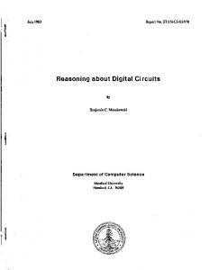
Example 2.19 (Shared Variable). Consider the S L[2-alt] sentence ϕ = hhxii[[y]]hhzii((α, x)(β, y)(X p) ∧ (α, y)(β, z)(X q)). It is immediate to note that both agents α and β use the strategy associated with y to achieve simultaneously the LTL temporal goals X p

∗∗ 01

∗∗

s1

s3

p

q

s2

p, q

Fig. 3: The C GS GSV . 8 The

symbol ∅ stands for the empty function.



A:13

and X q. A model for ϕ is given by the C GS GSV , h{p, q}, {α, β}, {0, 1}, {s0, s1 , s2 , s3 }, λ, τ, s0 i, where λ(s0 ) , ∅, λ(s1 ) , {p}, λ(s2 ) , {p, q}, λ(s3 ) , {q}, τ (s0 , (0, 0)) , s1 , τ (s0 , (0, 1)) , s2 , τ (s0 , (1, 0)) , s3 , and all the remaining transitions (with any decision) go to s0 . In Figure 3 on the facing page, we report a graphical representation of the structure. Clearly, GSV |= ϕ by letting, on s0 , the variables x to chose action 0 (the goal (α, x)(β, y)(X p) is satisfied for any choice of y, since we can move from s0 to either s1 or s2 , both labeled with p) and z to choose action 1 when y has action 0 and, vice versa, 0 when y has 1 (in both cases, the goal (α, y)(β, z)(X q) is satisfied, since one can move from s0 to either s2 or s3 , both labeled with q). We now discuss an application of the concepts of Nash equilibrium and stability profile to both the prisoner’s dilemma and the paper, rock, and scissor game. Example 2.20 (Equilibrium Profiles). Let us first to consider the C GS GPD of the prisoner’s dilemma described in the Example 2.3 on page 7. Intuitively, each of the two accomplices A1 and A2 want to avoid the prison. These goals can be, respectively, represented by the LTL formulas ψA1 , G fA1 and ψA2 , G fA2 . The existence of a Nash equilibrium in GPD for the two accomplices w.r.t. the above goals can be written as φNE , hhx1 ii(A1 , x1 )hhx2 ii(A2 , x2 ) ψNE , where ψNE , ((hhyii(A1 , y)ψA1 ) → ψA1 ) ∧ ((hhyii(A2 , y)ψA2 ) → ψA2 ), which results to be an instantiation of the general sentence ϕNE of Example 2.6 on page 9. In the same way, the existence of a stable Nash equilibrium can be represented with the sentence φSNE , hhx1 ii(A1 , x1 )hhx2 ii(A2 , x2 ) ψNE ∧ ψSP , where ψSP , (ψ1 → [[y]]((ψ2 ↔ (A2 , y)ψ2 ) → (A2 , y)ψ1 )) ∧ (ψ2 → [[y]]((ψ1 ↔ (A1 , y)ψ1 ) → (A1 , y)ψ2 )), which is a particular case of the sentence ϕSNE of Example 2.7 on page 9. Now, it is easy to see that GPD |= φSNE and, so, GPD |= φNE . Indeed, an assignment χ ∈ AsgGPD (Ag, si ), for which χ(A1 )(si ) = χ(A2 )(si ) = D, is a stable equilibrium profile, i.e., it is such that GPD , χ, si |= ψNE ∧ ψSP . This is due to the fact that, if an agent Ak , for k ∈ {1, 2}, choses another strategy f ∈ StrGPD (si ), he is still unable to achieve his goal ψk , i.e., GPD , χ[Ak 7→ f], si 6|= ψk , so, he cannot improve his payoff. Moreover, this equilibrium is stable, since the payoff of an agent cannot be made worse by the changing of the strategy of the other agent. However, it is interesting to note that there are instable equilibria too. One of these is represented by the assignment χ′ ∈ AsgGPD (Ag, si ), for which χ′ (A1 )(si j ) = χ′ (A2 )(si j ) = C, for all j ∈ N. Indeed, we have that GPD , χ′ , si |= ψNE , since GPD , χ′ , si |= ψ1 and GPD , χ′ , si |= ψ2 , but GPD , χ′ , si 6|= ψSP . The latter property holds because, if one of the agents Ak , for k ∈ {1, 2}, choses a different strategy f ′ ∈ StrGPD (si ) for which there is a j ∈ N such that f ′ (si j ) = D, he cannot improve his payoff but makes surely worse the payoff of the other agent, i.e., GPD , χ′ [Ak 7→ f ′ ], si |= ψk but GPD , χ′ [Ak 7→ f ′ ], si 6|= ψ3−k . Finally, consider the C GS GPRS of the paper, rock, and scissor game described in the Example 2.2 on page 6 together with the associated formula for the Nash equilibrium φNE , hhx1 ii(A, x1 )hhx2 ii(B, x2 ) ψNE , where ψNE , ((hhyii(A, y)ψA ) → ψA ) ∧ ((hhyii(B, y)ψB ) → ψB ) with ψA , F wA and ψB , F wB representing the LTL temporal goals for Alice and Bob, respectively. Then, it is not hard to see that GPRS 6|= φNE , i.e., there are no Nash equilibria in this game, since there is necessarily an agent that can improve his/her payoff by changing his/her strategy. Finally, we want to remark that our semantics framework, based on concurrent game structures, is enough expressive to describe turn-based features in the multi-agent case too. This is possible by simply allowing the transition function to depend only on the choice of actions of an a priori given agent for each state. Definition 2.21 (Turn-Based Game Structures). A C GS G is turn-based if there exists a function η : St → Ag, named owner function, such that, for all states s ∈ St and decisions d1 , d2 ∈ Dc, it holds that if d1 (η(s)) = d2 (η(s)) then τ (s, d1 ) = τ (s, d2 ). Intuitively, a C GS is turn-based if it is possible to associate with each state an agent, i.e., the owner of the state, which is responsible for the choice of the successor of that state. It is immediate to observe that η introduces a partitioning of the set of states into |rng(η)| components, each one ruled ACM Journal Name, Vol. V, No. N, Article A, Publication date: January YYYY.

A:14


by a single agent. Moreover, observe that a C GS having just one agent is trivially turn-based, since this agent is the only possible owner of all states. In the following, as one can expect, we also consider the case in which S L has its semantics defined on turn-based C GS only. In such an eventuality, we name the resulting semantic fragment Turn-based Strategy Logic (T B -S L, for short) and refer to the related satisfiability concept as turnbased satisfiability. 3. MODEL-CHECKING HARDNESS

In this section, we show the non-elementary lower bound for the model-checking problem of S L. Precisely, we prove that, for sentences having alternation number k, this problem is k-E XP S PACEHARD . To this aim, in Subsection 3.1, we first recall syntax and semantics of QP TL [Sistla 1983]. Then, in Subsection 3.2, we give a reduction from the satisfiability problem for this logic to the model-checking problem for S L. 3.1. Quantified propositional temporal logic

Quantified Propositional Temporal Logic (QP TL, for short) syntactically extends the old-style temporal logic with the future F and global G operators by means of two proposition quantifiers, the existential ∃q. and the universal ∀q., where q is an atomic proposition. Intuitively, these elements can be respectively read as “there exists an evaluation of q” and “for all evaluations of q”. The formal syntax of QP TL follows. Definition 3.1 (QP TL Syntax). QP TL formulas are built inductively from the sets of atomic propositions AP, by using the following grammar, where p ∈ AP: ϕ ::= p | ¬ϕ | ϕ ∧ ϕ | ϕ ∨ ϕ | X ϕ | F ϕ | G ϕ | ∃p.ϕ | ∀p.ϕ. QP TL denotes the infinite set of formulas generated by the above grammar. Similarly to S L, we use the concepts of subformula, free atomic proposition, sentence, and alternation number, together with the QP TL syntactic fragment of bounded alternation QP TL[k-alt], with k ∈ N. In order to define the semantics of QP TL, we have first to introduce the concepts of truth evaluations used to interpret the meaning of atomic propositions at the passing of time. Definition 3.2 (Truth Evaluations). A temporal truth evaluation is a function tte : N → {f, t} that maps each natural number to a Boolean value. Moreover, a propositional truth evaluation is a partial function pte : AP ⇀ TTE mapping every atomic proposition in its domain to a temporal truth evaluation. The sets TTE , N → {f, t} and PTE , AP ⇀ TTE contain, respectively, all temporal and propositional truth evaluations. At this point, we have the tool to define the interpretation of QP TL formulas. For a propositional truth evaluation pte with free(ϕ) ⊆ dom(pte) and a number k, we write pte, k |= ϕ to indicate that the formula ϕ holds at the k-th position of the pte. Definition 3.3 (QP TL Semantics). For all QP TL formulas ϕ, propositional truth evaluation pte ∈ PTE with free(ϕ) ⊆ dom(pte), and numbers k ∈ N, the modeling relation pte, k |= ϕ is inductively defined as follows. (1) pte, k |= p iff pte(p)(k) = t, with p ∈ AP. (2) For all formulas ϕ, ϕ1 , and ϕ2 , it holds that: (a) pte, k |= ¬ϕ iff not pte, k |= ϕ, that is pte, k 6|= ϕ; (b) pte, k |= ϕ1 ∧ ϕ2 iff pte, k |= ϕ1 and pte, k |= ϕ2 ; (c) pte, k |= ϕ1 ∨ ϕ2 iff pte, k |= ϕ1 or pte, k |= ϕ2 ; (d) pte, k |= X ϕ iff pte, k + 1 |= ϕ; (e) pte, k |= F ϕ iff there is an index i ∈ N with k ≤ i such that pte, i |= ϕ; ACM Journal Name, Vol. V, No. N, Article A, Publication date: January YYYY.


A:15

(f) pte, k |= G ϕ iff, for all indexes i ∈ N with k ≤ i, it holds that pte, i |= ϕ. (3) For an atomic proposition q ∈ AP and a formula ϕ, it holds that: (a) pte, k |= ∃q.ϕ iff there exists a temporal truth evaluation tte ∈ TTE such that pte[q 7→ tte], k |= ϕ; (b) pte, k |= ∀q.ϕ iff for all temporal truth evaluations tte ∈ TTE it holds that pte[q 7→ tte], k |= ϕ. Obviously, a QP TL sentence ϕ is satisfiable if ∅, 0 |= ϕ. Observe that the described semantics is slightly different but completely equivalent to that proposed and used in [Sistla et al. 1987] to prove the non-elementary hardness result for the satisfiability problem. 3.2. Non-elementary lower-bound

We can show how the solution of QP TL satisfiability problem can be reduced to that of the modelchecking problem for S L, over a turn-based constant size C GS with a unique atomic proposition. In order to do this, we first prove the following auxiliary lemma, f t which actually represents the main step of the above mentioned reduction. t s0

∅

s1

p

f L EMMA 3.4 (QP TL R EDUCTION ). There is a one-agent C GS GRdc such that, for each QP TL[k-alt] sentence ϕ, with k ∈ N, there exists Fig. 4: The C GS GRdc . an T B -S L[k-alt] variable-closed formula ϕ such that ϕ is satisfiable iff GRdc , χ, s0 |= ϕ, for all complete assignments χ ∈ Asg(Ag, s0 ).

P ROOF. Consider the one-agent C GS GRdc , h{p}, {α}, {f, t}, {s0, s1 }, λ, τ, s0 i depicted in Figure 4, where the two actions are the Boolean values false and true and where the labeling and transition functions λ and τ are set as follows: λ(s0 ) , ∅, λ(s1 ) , {p}, and τ (s, d) = s0 iff d(α) = f, for all s ∈ St and d ∈ Dc. It is evident that GRdc is a turn-based C GS. Moreover, consider the transformation function · : QP TL → S L inductively defined as follows: — q , (α, xq )X p, for q ∈ AP; — ∃q.ϕ , hhxq iiϕ; — ∀q.ϕ , [[xq ]]ϕ; — Op ϕ , Op ϕ, where Op ∈ {¬, X, F, G}; — ϕ1 Op ϕ2 , ϕ1 Op ϕ2 , where Op ∈ {∧, ∨}. It is not hard to see that a QP TL formula ϕ is a sentence iff ϕ is variable-closed. Furthermore, we have that alt(ϕ) = alt(ϕ). At this point, it remains to prove that, a QP TL sentence ϕ is satisfiable iff GRdc , χ, s0 |= ϕ, for all total assignments χ ∈ Asg({α}, s0 ). To do this by induction on the structure of ϕ, we actually show a stronger result asserting that, for all subformulas ψ ∈ sub(ϕ), propositional truth evaluations pte ∈ PTE, and i ∈ N, it holds that pte, i |= ψ iff GRdc , (χ, s0 )i |= ψ, for each total assignment χ ∈ Asg({α} ∪ {xq ∈ Var : q ∈ free(ψ)}, s0 ) such that χ(xq )((π)≤n ) = pte(q)(n), where π , play(χ, s0 ), for all q ∈ free(ψ) and n ∈ [i, ω[ . Here, we only show the base case of atomic propositions and the two inductive cases regarding the proposition quantifiers. The remaining cases of Boolean connectives and temporal operators are straightforward and left to the reader as a simple exercise. — ψ = q. By Item 1 of Definition 3.3 of QP TL semantics, we have that pte, i |= q iff pte(q)(i) = t. Thus, due to the above constraint on the assignment, it follows that pte, i |= q iff χ(xq )((π)≤i ) = t. Now, by applying Items 4 and 5a of Definition 2.16 of S L semantics, we have that GRdc , (χ, s0 )i |= (α, xq )X p iff GRdc , (χ′ [α 7→ χ′ (xq )], s′ )1 |= p, where (χ′ , s′ ) = (χ, s0 )i . At this point, due to the particular structure of the C GS GRdc , we have that GRdc , (χ′ [α 7→ χ′ (xq )], s′ )1 |= p iff (π ′ )1 = s1 , ACM Journal Name, Vol. V, No. N, Article A, Publication date: January YYYY.

A:16


where π ′ , play(χ′ [α 7→ χ′ (xq )], s′ ), which in turn is equivalent to χ′ (xq )((π ′ )≤0 ) = t. So, GRdc , (χ, s0 )i |= (α, xq )X p iff χ′ (xq )((π ′ )≤0 ) = t. Now, by observing that (π ′ )≤0 = (π)i and using the above definition of χ′ , we obtain that χ′ (xq )((π ′ )≤0 ) = χ(xq )((π)≤i ). Hence, pte, i |= q iff pte(q)(i) = χ(xq )((π)≤i ) = t = χ′ (xq )((π ′ )≤0 ) iff GRdc , (χ, s0 )i |= (α, xq )X p. — ψ = ∃q.ψ ′ . [Only if]. If pte, i |= ∃q.ψ ′ , by Item 3a of Definition 3.3, there exists a temporal truth evaluation tte ∈ TTE such that pte[q 7→ tte], i |= ψ ′ . Now, consider a strategy f ∈ Str(s0 ) such that f((π)≤n ) = tte(n), for all n ∈ [i, ω[ . Then, it is evident that χ[xq 7→ f](xq′ )((π)≤n ) = pte[q 7→ tte](q ′ )(n), for all q ′ ∈ free(ψ) and n ∈ [i, ω[ . So, by the inductive hypothesis, it follows that GRdc , (χ[xq 7→ f], s0 )i |= ψ ′ . Thus, we have that GRdc , (χ, s0 )i |= hhxq iiψ ′ . [If]. If GRdc , (χ, s0 )i |= hhxq iiψ ′ , there exists a strategy f ∈ Str(s0 ) such that GRdc , (χ[xq 7→ f], s0 )i |= ψ ′ . Now, consider a temporal truth evaluation tte ∈ TTE such that tte(n) = f((π)≤n ), for all n ∈ [i, ω[ . Then, it is evident that χ[xq 7→ f](xq′ )((π)≤n ) = pte[q 7→ tte](q ′ )(n), for all q ′ ∈ free(ψ) and n ∈ [i, ω[ . So, by the inductive hypothesis, it follows that pte[q 7→ tte], i |= ψ ′ . Thus, by Item 3a of Definition 3.3, we have that pte, i |= ∃q.ψ ′ . — ψ = ∀q.ψ ′ . [Only if]. For each strategy f ∈ Str(s0 ), consider a temporal truth evaluation tte ∈ TTE such that tte(n) = f((π)≤n ), for all n ∈ [i, ω[ . It is evident that χ[xq 7→ f](xq′ )((π)≤n ) = pte[q 7→ tte](q ′ )(n), for all q ′ ∈ free(ψ) and n ∈ [i, ω[ . Now, since pte, i |= ∀q.ψ ′ , by Item 3b of Definition 3.3, it follows that pte[q 7→ tte], i |= ψ ′ . So, by the inductive hypothesis, for each strategy f ∈ Str(s0 ), it holds that GRdc , (χ[xq 7→ f], s0 )i |= ψ ′ . Thus, we have that GRdc , (χ, s0 )i |= [[xq ]]ψ ′ . [If]. For each temporal truth evaluation tte ∈ TTE, consider a strategy f ∈ Str(s0 ) such that f((π)≤n ) = tte(n), for all n ∈ [i, ω[ . It is evident that χ[xq 7→ f](xq′ )((π)≤n ) = pte[q 7→ tte](q ′ )(n), for all q ′ ∈ free(ψ) and n ∈ [i, ω[. Now, since GRdc , (χ, s0 )i |= [[xq ]]ψ ′ , it follows that GRdc , (χ[xq 7→ f], s0 )i |= ψ ′ . So, by the inductive hypothesis, for each temporal truth evaluation tte ∈ TTE, it holds that pte[q 7→ tte], i |= ψ ′ . Thus, by Item 3b of Definition 3.3, we have that pte, i |= ∀q.ψ ′ . Thus, we are done with the proof. Now, we can show the full reduction that allows us to state the existence of a non-elementary lower-bound for the model-checking problem of T B -S L and, thus, of S L. T HEOREM 3.5 (T B -S L M ODEL -C HECKING H ARDNESS ). The model-checking problem for T B -S L[k-alt] is k-E XP S PACE-HARD. P ROOF. Let ϕ be a QP TL[k-alt] sentence, ϕ the related T B -S L[k-alt] variable-closed formula, and GRdc the turn-based C GS of Lemma 3.4 of QP TL reduction. Then, by applying the previous mentioned lemma, it is easy to see that ϕ is satisfiable iff GRdc |= [[x]](α, x)ϕ iff GRdc |= hhxii(α, x)ϕ. Thus, the satisfiability problem for QP TL can be reduced to the model-checking problem for T B -S L. Now, since the satisfiability problem for QP TL[k-alt] is k-E XP S PACE-HARD [Sistla et al. 1987], we have that the model-checking problem for T B -S L[k-alt] is k-E XP S PACE-HARD as well. The following corollary is an immediate consequence of the previous theorem. C OROLLARY 3.6 (S L M ODEL -C HECKING H ARDNESS ). S L[k-alt] is k-E XP S PACE-HARD.

The model-checking problem for

4. STRATEGY QUANTIFICATIONS

Since model checking for S L is non-elementary hard while the same problem for ATL∗ is only 2E XP T IME-COMPLETE, a question that naturally arises is whether there are proper fragments of S L of practical interest, still strictly subsuming ATL∗ , that reside in such a complexity gap. In this ACM Journal Name, Vol. V, No. N, Article A, Publication date: January YYYY.


A:17

section, we answer positively to this question and go even further. Precisely, we enlighten a fundamental property that, if satisfied, allows to retain a 2E XP T IME-COMPLETE model-checking problem. We refer to such a property as elementariness. To formally introduce this concept, we use the notion of dependence map as a machinery. The remaining part of this section is organized as follows. In Subsection 4.1, we describe three syntactic fragments of S L, named S L[NG], S L[BG], and S L[1 G], having the peculiarity to use strategy quantifications grouped in atomic blocks. Then, in Subsection 4.2, we define the notion of dependence map, which is used, in Subsection 4.3, to introduce the concept of elementariness. Finally, in Subsection 4.4, we prove a fundamental result, which is at the base of our elementary modelchecking procedure for S L[1 G]. 4.1. Syntactic fragments

In order to formalize the syntactic fragments of S L we want to investigate, we first need to define the concepts of quantification and binding prefixes. Definition 4.1 (Prefixes). A quantification prefix over a set V ⊆ Var of variables is a finite word ℘ ∈ {hhxii, [[x]] : x ∈ V}|V| of length |V| such that each variable x ∈ V occurs just once in ℘, i.e., there is exactly one index i ∈ [0, |V|[ such that (℘)i ∈ {hhxii, [[x]]}. A binding prefix over a set of variables V ⊆ Var is a finite word ♭ ∈ {(a, x) : a ∈ Ag ∧ x ∈ V}|Ag| of length |Ag| such that each agent a ∈ Ag occurs just once in ♭, i.e., there is exactly one index i ∈ [0, |Ag|[ for which (♭)i ∈ {(a, x) : x ∈ V}. Finally, Qnt(V) ⊆ {hhxii, [[x]] : x ∈ V}|V| and Bnd(V) ⊆ {(a, x) : a ∈ Ag ∧ x ∈ V}|Ag| denote, respectively, the sets of all quantification and binding prefixes over variables in V. We now have all tools to define the syntactic fragments we want to analyze, which we name, respectively, Nested-Goal, Boolean-Goal, and One-Goal Strategy Logic (S L[NG], S L[BG], and S L[1 G], for short). For goal we mean an S L agent-closed formula of the kind ♭ϕ, with Ag ⊆ free(ϕ), being ♭ ∈ Bnd(Var) a binding prefix. The idea behind S L[NG] is that, when there is a quantification over a variable used in a goal, we are forced to quantify over all free variables of the inner subformula containing the goal itself, by using a quantification prefix. In this way, the subformula is build only by nesting and Boolean combinations of goals. In addition, with S L[BG] we avoid nested goals sharing the variables of a same quantification prefix, but allow their Boolean combinations. Finally, S L[1 G] forces the use of a different quantification prefix for each single goal in the formula. The formal syntax of S L[NG], S L[BG], and S L[1 G] follows. Definition 4.2 (S L[NG], S L[BG], and S L[1 G] Syntax). S L[NG] formulas are built inductively from the sets of atomic propositions AP, quantification prefixes Qnt(V) for any V ⊆ Var, and binding prefixes Bnd(Var), by using the following grammar, with p ∈ AP, ℘ ∈ ∪V⊆Var Qnt(V), and ♭ ∈ Bnd(Var): ϕ ::= p | ¬ϕ | ϕ ∧ ϕ | ϕ ∨ ϕ | X ϕ | ϕ U ϕ | ϕ R ϕ | ℘ϕ | ♭ϕ, where in the formation rule ℘ϕ it is ensured that ϕ is agent-closed and ℘ ∈ Qnt(free(ϕ)). In addition, S L[BG] formulas are determined by splitting the above syntactic class in two different parts, of which the second is dedicated to build the Boolean combinations of goals avoiding their nesting: ϕ ::= p | ¬ϕ | ϕ ∧ ϕ | ϕ ∨ ϕ | X ϕ | ϕ U ϕ | ϕ R ϕ | ℘ψ, ψ ::= ♭ϕ | ¬ψ | ψ ∧ ψ | ψ ∨ ψ, where in the formation rule ℘ψ it is ensured that ℘ ∈ Qnt(free(ψ)). Finally, the simpler S L[1 G] formulas are obtained by forcing each goal to be coupled with a quantification prefix: ϕ ::= p | ¬ϕ | ϕ ∧ ϕ | ϕ ∨ ϕ | X ϕ | ϕ U ϕ | ϕ R ϕ | ℘♭ϕ, ACM Journal Name, Vol. V, No. N, Article A, Publication date: January YYYY.

A:18


where in the formation rule ℘♭ϕ it is ensured that ℘ ∈ Qnt(free(♭ϕ)). S L ⊃ S L[NG] ⊃ S L[BG] ⊃ S L[1 G] denotes the syntactic chain of infinite sets of formulas generated by the respective grammars with the associated constraints on free variables of goals. Intuitively, in S L[NG], S L[BG], and S L[1 G], we force the writing of formulas to use atomic blocks of quantifications and bindings, where the related free variables are strictly coupled with those that are effectively quantified in the prefix just before the binding. In a nutshell, we can only write formulas by using sentences of the form ℘ψ belonging to a kind of prenex normal form in which the quantifications contained into the matrix ψ only belong to the prefixes ℘′ of some inner subsentence ℘′ ψ ′ ∈ snt(℘ψ). An S L[NG] sentence φ is principal if it is of the form φ = ℘ψ, where ψ is agent-closed and ℘ ∈ Qnt(free(ψ)). By psnt(ϕ) ⊆ snt(ϕ) we denote the set of all principal subsentences of the formula ϕ. We now introduce other two general restrictions in which the numbers |Ag| of agents and |Var| of variables that are used to write a formula are fixed to the a priori values n, m ∈ [1, ω[ , respectively. Moreover, we can also forbid the sharing of variables, i.e., each variable is binded to one agent only, so, we cannot force two agents to use the same strategy. We name these three fragments S L[n-ag], S L[m-var], and S L[fvs], respectively. Note that, in the one agent fragment, the restriction on the sharing of variables between agents, naturally, does not act, i.e., S L[1-ag, fvs] = S L[1-ag]. To start to practice with the above fragments, consider again the sentence ϕ of Example 2.19 on page 12. It is easy to see that it actually belongs to S L[BG, 2-ag, 3-var, 2-alt], and so, to S L[NG], but not to S L[1 G], since it is of the form ℘(♭1 X p ∧ ♭2 X q), where the quantification prefix is ℘ = hhxii[[y]]hhzii and the binding prefixes of the two goals are ♭1 = (α, x)(β, y) and ♭2 = (α, y)(β, z). Along the paper, sometimes we assert that a given formula ϕ belongs to an S L syntactic fragment also if its syntax does not precisely correspond to what is described by the relative grammar. We do this in order to make easier the reading and interpretation of the formula ϕ itself and only in the case that it is simple to translate it into an equivalent formula that effectively belongs to the intended logic, by means of a simple generalization of classic rules used to put a formula of first order logic in the prenex normal form. For example, consider the sentence ϕNE of Example 2.6 on page 9 representing the existence of a Nash equilibrium. This formula is considered to V belong to S L[BG, n-ag, 2n-var, fvs, 1-alt], since it can be easily translated in the form n φNE = ℘ i=1 ♭i ψi → ♭ψi , where ℘ = hhx1 ii · · · hhxn ii[[y1 ]] · · · [[yn ]], ♭ = (α1 , x1 ) · · · (αn , xn ), ♭i = (α1 , x1 ) · · · (αi−1 , xi−1 )(αi , yi )(αi+1 , xi+1 ) · · · (αn , xn ), and free(ψi ) = Ag. As another example, consider the sentence ϕSP of Example 2.7 on page 9 representing the existence of a stability profile. Also this formula is considered to belong to S L[BG, n-ag, 2n-var, fvs, 1-alt], since it is equivVn alent to φSP = ℘ i,j=1,i6=j ♭ψj → ((♭ψi ↔ ♭i ψi ) → ♭i ψj ). Note that both φNE and φSP are principal sentences. Now, it is interesting to observe that C TL∗ and ATL∗ are exactly equivalent to S L[1 G, fvs, 0-alt] and S L[1 G, fvs, 1-alt], respectively. Moreover, G L [Alur et al. 2002] is the very simple fragment of S L[BG, fvs, 1-alt] that forces all goals in a formula to have a common part containing all variables quantified before the unique possible alternation of the quantification prefix. Finally, we have that CHP-S L is the T B -S L[BG, 2-ag, fvs] fragment. Remark 4.3 (T B -S L[NG] Model-Checking Hardness). It is well-known that the non-elementary hardness result for the satisfiability problem of QP TL [Sistla et al. 1987] already holds for formulas in prenex normal form. Now, it is not hard to see that the transformation described in Lemma 3.4 of QP TL reduction puts QP TL[k-alt] sentences ϕ in prenex normal form into T B -S L[NG, 1-ag, k-alt] variable-closed formulas ϕ = ℘ψ. Moreover, the derived T B -S L[1-ag, k-alt] sentence hhxii(α, x)℘ψ used in Theorem 3.5 of T B -S L model-checking hardness is equivalent to the T B -S L[NG, 1-ag, kalt] principal sentence hhxii℘(α, x)ψ, since x is not used in the quantification prefix ℘. Thus, the hardness result for the model-checking problem holds for T B -S L[NG, 1-ag, k-alt] and, consequently, ACM Journal Name, Vol. V, No. N, Article A, Publication date: January YYYY.


A:19

for S L[NG, 1-ag, k-alt] as well. However, it is important to observe that, unfortunately, it is not know if such an hardness result holds for T B -S L[BG] or S L[BG] and, in particular, for CHP-S L. We leave this problem open here.

s0

s0

∅

D1

∅

DcG1 \ D1

s1

p

D2 s2

s1

∗∗∗

∗∗∗

∅

∗∗∗

DcG2 \ D2 s2

p

(a) C GS G1 .

∅

∗∗∗

(b) C GS G2 .

Fig. 5: Alternation-2 non-equivalent C GSs.

At this point, we prove that ATL∗ is strictly less expressive than S L[1 G] and, consequently, than S L[BG] and S L[NG]. To do this, we show the existence of two structures that result to be equivalent only w.r.t. sentences having alternation number bounded by 1. It can be interesting to note that, we use an ad-hoc technique based on a brute-force check to verify that all ATL∗ formulas cannot distinguish between the two structures. A possible future line of research is to study variants of the Ehrenfeucht-Fraïssé game [Ebbinghaus and Flum 1995; Hodges 1993] for S L, which allow to determine whether two structures are or not equivalent w.r.t. a particular S L fragment. T HEOREM 4.4 (S L[1 G] VS ATL∗ E XPRESSIVENESS). There exists an S L[1 G, 3-ag, fvs, 2-alt] sentence having no ATL∗ equivalent. P ROOF. Consider the two C GSs G1 , h{p}, {α, β, γ}, {0, 1}, {s0, s1 , s2 }, λ, τ1 , s0 i and G2 , h{p}, {α, β, γ}, {0, 1, 2}, {s0, s1 , s2 }, λ, τ2 , s0 i depicted in Figure 5, where λ(s0 ) = λ(s2 ) , ∅, λ(s1 ) , {p}, D1 , {00∗, 11∗}, and D2 , {00∗, 11∗, 12∗, 200, 202, 211}. Moreover, consider the S L[1 G, 3-ag, fvs, 2-alt] sentence ϕ∗ , ℘∗ ♭∗ X p, where ℘∗ , [[x]]hhyii[[z]] and ♭∗ , (α, x)(β, y)(γ, z). Then, it is easy to see that G1 |= ϕ∗ but G2 6|= ϕ∗ . Indeed, G1 , χ1 , s0 |= ♭∗ X p, for all χ1 ∈ AsgG1 ({x, y, z}, s0 ) such that χ1 (y)(s0 ) = χ1 (x)(s0 ), and G2 , χ2 , s0 |= ♭∗ X ¬p, for all χ2 ∈ AsgG2 ({x, y, z}, s0 ) such that χ2 (x)(s0 ) = 2 and χ2 (z)(s0 ) = (χ2 (y)(s0 ) + 1) mod 3. Now, due to the particular structure of the C GSs Gi under exam, with i ∈ {1, 2}, for each path π ∈ PthGi (s0 ), we have that either λ((π)j ) = {p} or λ((π)j ) = ∅, for all j ∈ [1, ω[ , i.e., apart from the initial state, the path is completely labeled either with {p} or with ∅. Thus, it is easy to see that, for each ATL∗ formula ℘♭ψ, there is a literal lψ ∈ {p, ¬p} such that Gi |= ℘♭ψ iff Gi |= ℘♭Xlψ , for all i ∈ {1, 2}. W.l.o.g., we can suppose that ♭ = ♭∗ , since we are always able to uniformly rename the variables of the quantification and binding prefixes without changing the meaning of the sentence. At this point, it is easy to see that there exists an index k ∈ {1, 2, 3} for which it holds that either ℘k ♭∗ Xlψ ⇒ ℘♭∗ Xlψ or ℘♭∗ Xlψ ⇒ ℘k ♭∗ Xlψ , where ℘1 , [[x]][[z]]hhyii, ℘2 , hhxiihhyii[[z]], and ℘3 , [[y]][[z]]hhxii. Thus, to prove that every ATL∗ formula cannot distinguish between G1 and G2 , we can simply show that the sentences ℘k ♭∗ Xl, with k ∈ {1, 2, 3} and l ∈ {p, ¬p}, do the same. In fact, it holds that Gi |= ℘k ♭∗ Xl, for all i ∈ {1, 2}, k ∈ {1, 2, 3}, and l ∈ {p, ¬p}. Hence, the thesis holds. The check of the latter fact is trivial and left to the reader as an exercise. 4.2. Dependence Maps

We now introduce the concept of dependence map of a quantification and show how any quantification prefix contained into an S L formula can be represented by an adequate choice of a dependence map over strategies. The main idea here is inspired by what Skolem proposed for the first order ACM Journal Name, Vol. V, No. N, Article A, Publication date: January YYYY.

A:20


logic in order to eliminate each existential quantification over variables, by substituting them with second order existential quantifications over functions, whose choice is uniform w.r.t. the universal variables. First, we introduce some notation regarding quantification prefixes. Let ℘ ∈ Qnt(V) be a quantification prefix over a set V(℘) , V ⊆ Var of variables. By hh℘ii , {x ∈ V(℘) : ∃i ∈ [0, |℘|[ . (℘)i = hhxii} and [[℘]] , V(℘) \ hh℘ii we denote, respectively, the sets of existential and universal variables quantified in ℘. For two variables x, y ∈ V(℘), we say that x precedes y in ℘, in symbols x 1 and ℘ is such that there is an x ∈ hh℘ii for which Dep(℘, x) 6= ∅. Indeed, it holds that Q Q |T|·|Dep(℘,x)| |Dep(℘,x)| |DMT→D (℘)| = x∈hh℘ii |D||T|·|D| > x∈hh℘ii |D||T|·|D| = |T → DMD (℘)|. So, there are much more dependence maps, a number double exponential in |T|, than possible adjoint functions, whose number is only exponential in this value. Furthermore, observe that the simple set Qnt∃∗ ∀∗ (V) , {℘ ∈ Qnt(V) : ∃i ∈ [0, |℘|] . [[(℘)

Reasoning About Strategies: On the Model-Checking Problem

Reasoning About Strategies: On the Model-Checking Problem

Suggest Documents

learning strategies by reasoning about rules - IJCAI

Students' Pre-Instructional Beliefs and Reasoning Strategies About

Research on Reasoning about Variability - International Association ...

Research on Reasoning about Variability - Google Sites

Eighth International Workshop on Qualitative Reasoning about ...

Reasoning About Equations and Functional Dependencies on

Reasoning strategies

Reasoning about Aliasing - CiteSeerX

Reasoning about Perception

Reasoning about Quantum Knowledge

Reasoning about data analysis

developing reasoning about samples

Reasoning about Digital Circuits

Planning as ModelChecking

Problem Solving Reasoning and Problem Based ...

Reasoning About the Value of Dependability: The

Reasoning about Anonymous Resources and Meta Statements on the

Reasoning about Anonymous Resources and Meta Statements on the ...

Children's Reasoning About the Causal ... - Semantic Scholar

Students' Reasoning about the Normal Distribution

Reasoning about the updatability of XML views

Learning the Axiomatic Reasoning about Mental

Reasoning About Biochemical Processes - CiteSeerX

Reasoning about data analysis