RECOVERY OF SENSOR PLATFORM TRAJECTORY FROM LIDAR DATA USING REFERENCE SURFACES Charles K. TOTH1,2, Dorota A. GREJNER-BRZEZINSKA2, and Young-Jin LEE1 1 2
Center for Mapping
Satellite Positioning and Inertial Navigation (SPIN) Laboratory The Ohio State University, USA
Abstract: Even though terrain-based navigation has been used for years to navigate airborne platforms, a continuous exchange of precise geolocation information between the imaging and navigation modules to improve the overall error calibration is a novel idea, which should significantly increase the system’s fault tolerance in a variety of situations, including terrestrial systems. Presently, the navigation solutions are predominantly based on a GPS or integrated GPS/INS systems, supporting typically a single imaging sensor, with no feedback between the sensory data processing filters. Most of the research in terrain-based navigation proposes the use of optical measurements from airborne imagery, although the concept of exploring LiDAR-based terrain navigation has also been reported. Recent technological advances in imaging sensors improved the potential for obtaining feedback from image data for navigation, as in general, higher spatial sampling and positioning accuracy can be achieved. This paper is concerned with deriving navigation information from LiDAR data, and it presents a trajectory recovery method based on LiDAR data using reference terrain surface models. Under normal circumstances, the coordinates of LiDAR points are calculated from position and attitude, provided by the GPS/INS navigation solution, boresight parameters between navigation and imaging sensors, scan angles and laser range measurements. If GPS signals are lost, the coordinates of LiDAR points can be still computed using an INS-only solution; obviously, with growing errors in time. If reference surface data exist, they can be used for recovering the LiDAR sensor trajectory, as long as the INS drift is under a certain threshold. This task is based on surface matching, where the quality of one dataset is strongly location-dependent, and if the surface matching is successful, the sensor trajectory is estimated from the matching results. To assess the performance of the proposed method simulated LiDAR data was used and an analysis on the feasibility of the method is provided.
1. INTRODUCTION In GPS/INS (Global Positioning System/Inertial Navigation System) navigation systems, the GPS measurements are used to correct and calibrate the INS typically via a conventional Kalman filtering algorithm. However, satellite navigation signals are extremely vulnerable to
1
interference, primarily due to their low power. Unintentional interference sources include broadcast television, mobile satellite services, ultrawide-band communications, over-thehorizon radar and cellular telephones (Caroll et al., 2001). As soon as GPS measurements are lost, the INS begins to drift as there are no positional fixes for sensor calibration. For example, aircraft-grade INS can typically maintain horizontal position accuracy within 100 m through GPS outages of more than 10 minutes. However, lower cost INS, common in guided weapons, unmanned air vehicles and general aviation (civilian) aircraft, can only maintain this accuracy for a few minutes at best. To attain robust navigation in a GPS jamming environment, reversionary navigation systems are required, such as terrain-referenced navigation (TRN) techniques (Runnalls et al., 2005). Haag et al. (2005, 2006) presented a laser range scanner based navigation system for aircraft guidance. Their referencing is based on matching laser points from the onboard LiDAR (Light Detection and Ranging) system to a stored DEM (Digital Elevation Model). They use the criterion of minimum SSE (Sum of Squared Error), which is very similar to MAD (Minimum Absolute Sum) of TERCOM (Terrain Contour Matching, conceived by Chance-Vought in 1958), for referencing method. Bergman (1999) used the point mass filter and non-linear Bayesian approach for aircraft terrain navigation. Madhavan et al. (2003) introduced an unmanned ground vehicle navigation system using 3D LiDAR data matching which applies an ICP (Iterative Closest Points) algorithm, a technique introduced by Besl et al., (1992) for 3D shape registration. Habib et el., (2006) suggested automatic surface matching method which uses ICP and MIHT (Modified Iterated Hough Transform) for registering LiDAR data. Rusinkiewicz et al., (2001) provided a speed comparison of ICP convergence with respect to different sampling, matching, weighting methods, etc. The primary advantage of using LiDAR for terrain navigation is that it provides explicit 3D observations that can be directly used for surface comparisons. In contrast, for using optical imagery for TRN, multiple overlap (at least two for stereo) is needed to recover the third dimension, which can significantly increase the processing requirements. Furthermore, the robustness of surface extraction techniques generally depends a lot on the data, in terms of object space complexity and brightness conditions. In general mapping practice, LiDAR surfaces could be slightly distorted due to usual navigation errors such as varying quality of the navigation solution, and consequently, LiDAR strips can be shifted and/or rotated or even deformed. For example, minor discrepancies can be frequently observed between overlapping strips that can be easily corrected by various strip adjustment methods. The extended loss of GPS, however, will result in a drifting navigation solution, which ultimately leads to an unacceptable level of navigation accuracy, so that no LiDAR surface can be created. Interestingly, the navigation solution tends to drift in relative terms slower than in absolute terms. In other words, the position and attitude of the reconstructed sensor trajectory will smoothly depart from the true trajectory. From the perspective of the LiDAR data, it means that the reconstruction of a LiDAR surface for a smaller area from a shorter navigation solution will result in a surface, which is georeferenced with significant absolute errors, such as sizeable position and orientation offsets, but, more importantly, its shape is nearly preserved. The motivation for this research is the exploitation of the fact that the individual LiDAR profiles are moderately distorted in a drifting navigation solution, since the time used to collect this information is very short, and during that time the aircraft position and attitude do
2
not change significantly and the navigation drift is nearly constant. In this case, the shape of the surface reconstructed from the LiDAR data, that is the relative positions of the LiDAR points, mainly depends on the ranging accuracy and the rotating mirror encoder accuracy – both are relatively stable and independent from the other components of the system. Therefore, smaller segments of a strip can be matched with their counterparts from a reference, if available, and the results could be used to provide a feedback to the navigation solution. The surface matching will result in 3D LiDAR point coordinates that would have been obtained if the navigation data were correct; of course, the accuracy of these coordinates depends on the reference surface accuracy and resolution, point distribution, and the performance of the matching algorithm. Similarly, the sensor trajectory with similar accuracy terms is estimated and can be used for correcting the navigation solution. This paper provides an initial analysis on the feasibility of using LiDAR data and reference surfaces matching to support navigation solution under no GPS condition. 2. CONCEPT For this investigation, the airborne scenario was considered with the assumptions that the GPS signal was lost and a reference surface is either available or acquired during the previous overflight under strong GPS geometry. Once the GPS signal has been lost for some time during a LiDAR strip measurement, the measured LiDAR surface becomes gradually distorted (i.e., LiDAR scanlines are preserved in relative terms, but their misorientaton with respect to each other and to the reference frame is growing with time). Under the assumption that the same area was either covered earlier by another LiDAR measurement with good GPS availability or surface DEM was available, the reference surface can provide strong geometric constraints to the misoriented surface collected under no or limited GPS conditions. This, in turn, enables surface-based correction that allows a direct feedback to the error calibration loop and, thus, can result in the ultimate improvement of the georegistration solution. The concept of improving the navigation solution using LiDAR profile matching is illustrated in Figure 1 (note that profiles/narrow sub-strips captured in different over-flights are different, so the figure is simplified for illustration purpose). The conceptual information flow within the closed-feedback error loop is presented in Figure 2. Naturally, when GPS signal is available, selected profiles or features of the reference and the newly collected surfaces will be used to provide strong geometric constraints to the integrated filter.
3
Figure 1 - The concept of profile/surface matching (Strip 2) to a reference (existing) surface (Strip 1) to improve direct georeferencing under no GPS conditions. Strip 1 can be a part of the earlier collected surface data during the current mission, if no reference surface is available. INS (optional GPS)
Navigation Solution Estimate
Integrated Filter
Distorted LiDAR Profiles/Surfaces
Improved Navigation Solution
Matching with “Correct” Surface Strip
Refined LiDAR Surface
“Correct” LiDAR Point Coordinates
Measurement Equation
Figure 2 - Conceptual information flow in the closed-feedback error loop. 2.1. Surface Matching Surface matching, the automatic co-registration of point clouds representing 3D surfaces, is an essential and rather difficult task. The general concept of the surface matching process is simple: first, differences should be identified and measured between two surfaces (overlapping strips), and then, using a geometric model, the parameters of a suitable transformation must be determined that can describe the spatial relationship between the surfaces. Unfortunately, the implementation of this approach is not straightforward, as establishing the required correspondence between two surfaces is rather difficult. This 4
difficulty comes primarily from the irregular distribution of points in the LiDAR point cloud, which means that the same object space is randomly sampled in the spatial domain in every strip, and thus, there are no conjugate points between the two point clouds. Therefore, either interpolation of data is needed (e.g., conversion to a common grid), or shape-based techniques (based on features extracted from a group of points) should be used instead of conventional point-based methods. Obviously, surface matching methods that can directly deal with irregular data are preferred. 2.2. Strip Deformation Modeling Many surface matching methods assume that the transformation between the two surfaces, such as between the LiDAR point cloud and the reference ground surface (DEM), is adequately modeled by a rigid body transformation. While this is the case for normal LiDAR surveys, where no loss of GPS signal is expected, a more general solution allowing for strip deformation is definitely necessary for a LiDAR surfaces computed based on a drifting navigation solution. Since moderate surface deformation is expected for shorter time periods, a 3D affine transformation represents an adequate model, which takes the general form: xq x p t 0 t1 t 2 t 3 yq y p = t 4 t 5 t 6 t 7 ⋅ z z t t t q t 8 9 10 11 p 1
(1)
Where (xp, yp, zp) and (xq, yq, zq) represent the LiDAR surface and reference points, respectively, and ti (for i=1…12) represent the 12 parameters of the transformation; the actual number of the independent parameters may vary, for example, six parameters are needed to define a rigid body transformation. 2.3. ICP (Iterative Closest Points) Algorithm ICP algorithm is an efficient method for registration of 3D shapes (Besl et al., 1992). The ICP algorithm finds the closest points between two point sets to be co-registered. For example, a 3D rigid body transformation could be applied between the corresponding point sets to determine translations and rotations iteratively. To support computing efficiency, a kD-tree structure (Samet, 1990) is used for finding closest points. The target function of the ICP algorithm can be expressed in a general form as:
min ( R , T ) ∑ M i − ( RDi + T )
2
(2)
i
where subscript i refers to the corresponding (closest) points of the sets M (model or reference) and D (data),; R is a 3 x 3 rotation matrix; and T is a 3 x 1 translation vector (Madhavan et al., 2003). The reasons for selecting the ICP method in our approach are: 1) no need for point correspondence, 2) flexibility with respect to surface deformation, both rigid body and deformation models can be used, 3) robust performance for surfaces with moderate complexity and high overlap, and 4) simplicity of the implementation.
5
3. EXPERIMENTS To support algorithmic validation and performance testing, various tests were carried out using simulated and real data. The general process includes the segmentation of the LiDAR strips to sub-strips, which are acquired in a relatively short time and, consequently, cover a smaller ground area. Next the ICP-based surface matching is performed for various navigation solutions, which represent varying search space in the reference surface. Finally, based on the surface matching results, the sensor trajectory is reconstructed and compared to the reference trajectory. 3.1. LiDAR Simulator In mainstream mapping practice, LiDAR data products do not include the measurements used to form the navigation solution, that is the raw sensor measurements, such as scan angles, ranges, etc., but rather a point cloud is provided in terms of the x, y, and z coordinates and intensity data in a selected mapping frame. However, to support the concept presented here, a LiDAR simulator was developed to generate LiDAR data, based on this information, as, generally, it is available from LiDAR sensors. The LiDAR simulator can create object space coordinates of LiDAR points based on flying time, flying speed, simulated navigation solution, laser repetition rate, scan rate, scan angle and boresight parameters with the assumed error levels. In addition, the ground surface must be provided either analytically or as a DEM to serve as reference. The navigation solution is similarly defined by the sensor trajectory and orientation. The errors are independently introduced in the range and scan angle measurements, object coordinates of trajectory, and boresight angles and offsets. 3.2. Reference Surface To support testing, two reference surfaces were created: (1) a conventional DEM, and (2) simulated LiDAR surface, based on the DEM surface that was used for calculating coordinates of LiDAR points. For the DEM reference surface, a simulated urban area, including modestly undulated terrain, with well distributed buildings of varying sizes, was created, as shown in Figure 3.
Figure 3 - Simulated urban area as a DEM surface.
6
The LiDAR reference surface was generated based on the reference DEM, reference trajectory definition, boresight parameters, and LiDAR sensor parameters. In general, typical parameter settings as well as error terms were used; the laser repetition rate was set to 70 kHz and the platform speed was fixed at 220 km/h. During the ICP processing, only the small parts, subsets, of the reference surface were used, where the size of the search space was determined from the assumed errors in position and attitude due to the drifting navigation solution. 3.3. LiDAR Surface The LiDAR surface that represents the newly acquired LiDAR data was generated by the LiDAR simulator. This surface is assumed to be distorted at various levels due to the varying duration of GPS loss of lock. The other parameters, such as laser parameters, errors bounds, and boresight parameters, were the same as those used for the creation of the LiDAR reference surface. Various sub-strips were selected from the LiDAR surface data, representing different object areas and different navigation solution errors, which resulted in varying rotational and positional offsets of the sub-strip with respect to the reference LiDAR surfaces. Figure 4 shows an example of the search space, a distorted sub-strip, and an undistorted substrip for a one-second LiDAR data acquisition time.
Figure 4 - Comparison of search space, distorted sub-strip, and undistorted sub-strip. The size of a sub-strip used for surface matching is determined by balancing the impact of two phenomena on the ICP-based matching. First, the longer the sub-strip is in the along-track direction, the more robust is the surface matching solution. Matching square areas is likely to produce a quality solution in all direction, while an elongated rectangle could result in poor along-track registration between the two surfaces; for example, small angle errors in surface matching can produce significant trajectory displacements especially in along-track direction, as shown in Figure 5. The larger size of the sub-strip, however, means longer acquisition time, which results in the increased strip deformation. Therefore, generally, the sub-strip size should be as big as possible, but only to the point where surface deformation can still be ignored.
7
Figure 5 - Large displacements in trajectory due to small angular error in surface matching. 3.4. Results The results obtained by using the ICP algorithm were based a rigid-body model, so three rotation angles and three translations are modeled the transformation between the distorted sub-strip and search space. The sensor platform trajectory was recovered by applying these transformation parameters to the distorted navigation solution. The sub-strip matching accuracy (i.e., the performance of the ICP method) was calculated from the differences between coordinates of the transformed sub-strip (based on the ICP matching results) and reference surface (undistorted sub-strip). The trajectory reconstruction accuracy was calculated in a similar way. Both the surface matching accuracies of sub-strips and the corresponding accuracies of the reconstructed trajectories for different data acquisition times are listed in Table 1. Acquisition Number of time points (sec)
Sub-strip [m]
Trajectory [m]
Alongtrack
Acrosstrack
Height
Alongtrack
Acrosstrack
Height
1
70k
±0.18
±0.26
±0.05
±1.39
±0.05
±0.42
2
140k
±0.29
±0.24
±0.01
±1.35
±1.08
±0.42
3
210k
±0.13
±0.22
±0.04
±0.50
±0.93
±0.45
4
280k
±0.06
±0.21
±0.01
±0.38
±0.76
±0.45
Table 1- Surface matching and trajectory reconstruction precisions (standard deviation). The test results show that surface matching can provide an acceptable navigation solution under no GPS conditions using a typical urban environment. The standard deviations of the reconstructed trajectory are less than ±1m in all direction for more than two-second LiDAR data acquisition times (accuracy of along-track direction improves by increasing LiDAR substrip acquisition time). Surprisingly, the standard deviations of across-track direction are larger than that of along-track direction for both sub-strips and trajectories for acquisition 8
times longer than 2 sec. This can be explained by different occlusions of the buildings and less adequate distribution of the surface points in the larger scan angle areas (i.e., at the swath boundaries). Figure 6 shows the search space and the matching result of a distorted sub-strip and an undistorted sub-strip for one second acquisition time.
Figure 6 - Comparison of search space, matching result, and undistorted sub-strip 4. CONCLUSIONS This paper describes the initial results of applying ICP-based surface matching technique to implement a terrain-referenced navigation support for the navigation of airborne platforms during GPS gaps. The imaging sensor used to implement the TRN method is an airborne LiDAR system, which can typically acquire a surface at few points per m2 density with decimeter level accuracy, provided a good navigation solution is available. If GPS signal is lost for some time during a LiDAR strip acquisition, the navigation solution will start drifting and the measured LiDAR surface will become distorted. The distortion means growing positional and attitude offsets and a deformation of the strip, whose rate is relatively slow for short time periods. Therefore, if a reference area with known surface is available, then the disoriented and slightly deformed LiDAR surface can be matched to the reference and a correction transformation can be determined, which can be used as a feedback to the navigation solution. The reference surface could be an existing DEM or may be provided by an earlier LiDAR survey with good GPS availability. The surface-based correction that allows a direct feedback to the error calibration loop of the navigation solution and, thus, can result in the ultimate improvement of the georegistration solution. The ICP algorithm, offering several advantages over other surface matching techniques, was selected here for surface matching. Several data sets with different acquisition times were tested. The results show that the standard deviations of along-track, across-track, and height directions of trajectory are ±0.38 m, ±0.76 m, ±0.45 m, respectively, for a four-second acquisition time, using data of a simulated urban area. These results are quite promising and additional testing is needed to better characterize the limits as well as performance potential of the technique.
9
Acknowledgement: This research is supported by a 2007 SERDP grant.
References Bergman, N., Ljung, L., and Gustafsson, F., 1999, Terrain navigation using Bayesian statistics, Control Systems Magazine, IEEE Volume 19, Issue 3, Jun 1999 Page(s):33 - 40 Besl, P.J., Neil D. McKay. (1992). A Method for Registration of 3-D Shapes. IEEE Transactions on Pattern Analysis and Machine Intelligence, Vol. 14, No. 2, pp. 239~256. Grejner-Brzezinska, Dorota A., 1999, Direct Exterior Orientation of Airborne Imagery with GPS/INS System: Performance Analysis, Navigation, Vol. 46, No. 4, pp. 261-270 Carroll, James et al. 2001, Vulnerability assessment of the transportation infrastructure relying on the global positioning system. Technical report, Volpe National Transportation Systems Center, August 2001. Report for US Department of Transportation. de Haag, M.U., Ananth Vadlamani, Jacob L. Campbell, Jeff Dickman. (2005). Application of Laser Range Scanner Based Terrain Referenced Navigation System for Aircraft Guidance. Proceedings of the Third IEEE International Workshop on Electronic Design, Test and Applications (DELTA ’06), pp. 269~274. Haag, M. U., Vadlamani, A., Campbell, J.L., and Dickman, J. 2006, Application of laser range scanner based terrain referenced navigation systems for aircraft guidance, Electronic Design, Test and Applications, 2006. DELTA 2006. Third IEEE International Workshop on Volume, Issue, 17-19 Jan. 2006 Page(s): 6 pp. Madhavan, R., and E. Messina. (2003). Iterative Registration of 3D LADAR Data for Autonomous Navigation, Proceedings of IEEE Intelligent Vehicles Symposium, pp. 186~191. Runnalls, A.R., Groves, P.D. and Handley, R.j, 2005, Terrain-Referenced Navigation Using the IGMAP Data Fusion Algorithm, Proceedings of the 61st Annual Meeting of the Institute of Navigation, pages 976-86, June 2005 Rusinkiewicz, S., Marc Levoy. (2001). Efficient Variants of the ICP Algorithm, Proceedings of Third International Conference on 3-D Digital Imaging and Modelling, pp. 145~152. Samet, H., (1990). The Design and Analysis of Spatial Data Structures, Addison-Wesley, Reading, MA. Corresponding author contacts Charles K. Toth
[email protected] The Ohio State University USA
10