in [10] for RNNLMs on a social media corpus of approximately. 25 million words ..... Both a speaker independent version of this system. (Tandem-MPE) and one ...
Recurrent Neural Network Language Model Adaptation for Multi-Genre Broadcast Speech Recognition X. Chen1 , T. Tan1 ,2 , X. Liu1 , P. Lanchantin1, M. Wan1 , M. J. F. Gales1 and P. C. Woodland1 1
2
University of Cambridge Engineering Department, Cambridge, U.K. Department of Computer Science & Engineering, Shanghai Jiao Tong University, China {xc257,tt381,xl207, pkl27, mw545, mjfg,pcw}@eng.cam.ac.uk Abstract
Recurrent neural network language models (RNNLMs) have recently become increasingly popular for many applications including speech recognition. In previous research RNNLMs have normally been trained on well-matched in-domain data. The adaptation of RNNLMs remains an open research area to be explored. In this paper, genre and topic based RNNLM adaptation techniques are investigated for a multi-genre broadcast transcription task. A number of techniques including Probabilistic Latent Semantic Analysis, Latent Dirichlet Allocation and Hierarchical Dirichlet Processes are used to extract show level topic information. These were then used as additional input to the RNNLM during training, which can facilitate unsupervised test time adaptation. Experiments using a state-of-theart LVCSR system trained on 1000 hours of speech and more than 1 billion words of text showed adaptation could yield perplexity reductions of 8% relatively over the baseline RNNLM and small but consistent word error rate reductions. Index Terms: speech recognition, RNNLM, language model adaptation, topic model, latent Dirichlet allocation
1. Introduction Statistical language models (LMs) are an important part of many speech and language processing systems for tasks including speech recognition, spoken language understanding and machine translation. Recently, recurrent neural network language models (RNNLMs) have been shown to yield consistent performance improvements across a range of tasks [1, 2, 3, 4, 5, 6, 7]. Contextual factors, such as speech style, genre and topic heavily influence the surface realisation of spoken language. A complex combination of these factors define a specific target situation of interest. The variability introduced by these hidden factors are only implicitly learned in conventional RNNLMs. Since it is problematic to draw upon related and similar events occurring in the training data, direct adaptation of RNNLM parameters given limited data at test time to a target situation is difficult. One solution to this problem is to explicitly model these influencing factors during RNNLM training, for examXie Chen is supported by Toshiba Research Europe Ltd, Cambridge Research Lab. Tian Tan is supported by EU Framework 7 Program (No. 247619). The research was also supported by EPSRC grant EP/I031022/1 (Natural Speech Technology) and DARPA under the Broad Operational Language Translation (BOLT) program. The paper does not necessarily reflect the position or the policy of US Government and no official endorsement should be inferred. We wish to thank BBC R&D for making the audio and subtitle data available that was used in this paper. Supporting data for this paper is available at the http://www.repository.cam.ac.uk/handle/1810/248389 data repository.
ple, by adding auxiliary features into the input layer. This allow RNNLMs to better exploit commonalities and specialties among diverse data. It also facilitates adaptation at test time to any target situation defined by these factors. A range of influencing features have been incorporated into RNNLMs in earlier research. Among these, morphological and lexical features were modelled in factored RNNLMs [8] on the 930k word WSJ portion of Penn Treebank data; topic information derived from latent Dirichlet allocation (LDA) [14] models was used in [9] on a corpus of 37 million words; personalized user information such as demographic features were exploited in [10] for RNNLMs on a social media corpus of approximately 25 million words; sentence length information and lexical features were used in [11] on lecture transcripts of 9 million words; and domain information was used in mutli-domain RNNLMs [12] on a 10 million word medical report corpus. There are two important issues that directly impact the auxiliary feature based RNNLM adaptation approach: the form of input feature representation to use; and the scalability when larger amounts of training data are used. In this paper, both of these issues are explored. Genre and topic based RNNLM adaptation techniques are investigated on a multi-genre BBC broadcast transcription task. The BBC provided us with genre information for each broadcast show and this is used for experiments. A range of techniques including LDA, probabilistic latent semantic analysis (PLSA) [13] and hierarchical Dirichlet processes (HDP) [15] are used to extract a show-level topic representation as continuous valued vectors. These additional topic vectors are used for both RNNLM training and to facilitate adaptation at test time. This paper is organised as follows. Section 2 introduces the model structure and training of RNNLMs used in this work. Section 3 describes the feature based RNNLM adaptation methods in detail. Section 4 presents various techniques for extracting topic representations. Experimental results are presented in Section 5. Section 6 draws conclusions.
2. Recurrent Neural Network LMs Recurrent NNLMs [1] represent the full, non-truncated history hi =< wi−1 , . . ., w1 > for word wi using a 1-of-k encoding of the previous word wi−1 and a continuous vector vi−2 for the remaining context. For an empty history, this is initialised, for example, to a vector of all ones. An out-of-vocabulary (OOV) input node can also be used to represent any input word not in the chosen recognition vocabulary. The topology of the recurrent neural network used to compute LM probabilities PRNN (wi |wi−1 , vi−2 ) consists of three layers. The full history vector, obtained by concatenating wi−1 and vi−2 , is fed
into the input layer. The hidden layer compresses the information from these two inputs and computes a new representation vi−1 using a sigmoid activation to achieve non-linearity. This is then passed to the output layer to produce normalized RNNLM probabilities using a softmax activation, as well as recursively fed back into the input layer as the “future” remaining history to compute the LM probability for the following word PRNN (wi+1 |wi , vi−1 ). Input layer
Hidden layer
Output layer
f
...
wi−1
vi−1
...
PRNN (wi |wi−1 , vi−2 )
...
vi−2
...
OOV input node
softmax sigmoid
vi−1
OOS output node
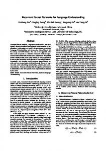
Figure 1: An example RNNLM with an additional input feature vector f . An example RNNLM architecture with an unclustered, full output layer is shown in Figure 1. Without the feature vector f in the input layer, a standard RNNLM is constructed. RNNLMs can be trained using an extended form of the standard back propagation algorithm, back propagation through time (BPTT) [16], where the error is propagated through recurrent connections back for a specific number of time steps, for example, 4 or 5 [2]. This allows RNNLMs to keep information for several time steps in the hidden layer. To reduce the computational cost, a shortlist [17, 18] based output layer vocabulary limited to the most frequent words can be used. To reduce the bias to in-shortlist words during RNNLM training and improve robustness, an additional node is added at the output layer to model the probability mass of out-of-shortlist (OOS) words [19, 20, 21]. RNNLMs can be trained efficiently on GPUs using the spliced sentence bunch technique [22, 23, 24]. Informative features could be incorporated into the training of RNNLMs for adaptation purpose. In Figure 1, feature vector f is appended to the input layer. It will be fed into hidden layer and output layer1 as in [25]. In state-of-the-art ASR systems, RNNLMs are often linearly interpolated with n-gram LMs to obtain both a good context coverage and strong generalisation [1, 3, 17, 18, 19, 20]. The interpolated LM probability is given by P (wi |hi ) = λPNG (wi |hi ) + (1 − λ)PRNN (wi |hi )
(1)
where λ is the weight of the n-gram LM PNG (·), and is kept fixed at 0.5 in this paper. In the above interpolation, the probability mass of OOS words assigned by the RNNLM component is re-distributed with equal probabilities among all OOS words. 1 According
to our experimental results, the direct connection between input (block f ) and output layer is crucial when the hidden layer size is small (e.g. < 50). When the size of hidden layer becomes large (e.g. > 100), there is no difference between using and not using the direct connection. In this paper, the direct connection is used.
3. Feature Based RNNLM Adaptation In this paper, feature based RNNLM adaptation performed at either the show or genre level is studied and compared. As text data often contains a mix of different broad genres, RNNLMs can be refined by making use of the genre information. The first and most straightforward way is to further train or fine-tune a well-trained genre-independent RNNLM on genrespecific data to construct genre-dependent RNNLMs. At test time, for each show, the genre-specific RNNLM is applied according to the show’s genre label. The potential drawbacks of this method are that multiple RNNLMs for each genre needs to be stored and sufficient data for each genre must be obtained for good genre-specific performance. An alternative approach to constructing genre dependent RNNLMs is to incorporate the genre label into the training of the RNNLM. The genre label could simply be represented as a 1-of-k encoding feature vector in the input layer as shown in Figure 1. In many applications, the genre label is not known and could be difficult to estimate. Furthermore, the genre label is normally a coarse representation of the types of topic that might be used. Hence, a more refined representation is preferred to automatically derive a topic representation for each show (i.e. document). This show-level topic representation f , will be concatenated with the standard input layer for RNNLM training and testing as shown in Figure 1.
4. Learning Topic Representations Various topic models have been proposed for topic representation of documents, including probabilistic latent semantic analysis, latent Dirichlet allocation and hierarchical Dirichlet processes. Both PLSA and LDA use a fixed number of latent topics. In contrast, HDP is able to estimate the posterior of the number of topics during training. Let D = {d1 , ..., dN } denote the training corpus, W = {w1 , ..., wM } is all words in the vocabulary, T = {z1 , ..., zK } is the set of latent topics, and n(di , wj ) is the word count wj appearing in document di . For each document di , a vector of posterior probabilities among topics f = {P (z1 |di ), ...P (zk |di ), ...P (zK |di )} is derived from the specˆ T , where each topic has a multinomial disified topic model M tribution over the given vocabulary. When incorporating the feature f into RNNLM training as shown in Figure 1, a Bayesian interpretation of the RNNLM probability for word wi in a document d′ is given by ZZ Prnn (wi |hi , D, d′ ) = Prnn (wi |hi , f )P (f |MT , d′ ) P (MT |D)df dMT
(2)
where P (f |MT , d′ ) is the topic posterior of d′ given a model MT trained on corpus D. The exact computation of the above integral is intractable in general. Hence, approximations are required to make it feasible. For topic model MT , a MAP estimate is instead used ˆ T = arg maxP (MT |D) = arg maxP (D|MT ) M MT
(3)
MT
when a uniform prior P (MT ) is used. When a further approxˆ T , d′ ) ≈ δ(f − fˆ ˆ ′ ), the topic imation is made, P (f |M MT ,d ˆ T ). posterior fˆMˆT ,d′ can be obtained by maximising P (d′ |M Hence, the process in Equation (2) is be simplified as, ˆ T as in Eqn. (3); • maximum likelihood estimation of M
• computing the topic posterior vector fˆMˆT ,d′ for docuˆT ); ment d′ by maximising P (d′ |M • fˆ ˆ ′ is used in RNNLM training or adaptation. MT ,d
4.1. Probabilistic Latent Semantic Analysis PLSA [13, 26, 27] is a generative model defined over a given set of documents. Each of them is generated from a mixture of latent topics. The EM algorithm is applied to maximise the following likelihood criterion, ln P (D|MT ) =
M N X X
n(di , wj ) ln
i=1 j=1
K X
M X
n(d′ , wj ) ln
j=1
K X
P (zk |d′ )P (wj |zk ),
k=1
where P (zk |d′ ) is found as QM n(d′ ,wj ) P (d′ |zk ) j=1 P (wj |zk ) = PK Q M . PK n(d′ ,wj ) ′ m=1 P (d |zm ) m=1 j=1 P (wj |zm )
4.2. Latent Dirichlet Allocation
LDA [14, 28] adds a prior distribution p(θ; α) to relax the constraint of using a fixed set of document level topic posteriors {P (zk |di )} in PLSA. Given a hyper-parameter α, a multinomial parameter distribution p(θ; α) is sampled. The document topic posteriors {P (zk |di )} are then sampled from this distribution. The following likelihood is maximised during training !n(di ,wj ) Z Y N M K X X ln P (D|MT ) = ln P (wj |zk )P (zk |θ) p(θ; α)dθ i=1
j=1
k=1
The exact posterior inference using LDA is intractable, and a variational approximation or a sampling approach can be used instead. The Gibbs Sampling based implementation in [29] is used in this work. The posterior probability of each topic zk given document d′ is computed as n(d′ , zk ) + α ′ m=1 (n(d , zm ) + α)
P (zk |d′ ) = PK
(4)
where n(d′ , zk ) is the number of samples belonging to zk for document d′ . 4.3. Hierarchical Dirichlet Process HDP [15] is a nonparametric Bayesian model for clustering problems with multiple groups of data. Its modelling hierarchy consists of two levels. The first level samples the number of topics and topic-specific parameters. The bottom level samples the topic assignment for each word in each document based on the samples drawn from the top level. In PLSA and LDA, the number of topics is chosen empirically, while HDP can estimate the posterior probability over the number of topics. Eqn. (2) can be rewritten by sampling the topic model MkT with k topics from MkT ∼ P (MT |D) as Prnn (wi |hi , D, d′ ) =
1 NMT
T
ing P (d′ |MkT ). However, directly computing Eqn. (5) is not practical as it requires to train multiple RNNLMs for varying numbers of topics. To address this issue, the MAP estimate ˆ T = arg maxP (D|MkT ) is used as an approximation. The M open-source toolkit2 for HDP based on MCMC sampling is used in this work. The topic posterior probabilities P (zk |d′ ) on test document d′ are computed as in Eqn. (4).
5. Experiments 5.1. Experimental Setup
P (zk |di )P (wj |zk )
k=1
where n(di , wj ) is the count of word wj occurring in document di . For a test document d′ , the topic probability P (zk |d′ ) is obtained by fixing P (wj |zk ) and maximising ˆT ) = ln P (d′ |M
where the topic posterior fˆMk ,d′ can be obtained by maximis-
An archive of multi-genre broadcast television shows were supplied by the British Broadcasting Corporation (BBC) and were used for experiments. A total of seven weeks of BBC broadcasts with original subtitles were made available and this gave after suitable processing and alignment about 1000 hours of acoustic training data. A carefully transcribed test set containing 16.8 hours of data from 40 shows broadcast from one week was used. A baseline acoustic model used standard PLP cepstral and differentials transformed with HLDA and modelled with decision tree clustered cross-word triphones and used MPE training. An improved Tandem model used 26 additional features generated by a deep neural network (DNN) with a bottleneck[30] layer. Both a speaker independent version of this system (Tandem-MPE) and one with CMLLR-based adaptive training (Tandem-SAT) were used. The hypotheses from the TandemMPE model was used as adaptation supervision. Details of the construction of Tandem acoustic models can be found in [32]. The baseline 4-gram (4g) language model was trained on about 1 billion words of text collected for US English broadcast news and the 11 million words (MW) of BBC acoustic model transcription with slight prunning, which includes 145M 3gram and 164M 4gram entries. A 64K word list was used for decoding and language model construction. The RNNLM was trained on the 11MW data using a 46K word input shortlist and 35K output shortlist. The 2231 BBC shows are labelled with 8 different genres (advice, children, comedy, competition, documentary, drama, event and news). Genre advice children comedy competition documentary drama events news Sum
Train #token #show 1.8M 269 1.0M 418 0.5M 154 1.6M 271 1.6M 302 0.8M 149 1.2M 180 3.1M 488 11.5M 2231
Test #token #show 24.4K 3 20.8K 7 27.2K 5 25.8K 6 57.8K 6 20.3K 3 28.7K 5 22.2K 5 227.1K 40
Table 1: Statistics of the BBC training and test data Table 1 gives the statistics of the 11MW BBC data. The average sentence length (with sentence start and end) on the subtitle training set and the test set with manual segmentation are 19.3 and 9.7 respectively and the OOV rate is 1.39%. The corpus is shuffled at the sentence level for RNNLM training. Stop words are removed for training of topic representations.3 . For training of genre dependent RNNLMs, a genre independent
NM
XT
n=1
Prnn (wi |hi , fˆM k(n) ,d′ ), T
(5)
2 http://www.cs.princeton.edu/ 3 Using
chongw/resource.html stop words doesn’t affect performance in our experiments
model is first trained on all 11M data, then followed by finetuning on genre-specific data or the use of a genre input code. To allow the use of show-level topic adaptation, RNNLMs were trained from scratch with the topic representation as an additional input. The RNNLMs had 512 node hidden layer and were trained on a GPU with a 128 bunch size [33]. RNNLMs were used in lattice rescoring with a 4-gram approximation as described in [21]. All word error rate (WER) numbers are obtained using confusion network (CN) decoding [34]. For all results presented in this paper, matched pairs sentence-segment word error (MAPSSWE) based statistical significance test was performed at a significance level of α = 0.05.
Topic M
Sup
-
hyp ref hyp ref hyp ref
PLSA LDA HDP
LM 4g rnnlm +genre.finetune +genre.id
PPL RNN +4g 123.4 152.5 113.5 148.7 110.4 144.2 109.3
WER 32.07 31.38 31.29 31.24
WER 31.38 31.16 31.08 31.14 31.07 31.19 31.10
Table 3: PPL and WER of RNNLMs with topic representation Topic Dim 20 24 30 40
5.2. Results for RNNLMs trained on 11M words Table 2 gives the PPL and WERs for genre dependent RNNLMs. From the results, the use of genre independent RNNLMs gives a significant WER reduction of 0.7% absolute. Genre dependent RNNLMs trained using both fine-tuning and genre-codes both gave small statistically significant WER reductions. The use of a genre-code is preferred since only one RNNLM needs to be trained.
PPL RNN +4g 152.5 113.5 137.8 106.3 137.3 105.1 133.7 105.0 134.1 104.2 138.9 106.6 138.0 105.2
PPL RNN +4g 138.7 106.4 139.3 105.8 134.1 104.2 137.1 104.3
WER 31.13 31.16 31.07 31.11
Table 4: PPL and WER of RNNLM adaptation with LDA using different numbers of topics 5.3. Results for RNNLM trained on 630M words An additional 620MW of BBC subtitle data were also available for LM training. A 4-gram LM trained on the 620M BBC subtitle data was interpolated with the baseline 4g LM trained on 1 billion words. RNNLMs were trained on all 630M of text, consisting of the 620M BBC subtitles and the 11MW of acoustic model transcription. RNNLMs with 512 hidden nodes were again used.
Table 2: PPL and WER of genre dependent RNNLMs In the next experiment, RNNLMs trained with show-level topic representations were evaluated. In [9], each sentence was viewed as a document in the training of LDA, and a marginal (0.1%) performance gain was reported on a system using an MPE-trained acoustic model. In this work, each show is processed as a document for robust topic representation. The testset topic representation is found from the recognition hypotheses using the 4-gram LM after CN decoding. For comparison purposes the reference transcription is also used. For PLSA and LDA, the number of topics used is 30 unless otherwise stated. An initial experiment used the non-Tandem MPE acoustic model. The RNNLM gave 0.7% absolute WER reduction over the 4-gram LM, and the LDA based unsupervised adaptation gave a further 0.4% WER reduction. The experimental results using Tandem-SAT acoustic models are shown in Table 3. PLSA and LDA gives comparable PPL and WER results. A 0.2% to 0.3% WER improvement4 and 8% PPL reduction were achieved. This is consistently better than genredependent RNNLMs. It is worth noting that the PLSA and LDA derived from reference (supervised) and hypotheses (unsupervised) gave comparable performance. This shows that the topic representation inference is quite robust even when the WER is higher than 30%. The number of topics chosen by HDP is 24, giving a slightly poorer PPL and WER than LDA and PLSA. It is maybe related to parameter tuning since the number of topics chosen by HDP was found sensitive to initial parameters. Table 4 gives the PPL and WER results with different numbers of LDA topics derived from the reference. The results show that the performance is fairly insensitive to the number of topics and 30 gives the best performance in terms of PPL and WER. 4 WER
improvements are statistically significant.
LM
PPL
WER
4-gram(1.0G) 4-gram(1.6G) +rnnlm(630M) +rnnlm(630M+LDA)
123.4 103.9 94.4 89.6
32.07 30.84 30.18 30.03
Table 5: PPL and WER of RNNLM trained on 630MW data Table 5 presents the PPL and WER results with the additional 620M words of BBC subtitles. This subtitle corpus reduced the WER by 1.2% absolute using a 4-gram LM, and the RNNLM trained on 630M gives a further 0.7% reduction in WER. RNNLMs with LDA topic features provided an additional 0.15% WER reduction5 and a 5% PPL reduction with unsupervised topic adaptation.
6. Conclusions In this paper, RNNLM adaptation at the genre and show level were compared on a multi-genre broadcast transcription task. Simple fine-tuning on genre specific training data and the use of a genre code as an additional input give comparable performance. A genre code is preferred since it only uses a single model. Continuous vector topic representations such as PLSA, LDA and HDP were incorporated into the training of RNNLMs for show-level adaptation, and consistently outperformed genre level adaptation. Perplexity and moderate WER reductions were achieved on a state-of-art ASR system. Furthermore, the use of LDA based topic adaptation is also effective when RNNLMs are trained on a much larger corpus. 5 WER
reduction is statistically significant.
7. References [1] T. Mikolov, M. Karafi´at, L. Burget, J. Cernock`y, and S. Khudanpur, “Recurrent neural network based language model.” Proc. Interspeech, 2010, pp. 1045–1048. [2] T. Mikolov, S. Kombrink, L. Burget, J. Cernocky, and S. Khudanpur, “Extensions of recurrent neural network language model,” Proc. ICASSP, 2011, pp. 5528–5531. [3] M. Sundermeyer, I. Oparin, J.-L. Gauvain, B. Freiberg, R. Schluter, and H. Ney, “Comparison of feedforward and recurrent neural network language models,” Proc. ICASSP, Vancouver, Canada, May 2013, pp. 8430–8434. [4] K. Yao, G. Zweig, M.-Y. Hwang, Y. Shi, and D. Yu, “Recurrent neural networks for language understanding.” Proc. Interspeech, 2013, pp. 2524–2528. [5] G. Mesnil, X. He, L. Deng, and Y. Bengio, “Investigation of recurrent-neural-network architectures and learning methods for spoken language understanding.” Proc. Interspeech, 2013. [6] C. Chelba, T. Mikolov, M. Schuster, Q. Ge, T. Brants, P. Koehn, and T. Robinson, “One billion word benchmark for measuring progress in statistical language modeling,” Google, Tech. Rep., 2013. [Online]. Available: http://arxiv.org/abs/1312.3005 [7] X. Chen, M. Gales, K. Knill, C. Breslin, L. Chen, K. Chin, and V. Wan, “An initial investigation of long-term adaptation for meeting transcription,” Proc. Interspeech, 2014. [8] Y. Wu, H. Yamamoto, X. Lu, S. Matsuda, C. Hori, and H. Kashioka, “Factored recurrent neural network language model in TED lecture transcription.” Proc. IWSLT, 2012, pp. 222–228. [9] T. Mikolov and G. Zweig, “Context dependent recurrent neural network language model.” Proc. SLT, 2012, pp. 234–239. [10] T.-H. Wen, A. Heidel, H.-Y. Lee, Y. Tsao, and L.-S. Lee, “Recurrent neural network based personalized language modeling by social network crowdsourcing.” Proc. Interspeech, 2013. [11] Y. Shi, “Language models with meta-information,” Ph.D. dissertation, TU Delft, Delft University of Technology, 2014. [12] O. Tilk and T. Alumae, “Multi-domain recurrent neural network language model for medical speech recognition,” in Proc. HLT, vol. 268, 2014. [13] T. Hofmann, “Probabilistic latent semantic indexing,” in Proc. 22nd ACM SIGIR conference, 1999, pp. 50–57. [14] D. M. Blei, A. Y. Ng, and M. I. Jordan, “Latent Dirichlet allocation,” The Journal of Machine Learning Research, vol. 3, pp. 993–1022, 2003. [15] Y. W. Teh, M. I. Jordan, M. J. Beal, and D. M. Blei, “Hierarchical Dirichlet processes,” Journal of the American Statistical Association, vol. 101, no. 476, 2006. [16] D. E. Rumelhart, G. E. Hinton, and R. J. Williams, Learning representations by back-propagating errors. MIT Press, Cambridge, MA, USA, 1988. [17] H. Schwenk, “Continuous space language models,” Computer Speech & Language, vol. 21, no. 3, pp. 492–518, 2007.
[18] A. Emami and L. Mangu, “Empirical study of neural network language models for Arabic speech recognition,” Proc. IEEE Workshop on ASRU, 2007, pp. 147–152. [19] J. Park, X. Liu, M. J. F. Gales, and P. C. Woodland, “Improved neural network based language modelling and adaptation,” Proc. ISCA Interspeech, 2010, pp. 1041– 1044. [20] H.-S. Le, I. Oparin, A. Allauzen, J. Gauvain, and F. Yvon, “Structured output layer neural network language models for speech recognition,” IEEE Transactions on Audio, Speech, and Language Processing, , vol. 21, no. 1, pp. 197–206, 2013. [21] X. Liu, Y. Wang, X. Chen, M. Gales, and P. C. Woodland, “Efficient lattice rescoring using recurrent neural network language models,” Proc. ICASSP, 2014. [22] X. Chen, Y. Wang, X. Liu, M. Gales, and P. Woodland, “Efficient GPU-based training of recurrent neural network language models using spliced sentence bunch,” Proc. Interspeech, 2014. [23] X. Chen, X. Liu, M. Gales, and P. C. Woodland, “Improving the training and evaluation efficiency of recurrent neural network language models,” Proc. ICASSP, 2015. [24] X. Chen, X. Liu, M. Gales, and P. C. Woodland, “Recurrent neural network language model training with noise contrastive estimation for speech recognition,” Proc. ICASSP, 2015. [25] T. Mikolov and G. Zweig, “Context dependent recurrent neural network language model.” Proc. SLT, 2012, pp. 234–239. [26] D. Mrva and P. C. Woodland, “A PLSA-based language model for conversational telephone speech.” Proc. Interspeech, 2004. [27] D. Gildea and T. Hofmann, “Topic-based language models using EM.” Proc. Eurospeech, 1999. [28] Y. C. Tam and T. Schultz, “Unsupervised language model adaptation using latent semantic marginals.” Proc. Interspeech, 2006. [29] X.-H. Phan and C.-T. Nguyen, “GibbsLDA++: A C/C++ implementation of latent Dirichlet allocation (LDA),” 2007. [30] F. Grezl and P. Fousek, “Optimizing bottle-neck features for LVCSR,” Proc. ICASSP, 2008, pp. 4729–4732. [31] J. Park, F. Diehl, M. J. F. Gales, M. Tomalin, and P. C. Woodland, “The efficient incorporation of MLP features into automatic speech recognition systems,” Computer Speech & Language, vol. 25, no. 3, pp. 519–534, 2011. [32] P. Lanchantin, P. J. Bell, M. J. Gales, T. Hain, X. Liu, Y. Long, J. Quinnell, S. Renals, O. Saz, M. S. Seigel, P. C. Woodland, “Automatic transcription of multi-genre media archives,” Proc. First Workshop on Speech, Language and Audio in Multimedia, 2013. [33] X. Chen, Y. Wang, X. Liu, M. Gales, and P. C. Woodland, “Efficient training of recurrent neural network language models using spliced sentence bunch,” Proc. Interspeech, 2014. [34] L. Mangu, E. Brill, and A. Stolcke, “Finding consensus in speech recognition: word error minimization and other applications of confusion networks,” Computer Speech & Language, vol. 14, no. 4, pp. 373–400, 2000.