Model-Based Recurrent Neural Network for Fault Diagnosis of

CHAPTER 7 Model-Based Recurrent Neural Network for Fault Diagnosis of Nonlinear Dynamic Systems C. Gan and K. Danai Department of Mechanical and Industrial Engineering University of Massachusetts Amherst, Massachusetts U.S.A. A model-based recurrent neural network (MBRNN) is presented for modeling dynamic systems and their fault diagnosis. This network has a fixed structure that is defined according to the linearized state-space model of the plant. Therefore, the MBRNN has the ability to incorporate the analytical knowledge of the plant in its formulation. Leaving the original topology intact, the MBRNN can subsequently be trained to represent the plant nonlinearities through modifying its nodes’ activation functions, which consist of contours of Gaussian radial basis functions (RBFs). Training in MBRNN involves adjusting the weights of the RBFs so as to modify the contours representing the activation functions. The performance of the MBRNN is demonstrated via several examples, and in application to the IFAC Benchmark Problem. The results indicate that MBRNN requires much shorter training than needed by ordinary recurrent networks. This efficiency in training is attributed to the MBRNN’s fixed topology which is independent of training. In application to fault diagnosis, a salient feature of MBRNN is that it can be formulated according to the present model-based fault diagnostic solutions as its starting point, and subsequently improve these solutions via training by adapting them to plant nonlinearities. The diagnostic results indicate that the MBRNN performs better than ‘black box’ neural networks.

2

1

C. Gan and K. Danai

Introduction

The need for modeling complex industrial systems demands modeling methods that can cope with high dimensionality, nonlinearity, and uncertainty. As such, alternatives to traditional linear and nonlinear modeling methods are needed. One such alternative is neural network modeling. Artificial neural networks are powerful empirical modeling tools that can be trained to represent complex multi-input multi-output nonlinear systems. Neural networks are also pattern classifiers, so they provide robustness to parameter variations and noise. Various types of neural networks have been used for modeling dynamic systems. Multi-layer perceptrons have been used to provide an inputoutput representation of the plant in auto-regressive moving average (ARMA) form for cases where the past values of the plant inputs and outputs are available as network inputs [1]. Another network used for modeling dynamic systems is the cerebellar model articulation controller (CMAC) [2], noted for its ability to represent the spacial aspects of the system and for its fast learning that is desired for on-line applications [3]. Multilayer perceptrons and CMAC networks, however, are feedforward networks that only provide static mapping between inputs and outputs. A more suitable network for representing dynamic systems is the recurrent network which has the inherent format to internally represent the autoregressive aspect of dynamic systems [4], [5], [6], [7]. Regardless of their type, however, neural networks are generally disadvantaged by their ‘black box’ format. They need training for defining their structure (number of nodes) as well as their connection weights [7]. Therefore, these networks require prohibitively extensive training, and are hard to interpret once trained. One variant to these networks is the diagonal recurrent neural network proposed by Ku and Lee [8] that provides a simpler structure than the fully connected network, and therefore is an easier network to train. Another variant is a simplified network that is initiated based on representative patterns in the training data [9]. While the above solutions have led to reduced demand for training, they have not been significant, mostly due to their reliance on empiricism. Ideally, neural networks should be less empirical, to reduce the demand

Model-Based Recurrent Neural Network for Fault Diagnosis

3

for training, and more transparent, to provide insight into their representation. A step toward such an ideal solution for modeling dynamic systems is using sub-networks to represent separately the autoregressive and moving average parts of the plant, and selecting the complexity of these networks according to linearity/nonlinearity of these parts [10]. Although this modular solution takes advantage of the existing knowledge of the plant to reduce the complexity of the overall network and, consequently, reduces the demand for training, it does not contribute to improving the transparency of the network, as it still uses a black box format for the individual sub-networks. Perhaps a more fundamental step towards the ideal solution has been in the area of neuro-fuzzy inference systems [11], [12] and knowledgebased artificial neural networks (KBANN) [13], [14]. In the neuro-fuzzy approach, the heuristic knowledge of the process is expressed in the form of rules between inputs and outputs, and incorporated in a feedforward network with several layers, where each layer performs a step of inference. An important feature of neuro-fuzzy networks is their equivalence to Gaussian radial basis function (RBF) networks [11], which makes possible the use of learning algorithms associated with RBF networks to modify the rules. Knowledge-based artificial neural networks (KBANN) are formulated by symbolic rules in the form of propositional logic [13]. Both the neuro-fuzzy system and KBANN provide methods for incorporating the existing knowledge of the plant in a neural network. However, they require that this knowledge be formulated as heuristics or propositional logic. Given that most plant models are developed from first principles and are in analytical form, these methods would either ignore the existing analytical models or require the extra step of converting these models into heuristics or propositional logic. The objective of this chapter is to introduce a method of incorporating the analytical knowledge of the plant in a recurrent neural network. This model-based recurrent neural network (MBRNN) will be formulated according to a linearized state-space model of the dynamic system. It will then be trained to adapt its activation functions to the nonlinearities of the plant as reflected in the training data. As such, the topology of the MBRNN will remain intact, and adaptation to nonlinearities will be confined to the activation functions of individual nodes. The activation

4

C. Gan and K. Danai

functions in MBRNN are defined as contours of the RBFs that comprise the node, therefore, adaptation entails changing the weight of individual RBFs within each node.

2

Methodology

The model-based recurrent neural network (MBRNN) is structured according to a linearized state-space model of the plant. It, therefore, assumes that an analytical model of the plant is available which can be linearized about an operating point. If the discrete-time nonlinear statespace model of the plant is defined as:

x(k + 1) = [x(k); u(k)]

(1)

y(k) = [x(k); u(k)]

(2)

x(k + 1) = Ax(k) + Bu(k)

(3)

y(k) = Cx(k) + Du(k)

(4)

() ()

()

where u k , x k , and y k represent the sampled values of the inputs, states, and outputs at time k , respectively, then the linearized state-space model has the form:

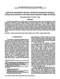
The above model can be formulated as a recurrent neural network, having the same number of inputs and outputs. An example of such a network is shown in Figure 1 for the second-order model: "

x1 (k + 1) x2 (k + 1) "

y1 (k) y2 (k)

#

#

=

= "

"

a11 a12 a21 a22

c11 c12 c21 c22

#"

#"

x1 (k) x2 (k)

x1 (k) x2 (k)

#

#

+

+ "

"

d1 d2

b1 b2 #

#

u(k)

u(k)

(5)

(6)

Note that the nodes of this initial MBRNN have a gain of 1 (i.e., their output equals their input) to initially represent the linearized model (see Figure 1), but the activation functions of these nodes are subsequently adapted during training into nonlinear functions so as to represent the

Model-Based Recurrent Neural Network for Fault Diagnosis

5

z -1 c 11

a11 a 12

x1

b1

c 12 d1

b2 a 21

d2 c 21

x1

y1

u x2

x2

a 22

y2

c22

z -1 Figure 1. A model-based recurrent neural network (MBRNN) representing a second-order plant.

plant nonlinearity. As such, adaptation in MBRNN is performed by only changing the form of the activation functions, leaving the connection weights intact. In order to provide adaptability, the activation functions in MBRNN are defined as contours of radial basis functions that comprise the node. If the output of each RBF is defined as o jx c j2=2 (7) i

= exp(

j

i

)

to represent a normal distribution with localized characteristics, then the activation function of the node will have the form,

Oj

=

N X i=1

i oi =

N X i=1

i exp( jxj

ci j2 = 2 )

(8)

While the activation function Oj can be composed of an array of any basis function that can be adapted on-line, it is desirable that the basis function should have a localized characteristic so that the activation function can be modified locally without affecting the value of the function at neighboring points. The above formulation represents a modular format for MBRNN where each module consists of an RBF network denoting a node. Training consists of adjusting the weights i of individual RBFs to shape the node’s

6

C. Gan and K. Danai

activation function. The above second-order network with an adaptable set of activation functions has the form: (

x1 (k + 1) x2 (k + 1)

)

"

=

a11 a21

"

a12 a22

"

"

y1 (k ) y2 (k )

#

"

=

b1

c11 c12 c22

"

11  a11 exp( i  a21 exp(

i=1 PNa 21 i=1 PNa

PNb

PNc

i

12  a12 exp( i  a22 exp(

i=1 PNa 22 i=1

i

1  b1 exp( i  b2 exp(

i=1 PNb b2 i=12

c21 "

PNa

i

11  c11 exp( i  c21 exp(

i=1 PNc 21 i=1

i

PNc

12 c12 i=1 i exp( PNc 22  c22 exp( i=1

PNd

i

1 d1 i=1 i exp( PNd d2 i=12 id2 exp( d1

jx1 (k) jx1 (k)

cai 11 ca21

#

i

j2 =2 ) j2 =2 )

jx2 (k) jx2 (k)

cai 12 ca22

j2=2 ) j2=2 )

#

ju(k) ju(k) jx1(k) jx1(k) jx2 (k) jx2 (k)

ju(k) ju(k)

i

+

+

#

j2 =2 ) 2 2 i j = ) cci 11 j2 = 2 ) cci 21 j2 = 2 ) cci 12 j2 = 2 ) cci 22 j2 = 2 ) cdi 1 j2 = 2 ) cdi 2 j2 = 2 ) cbi 1 cb2

(9) #

+ #

+

#

(10)

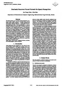
The RBFs in each node of MBRNN are evenly distributed across the expected range of state or input space. For the initial MBRNN, the values of parameters i are selected to produce linear activation functions as their contours, so as to depict the linearized model of the plant. Subsequently, these parameters are modified during a training phase to adapt the MBRNN to plant nonlinearities. Note that MBRNN is formulated such that the activation functions are linear in terms of parameters i , so training is tractable. Based on Eqs. (9) and (10), if the states are measurable, then training of the parameters associated with each of the states and inputs can be carried out separately by the least-squares method. In cases where the states are not accessible, as is often the case, alternative forms of training such as dynamic backpropagation or extended Kalman filtering can be used. In either case, after training the activation functions may have forms very different from their initial linear form, as shown in Figure 2 for a hypothetical case. The construction of the MBRNN’s nodes by normally distributed RBFs provides it with the distinct characteristic of “spacial localization” [15]. Because of one-to-one relationship

Model-Based Recurrent Neural Network for Fault Diagnosis

RBFs

RBFs (a)

7

(b)

Figure 2. An initial linear activation function of MBRNN formed from the contour of RBFs in the node (a), and the trained activation function obtained by modifying the weights of various RBFs (b).

between input-output pairs, each adaptation iteration in MBRNN is confined to a limited number of i that are associated with the excitation input. This, in addition to providing efficient training, enables MBRNN to accommodate localized nonlinearities within limited ranges of the input space. In its present form, the initial MBRNN represents the first-order approximation of the nonlinear plant, and it maintains this first-order representation while allowing the individual components of the linearized model to incorporate nonlinearity through training. As such, this format does not allow inclusion of bilinear terms. For example, if the actual x1 in our example of Eqs. (5) and (6) had the form x1 k F x1 k ; x2 k , and was then approximated by a Taylor Series Expansion, as

( + 1) = ( ( ) ( ))

F (x1 ; x2 ) = F (x1 ; x2 )j0 + 1

@F @x1 @x12

(x1; x2 )(x1

x1 j0 )r (x2

x2 j0 )1

r

+ :::

+ (nr) @x@r @xFn r (x1; x2 )(x1

x1 j0 )r (x2

x2 j0 )n

r

+ :::

X 

r =0

1 r

r

n X

n

1

r =0

( )=

r

2

n! where nr denote the binomial coefficients and all the derivar !(n r )! tives are evaluated at x1 ; x2 j0 , then the MBRNN constructed according to the first-order approximation of function F , would exclude the P n coupling between x1 and x2 , represented by nr=1 nr @xr@@xFn r x1 ; x2 . 1 2

(

)

()

(

)

8

C. Gan and K. Danai

x1

n

x2

m

a n,m

Figure 3. A possible modification to MBRNN to accommodate coupling between x1 and x2 . The nodes with circular arrows pointing to themselves represent the repetitive multiplication of the input variable, i.e., the node with x1 as input to the node enclosing n would output xn1 , and the node with a dot inside signifies the product of the input variables.

Therefore, when this coupling is not negligible, MBRNN, in its present form, will not be able to approximate the nonlinear plant satisfactorily. In order to include such significant coupling terms, additional nodes may be added into the feedforward path of MBRNN to represent specific couplings. One stand-alone node that can represent a coupling term is shown in Figure 3, where the nodes with circular arrows pointing to themselves represent the repetitive multiplication of the input variable (e.g., the node with x1 as input to the node enclosing n would output xn1 ), and the node with a dot inside signifies the product of the input variables. Although the inclusion of such coupling terms in MBRNN is straightforward, it poses two constraints: (1) it requires a knowledge of the dominant coupling between the plant variables, and (2) it adds to the complexity of MBRNN and its demand for learning. A central issue in MBRNN is the number of RBFs needed within each node. Initially, the activation functions should be linear with slopes of 1 so as to provide a uniform gain of unity at all inputs for an accurate representation of x y . A perfect linear activation function, however, would require a large number of RBFs. Therefore, a method needs to be devised to limit the number of RBFs within the expected ranges of inputs and states. One method for selecting the number of RBFs is cross validation, where the available input-output data is divided into two parts, one part used for training and the other for testing. The selection criterion

=

Model-Based Recurrent Neural Network for Fault Diagnosis

9

in this case is the generalization ability of the network based on the test set [16], [17]. For each modular RBF network representing a node, the average of mean-square-error over the training set can be defined as [18]:

2 ^GCV j

^

py^ jT P2j y^ j = trace (P )2

(11)

j

2 where GCV represents the generalized cross-validation (GCV), p dej notes the number of patterns used in training, Pj represents the square matrix which projects p-dimensional vectors onto the mj -basis subspace spanned by the RBFs within the node, and yj denotes the output of the node. Since each node in MBRNN can be perceived as a separate RBF network, GCV can be used to determine the number of RBFs within each MBRNN node. For this, each set of outputs from the p patterns corresponding to each node is projected to the mj -dimension spanned by the RBFs within that node, so as to represent its optimal representation in least-squares sense. The projection matrix Pj for MBRNN is defined as:

^

Pj = Ip Oj Aj 1OTj

(12)

where Oj represents the matrix of RBFs oi for each node (see Eq. (7)) 2

Oj =

6 6 6 6 4

o1 (s1 ) o2 (s1 ) o1 (s2 ) o2 (s2 )









omj (s1 ) omj (s2 )

o1 (sp ) o2 (sp )

.

omj (sp )

.. .

.. .

..






.. .

3 7 7 7 7 5

where si represents the input value associated with pattern i, and denotes the variance matrix of Oj obtained as

Aj 1 = (OTj Oj + j Ip )

1

(13)

Aj 1 (14)

In the above equation, j denotes the regularization parameter associated with each node. Regularization parameters are integral parts of training the activation functions by dynamic backpropagation, so they are included in the formulation of GCV to define the rationale for their selection. Generalized cross-validation is a measure of the network’s ability in mapping a set of inputs to a desired set of outputs. As such, GCV can be used

10

C. Gan and K. Danai 0.9

0.36

0.8

0.34

0.7

0.32 0.3

0.5 0.4

GCV

GCV

0.6

0.3

0.28 0.26

0.2

0.24

0.1 0 20 25 30 35 40 45 50 55 60 65

0.22

No. of RBFs (a)

0.2

0

0.1

0.2

0.3

0.4

Regularization Parameter (b)

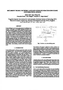
Figure 4. Effect of the number of RBFs (a) and the regularization parameter (b) on the generalized cross-validation (GCV) value.

to determine the value of the regularization parameter and the number of RBFs for each node to provide an accurate representation of y x initially. The typical values of GCV obtained for different numbers of RBFs, with a constant regularization parameter, are shown in Figure 4(a). The results indicate that the increasing number of RBFs has a diminishing effect on the GCV value, so the GCV value can be used as the basis of selecting the RBF numbers. Similarly, the effect of the regularization parameter on the GCV value of the node, with a fixed number of RBFs, is shown in Figure 4(b). The results indicate that the accuracy of each node’s output (as represented by the GCV value) is directly affected by the regularization parameter, and that an ‘optimal’ value for it can be selected based on the GCV value. Of course, one should note that there is a correlation between the number of RBFs and the value of regularization parameter, and that by determining each independent of the other there is no assurance that their optimal values have been selected. Experience, however, indicates that selecting the number of RBFs and the regularization parameter separately leads to satisfactory results.

=

3

Training

An important feature of MBRNN is the linearity of its activation functions in terms of the RBF weights, which makes possible adapting the RBF weights by various linear regression methods. An important objec-

Model-Based Recurrent Neural Network for Fault Diagnosis

11

tive of MBRNN design is to adhere to its initial format which is structured according to the state-space model of the plant. In order to satisfy this objective, limited changes should be made to the shape of the activation functions during training, so as to (1) avoid drastic deviations from the initial structure of MBRNN, and (2) avoid creation of limit cycles. Two adaptation methods that can implement such a restriction, based on dynamic backpropagation [19], [20] and extended Kalman filter (EKF) [21], [15], [7] are described here, to estimate the network parameters  and  in the MBRNN representation of the nonlinear plant, as xk net x k ; u k ;  (15)

^ ( + 1) = [^ ( ) ( ) ] y^ (k) = net [^x(k); u(k);  ] where x 2 Rn , u 2 Rm , and y 2 Rq .

3.1

(16)

Training by Dynamic Backpropagation

For the p input-output training pairs, the objective function can be defined as: p X J yi yi 2 (17) i=1 where y denotes the vector of network outputs and y the corresponding plant outputs. Although this objective function is suitable for adaptation of the network parameters, it does not satisfy the goal of preserving its structure. This restriction on the extent of parameter changes can be imposed by including a regularization term in the objective function, as

= (^

)

^

J

X

p

N X

j =1

j =1

= (^yj yj )2 +

j

m

j X i=1

(i

i0 )2

(18)

where N denotes the number of nodes in MBRNN, mj represents the number of RBFs in individual nodes, i denotes the weight of each RBF during training, i0 represents the initial weight of each RBF, and j denotes the regularization parameter of each node (see Eq. (14)). MBRNN consists of two parts (see Figure 1): a recurrent part, which emulates the state equations (Eq. (1)), and a feedforward part, that represents the output equations (Eq. (2)). Training of the recurrent part can

12

C. Gan and K. Danai

be performed by backpropagation (BP) over time (dynamic BP), to estimate  , whereas the the static part can be trained by regular BP, to estimate  . The objective of training is to determine the vector   which minimizes the objective function J in Eq. (18) by moving the parameter vector along the negative gradient of the objective function with respect to  , as [22] k  k  r J k (19)

( + 1) = ( ) () where  denotes the learning rate, r J represents the gradient of the objective function, and  (k ) represents the current value of the RBFs

weight vector.

For the dynamic part of MBRNN, the change in a weight at time k will result in a change in the output y t for all t  k . This means that the present value of the output y t is not only affected by the current value of the weight vector  k , for k t, but by all the past values of  k , for  k  t, as well. This implies that weight adaptation should be performed with regard to past adaptations, as reflected in the estimate of the gradient of the objective function, computed from Eqs. (15) and (16):

^( ) ^( ) () =

0

@ x^ (k + 1) @ (k)

@ y^ (k) @ (k)

= @ net (^x(k@)x^; (uk()k); (k)) @@ x^ ((kk)) +  @ net (^x(k); u(k);  (k)) @ (k) = @ net (^x(k@)x^;(uk()k);  (k)) @@ x^ ((kk)) +  @ net (^x(k); u(k);  (k)) @ (k)

()

(20)

(21)

The components of the above equations can be computed at each instant k to yield @ y=@ as the gradient of the objective function with respect to the RBF weights. Dynamic BP can then be used to adapt the parameter vector  according to the learning rule in Eq. (19). Note that Eqs. (20) and (21) define a state-space representation of the gradient of the objective function r J used in Eq. (19). The drawback of backpropogation is that it is often too slow for practical application. There are many variations on backpropogation that speed up the training, such

^

Model-Based Recurrent Neural Network for Fault Diagnosis

13

as the Levenberg-Marquardt algorithm, BP with Momentum, etc. [23]. Also, in order to eliminate the spikes during training, a low-pass filter can be incorporated in training. Another issue in training by backpropagation is the proper choice of the learning rate  (see Eq. (19)). Usually small values of  guarantee convergence, but at a very low speed. Larger values of  , on the other hand, may lead to instability. It is possible to determine analytically the range of  to guarantee stability.

3.2

Training by the Extended Kalman Filter

The MBRNN can also be trained by the Extended Kalman Filter (EKF) [15], [7], which has the added appeal of being applicable to both the recurrent and feedforward parts of the network. EKF-based training is also faster than dynamic BP, and is less prone to noise. In application to MBRNN, the network states are augmented with auxiliary states that correspond to the RBF weights. As such, EKF-based training of MBRNN consists of simultaneous parameter and state estimation. Since the network inputs lie in < > :

x1 (k + 1) x2 (k + 1) x3 (k + 1)

2 6 4

9 > = > ;

=

0:3(x1 (k) + sin2 (x1(k))) 0 0 u 2:9x1 (k) 0:62x2 (k) 2:3x3 (k) + 0 0 2:3x2 (k) 0 0 (35) x1 (k) 1 1 0 x2 (k) + 0 u y (k) = (36) 1 3 1 x3 (k) 1 3 7 5

"

8 #>
=

> :

> ;

"

8 >
=

> :

> ;

#

The above model represents a single-input multiple-output system, with nonlinear state equations. The linearized state-space model of this plant about the operating point x1 ; x2 ; x3 was obtained as: 8 > < > :

x1 (k + 1) x2 (k + 1) x3 (k + 1)

9 > = > ;

2

=

y (k) =

6 4

"

( =0 0:3 0 2:9 0:62 0 2:3

1 1 0 1 3 1

= 0 = 0) 0 x1 (k ) 1 2:3 x2 (k) + 0 0 x3 (k ) 0 x1 (k) 0 u x2 (k) + 1 x3 (k) 38 > < 7 5 > :

8 #>
=

> :

> ;

"

9 > =

8 >
=

> ;

> :

> ;

u

(37)

#

(38)

C. Gan and K. Danai 1

1

0.5

0.5

0.0

0.0

Outputs

Outputs

18

-0.5 -1.0 -1.5 0

100

200

300

400

500

600

-0.5 -1.0 -1.5 0

100

No. of Samples (a)

200

300

400

500

600

No. of Samples (b)

Figure 6. Outputs of the plant and MBRNN before training (a) and after training by dynamic BP without a regularization parameter (b) for Example 2. 2 1.5 1

Output

0.5 0 -0.5 -1 -1.5 -2

0

5

10

15

20

25

30

35

40

RBF No.

Figure 7. The modified activation function of the a22 component causing the limit cycle problem.

The MBRNN was structured according to the above state-space model and then trained by dynamic BP without a regularization parameter. The training session consisted of 1500 sample points generated with random excitation inputs with values between -6.0 and 6.0. One epoch of training was used. The trained MBRNN was then tested on data generated with random inputs from a seed different from that which generated the training data. The values of y1 and y1 for the test session before and after training are shown in Figure 6. The results indicate a potential pitfall associated with dynamic BP as applied to MBRNN. The reason for the

^

Model-Based Recurrent Neural Network for Fault Diagnosis

19

0.2 0

Outputs

-0.2 -0.4 -0.6 -0.8 -1

0

100

200

300

400

500

600

No. of Samples Figure 8. Output 1 of the plant and MBRNN after training by the extended Kalman filter for Example 2.

poor results in this application is entrapment of the system in a limit cy1 cle at x1 : x2 : x3 : , which is caused by the shape of the activation function shown for one of the nodes in Figure 7. Similar results to those in Figure 6(b) can be obtained by introducing small excitation values for u to net x ; u .

= 0 475 = 0 003 = 0 0751 (

)

The MBRNN was next trained by EKF using the same training data. The values of y1 and y1 from this MBRNN are shown in Figure 8, indicating a much better representation by MBRNN.

^

Example 3: 

2 (m1 + m2 )a2 1 + m2 a2 + 2m2 a1 a2 cos 2 m2 a22 + m2 a1 a2 cos 2

+

"

m2 a22 + m2 a1 a2 cos 2 m2 a22

m2 a1 a2 (2_1 _2 + _22 ) sin 2 m2 a1 a2 _12 sin 2

#

x

1 2



+

+

2) ga1 cos 1 + m2 ga2 cos(1 + 2 ) = + (mm21ga+2 m cos(1 + 2 ) "



#

 x

"

1 2

#

(39)

These points which are the equilibrium points of  = net (  0), represent the coordinates of a stable limit cycle. The stability of this limit cycle is verified by the eigenvalues of the Jacobian being inside the unit cycle. 1

20

C. Gan and K. Danai

The above model represents the dynamics of a two-link plannar elbow robot arm [24], where 1 and 2 represent the angular positions of the two arms, m1 and m2 denote their masses, and 1 and 2 represent the torques exerted on the arms. If we define the position vector q as q 1 2 T and the generalized force vector  as  1 2 T , then the above state-space equation can be written as

=[

=[

]

]

M (q)q + V (q; q_ ) + G(q) = 

()

(40)

( _)

where M q denotes the inertia matrix, V q; q represents the Coriolis/centripetal vector, and G q denotes the gravity vector.

()

The linear state-space form of the above model about T was obtained as

[0 0]

8 > > > < > > > :

x1 (k + 1) x2 (k + 1) x3 (k + 1) x4 (k + 1)

8 > > > < > > > :

y1 (k) y2 (k) y3 (k) y4 (k)

= [ _]

9 > > > = > > > ;

9 > > > = > > > ;

1:0 0:0 0:01 0:0 = 00::00 10::00 01::00 00::01 0 0:0 0:0 0:0 1:0 0:0001 0:0002 0:0002 0:0004 + 0:02 0:04 0:04 0:085 1:0 0:0 0:0 0:0 = 00::00 10::00 01::00 00::00 0:0 0:0 0:0 1:0 2 6 6 6 4

2 6 6 6 4

q = [0 0]T , q_ =

38 > > 7> < 7 7 5> > > :

2

3

6 6 6 4

7 7 7 5

38 > > 7> < 7 7 5> > > :

(

x1 (k) x2 (k) x3 (k) x4 (k) 1 2

x1 (k) x2 (k) x3 (k) x4 (k)

9 > > > = > > > ;

)

9 > > > = > > > ;

where xT q q . The MBRNN was structured according to the above state-space model and then trained by EKF. The training session consisted of 5500 sample points generated by random excitation inputs with values between -1.0 through 1.0 and -0.5 through 0.5 for two inputs, respectively. One epoch of training was used. The trained MBRNN was then tested on data generated with random inputs from a seed different from that which generated the training data. The values of y and y before and after training are shown in Figs. 9 and 10, respectively. The results indicate that the outputs of the trained MBRNN are quite close to the plant outputs, again despite the relatively short training session used by MBRNN.

^

0.4 0.3 0.2 0.1 0.0 -0.1 -0.2 -0.3 -0.4 -0.5 0

State 2

State 1

Model-Based Recurrent Neural Network for Fault Diagnosis

2

4

6

8

10

12

14

0.6 0.4 0.2 0.0 -0.2 -0.4 -0.6 -0.8 -1.0 -1.2 -1.4 0

2

4

0.4 0.3 0.2 0.1 0.0 -0.1 -0.2 -0.3 -0.4 0

6

8

10

12

14

12

14

Time (sec) 0.8

State 4

State 3

Time (sec)

21

2

4

6 8 10 Time (sec)

12

14

0.6 0.4 0.2 0.0 -0.2 -0.4 -0.6 -0.8 -1.0

0

2

4

6 8 10 Time (sec)

0.4 0.3 0.2 0.1 0.0 -0.1 -0.2 -0.3 -0.4 -0.5 0

State 2

State 1

Figure 9. Four states of the plant and MBRNN before training for Example 3.

2

4

6

8

10

12

14

0.6 0.4 0.2 0.0 -0.2 -0.4 -0.6 -0.8 -1.0 -1.2 -1.4

0

2

4

0.4 0.3 0.2 0.1 0.0 -0.1 -0.2 -0.3 -0.4

6

8

10

12

14

12

14

Time (sec) 0.8

State 4

State 3

Time (sec)

0

2

4

6 8 10 Time (sec)

12

14

0.6 0.4 0.2 0.0 -0.2 -0.4 -0.6 -0.8 -1.0 0

2

4

6 8 10 Time (sec)

Figure 10. Four states of the plant and MBRNN after training for Example 3.

22

5

C. Gan and K. Danai

Application in Fault Diagnosis

Fault diagnosis is important for safety-critical and intelligent control systems. The correct detection or prediction of faults will avoid system shutdowns or catastrophes which may involve human lives and material damage. Fault Detection and Isolation (FDI) solutions have been developed within various disciplines. For systems with analytical models, Model-Based FDI offers a system theoretic approach, where the model is used to obtain residuals which represent the difference between the measurements and their modeled values [25]. For cases where the residuals do not provide an adequate basis for fault diagnosis, Statistical FDI can be used to complement the analysis [26]. In a more abstract framework, KnowledgeBased FDI methods rely on the causal knowledge of the system when complexity precludes analytical modeling [27]. In contrast to the above approaches, Neural Network-Based FDI mostly ignores the knowledge of the process and provides an empirical solution by defining the fault signatures based on measurement-fault data. Although neural networks have been developed that can incorporate the knowledge of the process in their formulation [28], they are mostly used in a ‘black box’ format and rely solely on training to define the fault signatures [29]. The utility of the MBRNN is demonstrated in application to the IFAC Benchmark Problem [30]. This benchmark problem represents the nonlinear model of an electro-mechanical position governor used in speed control of large diesel engines. The governor consists of a brushless DC motor that connects to a rod through an epicyclic gear and arm. Two faults are considered (simulated) for this value: (1) a position sensor fault, and (2) an actuator fault. The main source of uncertainty is the load torque, which represents an unknown input.

5.1

The Benchmark Problem

The industrial actuator benchmark was based on a test facility built by the researchers at Aalborg University [30]. The equipment simulates the actuator part of a speed governor for large diesel engines. The governor is a device that controls the shaft rotational speed in a diesel engine. It

Model-Based Recurrent Neural Network for Fault Diagnosis

23

regulates the amount of fuel loaded into each cylinder by controlling the position of a common control rod - equivalent to the throttle in an automobile. The rod can be moved by an actuator motor, which is part of the governor. The current and velocity of the motor are controlled by a power drive made in analog and transistor switch mode technology. The position of the rod is controlled by a micro-processor based digital controller. The system is thus a combination of continuous and discrete-time components. A nonlinear model of this actuator has been made available TM in format, and its linear model, which is the basis for the model-based solutions, is defined as:

Simulink

x(k + 1) y (k )

= x(k) + u(k) + E1ud (k) + F1 fa (k) = Cx(k) + E2ud(k) + F2fs (k) 0:51 0:36 0 0:63 9:09  10 2 0 = 5:41  10 5 3:94  10 5 1 0:38 1:06 = 7:06  10 5 0:49 0 1 0 0:63 F1 = ; C= 0 0 0:98 5:41  10 5 F2 = 0:098 2

3

6 4

7 5

2

3

6 4

7 5

2

3

6 4

7 5

"

"

#

#

where ud represents the unknown torque disturbance, fa denotes the actuator fault, and fs represents the sensor fault. Two possible faults can be simulated for the industrial actuator: 1. A temporary feedback element fault caused by loss of contact of the feedback wiper due to wear and dust. The fault is intermittent, and lasts for 0.2 seconds. 2. A component fault caused by malfunctioning of the end-stop switch. This can be caused by a broken wire or a defect in the switch element due to mechanical vibration, resulting in the power drive delivering only positive current.

24

C. Gan and K. Danai

Both of the above faults are multiplicative in nature, but they are represented as additive faults because most FDI methods are suitable for additive faults. The particular difficulty in FDI of the benchmark is that the load torque acts as an unknown disturbance input signal, which has a similar effect as the actuator fault. This can be noted from the coefficient 2; :  2; :  6 of the disturbance vector E :  d being approximately linearly aligned with the fault weighting vector 5 of the actuator fault fa . That is, the Fa : ; : ; :  angle between these two vectors is so small that it is very difficult to differentiate between the disturbance and actuator fault.

= [ 1 21 10 1 55 10 = [ 0 493 0 635 5 42 10 ]

1 33 10 ]

Briefly, as a solution to this problem, Bogh [31] used model-based and statistical FDI to design a bank of observers to differentiate between faults and unknown inputs through multiple-hypothesis testing. It was shown that statistical testing was needed to improve the detectability of faults. In a similar approach, Grainger et al. [32] proposed a set of sequential probability ratio tests of the innovations from a bank of Kalman filters to detect the change in the dynamics of the system. Hofling and coworkers [33] treated the detection of sensor fault and actuator fault separately. They designed a simple observer-based residual generator with adaptive threshold to detect the sensor fault, and used signal-processing to detect the actuator fault. In a frequency domain approach, Garcia et al. [34] used 1 -based optimization to design observers with residuals that are robust to unknown inputs (noises) and sensitive to the faults. Using the Extended Kalman Filter (EKF) as a parameter estimator, Walker and Huang [35] proposed to detect the faults through estimation of the position sensor bias and the actuator bias. This work showed that the EKF, designed according to a linear model, could detect the fault accurately when the system was excited by small inputs, but the magnitude of the sensor fault residuals were affected by the actuator fault for large inputs. Eigen-Structure Assignment (ESA) was also used to design residual generator observers that produced residuals de-coupled from disturbance inputs [36]. This method was successful in detecting faults in presence of small inputs and disturbances, but it was unable to detect the actuator fault for large input signals.

H

Model-Based Recurrent Neural Network for Fault Diagnosis

5.2

25

Traditional Neural Network Application

An overview of neural networks (NNs) FDI application of is presented in [29]. In most applications, the NNs have a black box format, so they require for training measurement data from normal operation of the plant as well as during fault occurrences. For example, a dynamic plant described by the nonlinear ARMA model:

y (k )

=

F (y(k

1);

y (k

2);




; y (k

ny );

u(k); u(k 1);


; u(k nu); d(k);


; d(k nd ); f (k);


; f (k

nf ))

can be modeled by a recurrent NN using as inputs the present values of the plant inputs and outputs to generate as output an estimate of the fault. In the above model, d represents disturbance to the plant, and f denotes the sensor fault, actuator fault, or component fault. Using recurrent NNs, one scenario for residual generation is as shown in Figure 11, where the NN provides a nonlinear mapping from the measurement space Y; U to fault space F . The nonlinear mapping demand from the NN can be relaxed in cases where a linear model of the plant is available. In such cases, the difference y between the measured output and the output of the linear model can be used as the input to the NN (see Figure 12). In this second scenario, the NN is required to only represent the local difference between the linear model and the plant, so the demand for training is reduced considerably.

(

( )

)




Both scenarios (Figs. 11 and 12) were applied to the benchmark problem. The recurrent neural network used in this application was the RBF network proposed by Obradovic [7] (see Figure13), where the number of RBFs are increased on-line during training so as to capture the dynamics of the plants. For the benchmark application, two RBF networks were trained in parallel, one to estimate the sensor fault and the other to detect the actuator fault. The number of RBFs in the single layer of each network were respectively 215 and 200, that were determined based on 5000 sample points obtained from pseudo-random excitation of the nonlinear benchmark model. For details of the training algorithm, which is based on EKF, the reader can refer to [7]. The results from the first scenario are included in Figure 14, and those from the second scenario are shown in Figure 15. The results indicate that with the first scenario neither of the

26

C. Gan and K. Danai

-1

Z y(k-1)

y(k)

y(k-ny)

Recurrent RBF

u(k) u(k-nu) d(k)

u(k) Nonlinear Process

Residual Generator

f(k)

y(k)

d(k-nd) f(k)

Supervised Training

f(k-nf)

+

Figure 11. Application of recurrent neural networks in fault diagnosis of nonlinear plants (Scenario 1).

y(k)

y(k) u(k)

Same as in Scheme I

+ -

y(k)

Recurent RBF u(k)

Residual Generator

linear model Supervised Training

f(k)

f(k)

+

Figure 12. Application of recurrent neural networks in fault diagnosis of nonlinear plants (Scenario 2).

faults (actuator fault and sensor fault) could be identified with large input signals. The second scenario was successful in isolating the sensor fault, but it too had difficulty identifying the actuator fault. The relative success of the second scenario arises from the incorporation of the output of the linear model, which reduces the demand for mapping by the NN.

Model-Based Recurrent Neural Network for Fault Diagnosis

Z

-1

RBF

w1

f(k-1)

w2

RBF

u(k)

27

f(k)

y(k) wn

RBF

Figure 13. The configuration of the recurrent RBF network used in residual generation. The topology of this network is adapted during training by increasing the number of RBFs. 0.4

Actuator fault residual

Sensor fault residual

0.3

0.25

0.2

sensor fault

0.15 0.1

0.05

0 0

0.5

1

1.5

2

Time (sec)

2.5

3

0.35 0.3 0.25

actuator fault

0.2 0.15 0.1 0.05 0 0

0.5

1

1.5

2

2.5

3

Time (sec)

Figure 14. Residuals obtained from application of a recurrent neural network (Scenario 1).

5.3

Result from Application of MBRNN

The MBRNN was applied to the benchmark problem by formatting it according to the Eigen-Structure Assignment (ESA) observer of Jorgensen et al. [36]. The motivation here is to investigate the possibility of extending the ESA observer to beyond the restrictions of linearity. The format of this observer as designed by Jorgensen et al. has the form [36]:

xb (k + 1) = xb (k) + u(k) + K(y(k) Cxb (k))

(41)

28

C. Gan and K. Danai 1.4

0.2

Actuator fault residual

Sensor fault residual

0.25

sensor fault

0.15 0.1 0.05 0

-0.05

1.2 1 0.8

actuator fault

0.6 0.4 0.2 0

-0.2

-0.1

-0.15

-0.4

0

0.5

1

1.5

2

2.5

-0.6

3

0

0.5

1

Time (sec)

1.5

2

2.5

3

Time (sec)

Figure 15. Residuals obtained from application of a recurrent neural network (Scenario 2). b represents the estimated states. From this observer, the vectors where x of state and output estimation errors, ex and ey can be obtained as:

ex(k + 1) ex(k + 1)

= x(k + 1) x(k + 1) = Gex (K ) + (E1 KE2)ud (k) + F1 fa (k) KF2 fs(k) ey (k) = y(k) Cx(k) = Cex(k) + E2ud(k) + F2 fs(k) b

(42)

b

(43)

=

where G  KC. To realize a fault detection and isolation scheme, a weighting matrix H is required to pre-multiply ey to obtain

r(k) = Hey (k) = HCex(k) + HE2ud (k) + HF2fs(k)

(44)

Briefly, the basic challenge of the design is to define the H and C matrices so that all the rows of HC are equal to the left eigenvectors of G (left eigen-structure assignment), or the columns of F1 and KF2 are equal to the right eigenvectors of G (right eigen-structure assignment) [37]. For the benchmark problem, the K and H were defined as [36]

0:515 K = 0:814 0:799 0 H = H1 + z 1 H2 = 0:978 0 0 2 6 4

"

0:195e 6 0:335e 6 1:038 0:328e 6 + z 1 1:008 0 0 3 7 5

#

"

#

Model-Based Recurrent Neural Network for Fault Diagnosis

29

which led to the observer defined as (

xb (k + 1) xb (k)

)

=

"

0 0 u(k) y(k)

I

"

K

#(

0 0 r(k) = [ H1 C

xb (k)

#(

 KC

xb (k

)

1) +

)

(45)

xb (k)

(

)

] x(k 1) + [ H1 H2 ] y(yk(k)1) H2C (

b

)

(46)

The above observer was used to formulate the MBRNN, so that it can be subsequently trained to adapt to the nonlinearities of the plant. For training, the output during normal conditions, and with disturbance and various faults were generated by pseudo-random excitation of the nonlinear benchmark model. About 1000 sample points were used for training. The sensor fault was easy to detect, as was demonstrated by most linear methods. Therefore, only the detection of the actuator fault was attempted here. The residuals provided by the MBRNN before and after training are shown in Figure 16. Before training, the output of MBRNN is identical to that of the linear observer by Jorgensen et al [36]. The results indicate that the residual violates the threshold at several instances during normal operation which would cause false alarms. After training of the MBRNN, however, the residual values during normal operation are attenuated to indicate more clearly the presence of the actuator fault.

6

Conclusion

A model-based recurrent neural network (MBRNN) is introduced which can be formulated according to the analytical knowledge of the plant. This network is defined to initially emulate a linearized state-space model of the plant. It can then be trained to accommodate the nonlinearities of the plant by modifying its activation functions, which are defined as contours of radial basis functions comprising each node. As such, the

C. Gan and K. Danai

Actuator fault residual

30 200 100 0

-100

Actuator fault residual

-200 0

0.5

1

1.5 Time (sec)

2

2.5

3

0

0.5

1

1.5 Time (sec)

2

2.5

3

200 100 0

-100 -200

Figure 16. Top plot: the residuals obtained from the eigen-structure method (MBRNN before training); bottom plot: residuals after training MBRNN.

MBRNN has the structure of a modular network, where each module represents a node. Both dynamic backpropagation and the extended Kalman filter (EKF) can be used for training. Simulation results indicate that the EKF provides more satisfactory performance. The results also indicate that the MBRNN requires significantly less training than ordinary recurrent networks. The MBRNN will have potential utility in control applications. A common drawback of most neuro-control schemes is the extensive training required to model the plant by the neural network. In these cases, training is needed for both establishing the topology of the network, as well as adjusting its connection weights. MBRNN not only provides a good initial structure for the plant model, but defines the connection weights of this neural network model according to the linearized model of the plant. As such, MBRNN provides a functional initial estimate for the

Model-Based Recurrent Neural Network for Fault Diagnosis

31

plant model that can be used for control purposes from the beginning of operation and that can be subsequently improved over time with training. The application of (MBRNN) is demonstrated in fault diagnosis as well. Since the topology and initial weights of the MBRNN are defined according to a state space model, it can be formulated according to any model-based FDI solution at first and subsequently trained to adapt to the nonlinearities of the plant. This approach is demonstrated for the IFAC Benchmark Problem, for which a variety of solutions exist. The results indicate that the MBRNN can improve these solutions considerably with little training.

Acknowledgement This research is supported by the National Science Foundation (Grant No. CMS-9523087).

References [1] O. Nerrand, P. Roussel-Ragot, D. Urbani, L. Personnaz, and . Dreyfus, G., “Training recurrent neural networks: Why and how? an illustration in dynamical process modeling,” IEEE Trans. on Neural Networks, vol. 5, no. 2, pp. 178–184. [2] J. Albus, “A new approach to manipulaor control: the cerebellar model articulation controller,” ASME J. of Dynamic System, Measurement and Control, vol. 97, pp. 220–227, 1975. [3] W. T. Miller, “Real time application of neural networks for sensorbased control of robots with vision,” IEEE Trans. on Systems, Man, and Cybernetics, vol. 19, pp. 825–831, 1989. [4] A. G. Parlos, K. T. Chong, and A. F. Atiya, “Application of the recurrent multilayer perceptron in modeling complex process dynamics,” IEEE Trans. on Neural Networks, vol. 5, no. 2, pp. 255–266, 1994.

32

C. Gan and K. Danai

[5] A. Srinivasan and C. Batur, “Hopfield/art-1 neural network-based fault detection and isolation,” IEEE Trans. on Neural Networks, vol. 5, no. 6, pp. 890–899, 1994. [6] B. Srinivasan, U. R. Prasad, and N. J. Rao, “Back propagation through adjoints for the identification of nonlinear dynamic systems using recurrent neural models,” IEEE Trans. on Neural Networks, vol. 5, no. 2, pp. 213–227, 1994. [7] D. Obradovic, “On-line training of recurrent neural networks with continuous topology adaptation,” IEEE Trans. on Neural Networks, vol. 7, pp. 222–228, 1996. [8] C. C. Ku and K. Y. Lee, “Diagonal recurrent neural networks for dynamic systems control,” IEEE Trans. on Neural Networks, vol. 6, no. 1, pp. 144–156, 1995. [9] T. Denoeux and R. Lengelle, “Initializing back propagation networks with prototypes,” IEEE Trans. on Neural Networks, vol. 6, pp. 351–363, 1993. [10] K. S. Narendra and K. Parthasarathy, “Identification and control of dynamical systems using neural networks,” IEEE Trans. on Neural Networks, vol. 1, no. 1, pp. 4–27, 1990. [11] J. S. Jang and C. T. Sun, “Functional equivalence between radial basis function networks and fuzzy inference systems,” IEEE Trans. on Neural Networks, vol. 4, pp. 156–159, 1993. [12] K. J. Hunt, R. Haas, and R. Murray-Smith, “Extending the functional equivalence of radial basis function networks and fuzzy inference systems,” IEEE Trans. on Neural Networks, vol. 7, pp. 776– 781, 1996. [13] G. G. Towell and J. W. Shavlik, “Knowledge-based artificial neural networks,” Artificial Intelligence, vol. 70, pp. 110–165, 1994. [14] C. W. Omlin and C. L. Giles, “Rule revision with recurrent neural networks,” IEEE Trans. on Knowledge and Data Engineering, vol. 8, no. 1, pp. 183–197, 1996.

Model-Based Recurrent Neural Network for Fault Diagnosis

33

[15] M. M. Livstone, J. A. Farrell, and W. L. Baker, “A computationally efficient algorithm for training recurrrent connectionist networks,” in ACC/WM2, pp. 555–561, 1992. [16] R. R. Hocking, “The analysis and selection of variables in linear regression,” Biometrics, vol. 32, pp. 1–49, 1976. [17] R. R. Hocking, “Developments in linear regression methodology,” Technometrics, vol. 25, pp. 219–249, 1983. [18] M. J. L. Orr, “Introduction to radial basis function networks,” tech. rep., Centre for Cognitive Science, University of Edinburgh, 1996. [19] P. J. Werbos, “Backpropagation through time: What it does and how to do it,” Proc. IEEE, vol. 78, no. 10, pp. 1550–1560. [20] K. S. Narendra and K. Parthasarathy, “Gradient methods for the optimization of dynamical systems containing neural networks,” IEEE Trans. on Neural Networks, vol. 2, no. 2, pp. 252–262, 1991. [21] A. Gelb, Applied Optimal Estimation. Cambridge, MA: MIT Press, 1974. [22] D. E. Rumelhart and J. L. McClelland, Parallel distributed processing: Explorations in microstructure of cognition. Cambridge, MA: MIT Press, 1986. [23] M. T. Hagan, H. B. Demuth, and M. Beale, Neural Networks Design. Boston: PWS Publishing Company, 1996. [24] F. L. Lewis, C. T. Abdallah, and D. M. Dawson, Control of Robot Manipulators. Macmillan Publishing Company, 1993. [25] P. M. Frank, “Fault diagnosis in dynamic systems using analytical and knowledge-based redundancy - a survey and some new results,” Automatica, vol. 26, no. 2, pp. 459–474, 1990. [26] M. Basseville, “Detecting changes in signals and systems - a survey,” Automatica, vol. 24, no. 3, pp. 309–326, 1988. [27] J. de Kleer and B. C. Williams, “Diagnosing multiple faults,” Artificial Intelligence, vol. 32, pp. 97–130, 1987.

34

C. Gan and K. Danai

[28] V. B. Jammu, K. Danai, and D. G. Lewicki, “Strucuture-based connectionist network for fault diagnosis of helicopter gearboxes,” ASME J. of Mechanical Design, vol. 120, no. 1, pp. 100–105, 1998. [29] R. J. Patton and J. Chen, “Neural networks in fault diagnosis of nonlinear dynamic systems,” Engineering Simulation, vol. 13, pp. 905– 924, 1996. [30] M. Blanke and R. J. Patton, “Industrial actuator benchmark for fault detection and isolation,” Control Eng. Practice, vol. 3, no. 12, pp. 1727–1730, 1995. [31] S. Bogh, “Multiple hypothesis-testing approach to fdi for the industrial actuator benchmark,” Control Eng. Practice, vol. 3, no. 12, pp. 1763–1768, 1995. [32] R. W. Grainger, J. Holst, A. J. Isaksson, and B. M. Ninness, “A parametric statistical approach to fdi for the industrial actuator benchmark,” Control Eng. Practice, vol. 3, no. 12, pp. 1757–1762, 1995. [33] T. Hofling, T. Pfeufer., R. Deibert, and R. Isermann, “An observer and signal-processing approach to fdi for the industrial actuator benchmark test,” Control Eng. Practice, vol. 3, no. 12, pp. 1741– 1746, 1995. [34] E. A. Garcia, B. Koppen-Seliger, and P. M. Frank, “A frequency domain approach to residual generation for the industrial actuator benchmark,” Control Eng. Practice, vol. 3, pp. 1747–1750, 1995. [35] B. K. Walker and K. Y. Huang, “Fdi by extended kalman filter parameter estimation for an industrial actuator benchmark,” Control Eng. Practice, vol. 3, no. 12, pp. 1769–1774, 1995. [36] R. B. Jorgensen, R. J. Patton, and J. Chen, “An eigenstructure assignment approach to fdi for the industrial actuator benchmark test,” Control Eng. Practice, vol. 3, no. 12, pp. 1751–1756, 1995. [37] R. J. Patton and J. A. Chen, “A review of parity space approaches to fault diagnosis,” No. 1, (Baden-Baden), pp. 239–255, 1991.