Abstract. The relative convex hull of a simple polygon A, contained in a .... A simple polygon is bounded by a circular chain of co-planar line segments such that two ... the order of vertices on the frontier of A. A polygon is non-convex iff it has at .... digital straight line includes only two kinds of steps, c and c + 1 mod 4) the.
Recursive Calculation of Relative Convex Hulls Gisela Klette AUT University, Private Bag 92006, Auckland 1142, NZ
Abstract. The relative convex hull of a simple polygon A, contained in a second simple polygon B, is known to be the minimum perimeter polygon (MPP). Digital geometry studies a special case: A is the inner and B the outer polygon of a component in an image, and the MPP is called minimum length polygon (MLP). The MPP or MLP, or the relative convex hull, are uniquely defined. The paper recalls properties and algorithms related to the relative convex hull, and proposes a (recursive) algorithm for calculating the relative convex hull. The input may be simple polygons A and B in general, or inner and outer polygonal shapes in 2D digital imaging. The new algorithm is easy to understand, and is explained here for the general case. Let N be the number of vertices of A and B; the worst case time complexity is O(N 2 ), but it runs for “typical” (as in image analysis) inputs in linear time.
Keywords: relative convex hull, minimum perimeter polygon, minimum length polygon, shortest path, path planning
1
History and Outline of the Paper
Studies about relative convex hulls started in the 1970s in image analysis, robotics and computer vision. Sklansky [6] proposed the notion of the relative convex hull at a time when digital imaging was still in its infancy, and digital images of low resolution. The relative convex hull is known to be identical to the minimum perimeter polygon (MPP). This polygon circumscribes a given set within an available (polygonal) domain. Figure 1 shows on the left an inner polygon A, an outer polygon B, and the convex hull of A relatively to B; the image on the right in this figure illustrates stacked cavities for those two polygons. The relative convex hull generalizes the concept of the convex hull. Algorithms for the computation of convex hulls of simple polygons are basic procedures in computational geometry or digital image analysis. For example, Melkman [4] proposed a linear time algorithm for connected simple polylines; a simple polyline consists of subsequent (connected) line segments, without any crossing. The end vertex of one line segment coincides with the start vertex of the following line segment, possibly apart from the start and end vertex of the simple polyline (i.e., the simple polyline does not need to form a loop). A simple polygon is defined by a simple polyline if this forms a loop. The polyline is then
2
A
A
2 4
5 3
B
1
B
Fig. 1. An example of polygons A and B having stacked cavities. Left: Convex hull of A relatively to B (i.e., the relative convex hull) shown by the bold line. Right: Covers of stacked cavities.
the frontier of this polygon. The Melkman algorithm works efficiently for any simple polyline by using a deque (i.e., a double-ended queue) while computing the convex hull. We use this efficient algorithm as part of our new algorithm for the computation of the relative convex hull of a simple polygon. This convex hull is defined relatively to a second (larger) simple polygon. Planning a shortest path for a robot in a restricted two-dimensional (2D) environment may also be solved by computing the relative convex hull of one simple inner polygon with respect to an outer simple polygon: The outer polygon might be defined by corners (vertices) of the available area, and the inner polygon by corners (vertices) of the obstacles. Obviously, inner and outer polygons in this case differ from polygons in image analysis. Here, vertices are in the real plane, edges are not limited to be isothetic, and the “width” of the space between inner and outer polygon is not constrained a-priori. Some publications about relative convex hulls are discussing geometric properties, but not algorithms, such as [8] or [9]. Proposed algorithms will be briefly reviewed below, before discussing a new algorithm. The paper is restricted to simple polygons. (The inner polygon could also be replaced by sets of points or other data.) The new algorithm is for the general case of simple polygons (such as in the robotics scenario), but also for more constrained polygons such as in the digital imaging example. The relative convex hull provides a way of multigridconvergent length measurement in digital imaging [2], thus making full use of today’s high resolution image data. In this particular context, the MPP is called minimum length polygon (MLP), and defines a multigrid-convergent method for length estimation. This method is an alternative way to purely local counts (e.g., counting edges along a digital frontier of an object ). Local counts do not sup-
3
port more accurate length estimates in general when increasing the grid resolution. The advantage of having high resolution camera technology available would be wasted in image analysis if a method is applied that is not multigrid convergent. For showing multigrid convergence of the MLP towards the true perimeter, assume that a measurable set in the Euclidean plane is digitized (Jordan digitization; see [2]) into an inner and and outer polygon. The relative convex hull (or MLP) is then calculated such that it is containing the inner polygon, but itself is contained in the outer polygon. It has been shown [3] that the perimeter of this relative convex hull is converging towards the perimeter of the digitized measurable set with increasing the grid resolution. First, the paper briefly recalls basic definitions and properties that are preliminaries to explain the algorithmic methods. We review existing algorithms for the computation of the relative convex hull. Next we list and show new theoretical results. They allow us to propose a completely new algorithmic approach for calculating the relative convex hull (or the MLP).
2
Basics
A simple polygon is bounded by a circular chain of co-planar line segments such that two segments only intersect at end (or start) vertices, and only if they are consecutive segments in the given circular chain. This circular chain is also called the frontier of the simple polygon. A subset S ⊂ R2 of points is convex iff S is equal to the intersection of all half planes containing S. The convex hull CH(S) of a set of points S is the smallest (by area) convex polygon P that contains S. 2.1
The Relative Convex Hull
A finite set of n points in the plane can be associated with the set of n vertices of a simple polygon. The convex hull of a simple polygon A is a simple polygon CH(A), and this has a reduced number of vertices if A is not convex. A simple polygon is also called a Jordan polygon because its frontier is a Jordan curve.1 Definition 1. A cavity of a polygon A is the topological closure of any connected component of CH(A) \ A. For example, in Fig. 1, the only cavity of A (defined by cover number 1), contains three non-connected subsets of cavities of B. A simple polygon A with n vertices has at most bn/2c cavities; in the maximum case all the cavities are triangles. In general, cavities are notated by CAVi (A), where i = 1, 2, . . . follows the order of vertices on the frontier of A. A polygon is non-convex iff it has at least one cavity. A cavity is again a simple polygon with a minimum of three vertices, bounded by three straight line segments or more. This polygon may be convex or non-convex. 1
A Jordan curve separates two connected regions the plane, here the interior of the polygon from the exterior of the polygon.
4 Convex hull B
B-convex hull
p7
CAV2(A)
CAV1(A)
A p2
q2
p1 q1
Fig. 2. The inner polygon A has three cavities with nonempty intersections with cavities of the outer polygon B. Cavity CAV2 (A) has an empty intersection with cavities in B.
Definition 2. A cover is a straight line segment in the frontier of CH(A) that is not part of the frontier of A. A cover separates a uniquely assigned cavity from the exterior of CH(A). A cover is defined by two vertices ps and pe , the start vertex of a cavity and the end vertex of a cavity. The maximum depth of stacked cavities for the polygons A and B shown in Fig. 2 is two. Let A be a simple polygon with n vertices, A = hp1 , p2 , ..., pn i, and let B be a simple polygon with m vertices, B = hq1 , q2 , ..., qm i, with A ⊆ B ⊂ R2 . Definition 3. A polygon A is B-convex iff any straight line segment in B that has both end points in A, is also contained in A. The convex hull of A relatively to B (in short, the B-convex hull of A; formally CHB (A)) is the intersection of all B-convex polygons containing A.2 The minimum length polygon (MLP) of a 2D digital object coincides with the relative convex hull of an inner grid polygon relatively to an outer grid polygon, normally defined in a way like simulating an inner and outer Jordan digitization. In 2D digital imaging, an object is a digitization of a measurable set S ⊂ R2 into a regular grid. We assume that a 2D picture P is composed of equally sized squares, where edges have length 1 and centers have integer coordinates. The inner polygon A is the union of all grid squares completely contained in the topological interior of a given object S ⊆ R2 . The outer polygon B is the union of all grid squares having a nonempty intersection with the set S and the inner polygon A. The unknown frontier of the set S is assumed to be a Jordan curve γ located between the frontiers of polygons A and B. 2
This definition can also be generalized to higher dimensions.
5
The relative convex hull of A relatively to B (i.e., the MLP) is also located between the frontiers of polygons A and B, and its length is an approximation of the length of γ that converges to the true length of γ with increasing grid resolution [2]. It is uniquely defined for a given digitized object. The inner and the outer polygon of a Jordan digitization have the constraint that they are at Hausdorff distance 1. Mappings exist between vertices and between cavities in A and in B. The MLP may be calculated in linear time [1], where “linear” refers (e.g.) to the total number of grid squares between the inner and outer polygon. In the general case, a simple polygon A inside of a simple polygon B, does not necessarily satisfy those constraints or properties, introduced due to the specifics of the regular grid. For the general case it is known that for all simple polygons A and B, only convex vertices of polygon A and only concave vertices of polygon B are candidates for the vertices of the relative convex hull [8]. Recently [5], an arithmetic MLP (AMLP) and a combinatorial MLP (CMLP) were proposed with the purpose of designing new algorithms for the computation of MLP.3 For briefly discussing the AMLP, we consider the Gauss digitization of sets S ⊂ R2 : All grid squares with their centroids in S belong to the resulting digital object. A set of connected grid squares is also called a polyomino. To be precise, a digital object is a polyomino iff it is 4-connected and the complement is 4-connected. The frontier of such a digitized object is a Jordan curve consisting of grid edges that separate the interior of the object from the exterior; these isothetic edges can be encoded by a Freeman chain code. The arithmetic definition is based on the fact that the tangential cover of the frontier of a digital object is a sequence of maximal digital straight lines (MDSS). The frontier of a digital region can always be uniquely divided into MDSS, assuming the start point is fixed (e.g., uppermost, leftmost). The object is digitally convex iff each pair of adjacent MDSSs of the tangential cover takes a convex turn. There are four different types of connected MDSSs with a single point overlap, called zones. A convex (concave) zone is an inextensible sequence of MDSSs where each pair of consecutive MDSSs takes a convex (concave) turn. The so-called inflexion zones are those parts where a convex turn is followed by a concave turn, or a concave turn is followed by a convex turn. For a connected part of the frontier with only two kinds of steps (note: a digital straight line includes only two kinds of steps, c and c + 1 mod 4) the left envelope (resp. right envelope) is the sequence of straight lines of the convex hull of the associated vertices of the inner polygon (outer polygon). It is a polygonal line starting at vi and ending at vj clockwise (counterclockwise). The AMLP is a closed polygonal line defined by those zones that may be convex, non-convex, or a segment connecting a vertex of the outer polygon with a ver3
The authors of [5] motivate their work by a claim that the algorithm in [1] is faulty. Actually, it appears that the theoretical preparation of the algorithm in [1] in Euclidean space (when using Euclidean straight segments between vertices of the inner and outer polygon) is correct, but when using digital straight segments (DSSs) for an efficient implementation of the algorithm in the grid, only a simplified version of a DSS algorithm (DSSs up to complexity level 2 only) is used.
6
tex of the inner polygon, or a segment connecting a vertex of the inner polygon with a vertex of the outer polygon. The CMLP is based on a combinatorial approach (for details see [5]). Both definitions are equivalent to the MLP, however they lead to different linear time algorithms.
2.2
Algorithms for Calculating Relative Convex Hulls
Computing the relative convex hull of one simple polygon with respect to another simple polygon can be done in nearly (see below) linear time. In [11], the author changes the task to a shortest path problem between two vertices in a simple polygon by considering one extreme vertex of the inner polygon as start and end vertex at the same time, and by cutting B \ A, thus introducing a new (double-oriented) edge and combining outer and inner polygon into a single polygon. Then he proposes the triangulation of this resulting polygon B \ A, followed by finding the shortest path. The triangulation can be done in O(n log log n) time [10], and finding the shortest path can be done in linear time, using this triangulation. However the triangulation is a very complex operation, and [11] provides no further details besides such a rough sketch. The algorithm in [1] computes the MLP in linear time with respect to the total number of vertices. It traces the inner polygon (or outer polygon) counterclockwise, saves the coordinates of all convex or concave vertices in a list, and it marks each vertex with a plus sign if it takes a positive turn (convex), and a minus sign if it takes a negative turn (concave). Collinear vertices are ignored because they are not candidates for the MLP. All concave vertices of A are replaced by the concave vertices of B, by applying the (existing!) bijective map between those vertices. This step can be done in linear time. In a second run, the algorithm starts at a known MLP-vertex and it computes the next vertex of the relative convex hull by checking its location between the negative sides (straight line between known MLP-vertex and next concave vertex) and the positive sides (straight line between known MLP-vertex and next convex vertex). This step needs only linear time because candidate vertices need only be checked once. However the number of computations could be reduced by copying those vertices into the final list of the relative convex hull that belong to the convex hull of the inner polygon. (See the footnote on the previous page.) Linear time algorithms for the computation of AMLP and CMLP are given in [5]. The authors point out that those algorithms are simpler than existing ones, and that they are easier to implement. The algorithm for the computation of the AMLP computes first the tangential cover of a digitized object in linear time. The tangential cover is decomposed into zones (convex, concave, inflexion), and for each zone the vertices of the convex hulls of the polygonal line of the zone are computed using the algorithm in [4], and then added to a list. Both algorithms work only for polyominos, and the number of different zones increases with the number of cavities.
7
3
Theoretical Results
We state the following for highlighting two obvious facts: Proposition 1. The B-convex hull of a simple polygon A is equal to the convex hull of A iff the convex hull of A is completely contained in B (i.e., CH(A) ⊆ B), or if B is convex. On the other hand, the B-convex hull of a simple polygon A is different to CH(A) if there exist atTleast one cavity in A and one cavity in B such that the intersection CAVi (A) CAVj (B) is not empty. Theorem 1. All vertices of the convex hull of a simple polygon A inside a simple polygon B are vertices of the B-convex hull of A. Proof. First we consider start and end vertices ps and pe of one fixed cavity CAV(A). They are T per definition vertices of the convex hull of A. If the intersection CAV(A) CAV(B) is empty then B has no vertices inside the cavity of A, and because A ⊆ B, the straight Tline between ps and pe connects vertices in A and B. Assuming that CAV(A) CAV(B) is not empty then there is at least one vertex qi ⊆ B inside the cavity of A, and the straight line between ps and pe crosses the exterior of B. A polygonal line between ps and pe , connecting the vertices of B inside the cavity, exists such that all of its line segments do not cross the frontier of A, and also do not cross the frontier of B. Now we consider two consecutive vertices of CH(A) that are not the start or the end of a cavity; they belong to the CHB (A) per definition. t u We assume that the convex hull of A is saved in a deque D(A) after the application of the Melkman algorithm. We can copy those vertices to the Bconvex hull of A, and we have to insert additional vertices into the deque D(A) between ps and pe , for each cavity in A. T Let us consider cavities in polygons A and B with CAV(A) CAV(B) 6= ∅. Let Inew be the polygon inside the cavity of A that is defined by vertices ps and pe in A and all the vertices in B located inside this cavity of A (see Fig. 3, with Inew = hps , q3 , q4 , . . . q11 , pe i). Theorem 2. All the vertices of the convex hull of Inew belong to the relative convex hull of A between ps and pe . Proof. We assume that Inew has no cavity. Then Inew is convex and all the straight lines between vertices of Inew are inside the convex hull of A, and they do not cross the exterior of B. They do not cross A because A ⊆ B. If Inew has a cavity with vertices of B inside the cavity then the vertices ps and pe on Inew belong obviously to the convex hull of this polygon. The straight lines between those vertices are completely in CH(A) and in B (see q10 , q11 , p10 in Fig. 3). If vertices of A are inside the cavity (see p2 , p3 , q6 in Fig. 3) then the straight line between vertices ps and pe would cross A. A polygonal line starting at ps and ending at pe connects vertices in A. t u
8
If the new polygon Inew has a cavity CAV(Inew ) with vertices of A inside, then the start and the end vertex of CAV(Inew ) and the vertices of Onew constitute again a new inner polygon, and the start and the end vertex of CAV(Inew ) and the vertices of Inew constitute a new outer polygon (see Fig. 3). This establishes the basic idea of the new (recursive) algorithm.
B
pe
p3
A
q6 p 16
ps
q 16
CAV(A)
p1
q1
Fig. 3. Polygon A has one cavity. Inew has one cavity with one vertex of A inside.
We follow, in counterclockwise order, both frontiers of the original polygons. The computation of convex hulls starts usually (in computational geometry) at vertices with extreme values because it is obvious that vertices of A with extreme values (maximum and minimum y-coordinate, maximum and minimum x-coordinate) belong to the convex hull CH(A); those extrema are also vertices of the relative convex hull CHB (A). Furthermore, for the computation of the convex hull and for finding overlapping cavities in A and in B, we use the fact that a vertex pi of a polygon is convex if the frontier takes a positive turn, that means the determinant t(pi−1 , pi , pi+1 ) > 0, and analog a vertex is concave if the value of the determinant is negative. A vertex is collinear if the value of the determinant is zero. In the digital image case, there exists a bijective mapping between cavities in A and in B for the inner and outer Jordan digitization polygons. This mapping is a useful constraint for the computation of the MLP. It simplifies the process of finding overlapping cavities in A and B in this special situation.
4
Recursive Algorithm
Our new algorithm is a recursive procedure. The base case of the recursion, where it stops, is the triangle. We use Theorem 1: The relative convex hull
9
CHB (A) for simple polygons A ⊆ B is only different from CH(A) if there is at least one cavity in A and one in B such that the intersection of those cavities is not empty. The algorithm copies vertices of the convex hull of the inner polygon one by one until it finds a cavity. If it detects a cavity in A, then it finds the next cavity in B that has a nonempty intersection with the cavity in A, if there is any. The algorithm computes the convex hull of the new inner polygon Inew (all vertices of B inside the cavity of A, also the start vertex of CAV(A), and also the end vertex of CAV(A)). For each cavity in this convex hull, the algorithm computes the convex hulls of the next new polygons. If there is no cavity remaining, then it inserts the computed vertices inside the cavity, between ps and pe , for all cavities in A, and it returns the relative convex hull of the given polygon A relatively to B. - This is the basic outline, and we discuss it now more in detail. We assume that vertices of A and B are given with their coordinates in a list. We compute the convex hulls of both polygons by applying the Melkman algorithm [4]. The computation for both polygons starts at the vertices with minimum y-coordinates. For a given ordered set of n vertices A = hp1 , p2 , . . . , pn i, the algorithm delivers the convex hull in a deque D(A) where the first and the last element are the same vertices. The difference between the indices of two consecutive vertices pj and pi in the resulting deque D(A) is equal to 1 if there is no cavity between pj and pi . We do not change D(A). A cavity in A with the starting vertex ps = pj and the end vertex pe = pi has been found if (i − j) > 1. The next step finds a cavity in the convex hull of the outer polygon. It searches the deque D(B). If it finds a cavity, it checks if a straight line between the vertices of B crosses the straight line ps and pe , and it computes the convex hull for ps , pe and all the vertices of B that are left of ps , pe and inside the cavity. If all vertices inside a cavity of B, including qs and qe , are on the right of straight line ps pe , then this cavity of B does not intersect a cavity of A; see CAV2 (A) in Fig. 2. The relative convex hull does not change between ps and pe . We check the next cavity of B, with qs on the right of ps pe . The convex hull changes if qs is on the right of ps pe and if one vertex between qs and qe , saved in the original list B, is on the left of ps pe . For example, consider Fig. 3. In this example the convex hull of A is saved in a deque and the set of vertices equals D(A) = hp1 , p2 , p10 . . . p16 , p1 i. We trace the deque. The difference between the first two indices is 1, we calculate the difference between the second and the third vertex. Between p2 = ps and p10 = pe there must be a cavity because the difference of the indices is larger than 1. Vertices of B inside the cavity between ps and pe define now the new inner polygon with vertices Inew = hps , q3 , q4 , . . . q11 , pe i, and vertices of A inside the cavity between ps and pe define a new outer polygon with vertices Onew = hps , p3 , p4 , . . . p9 , pe i. All vertices of the convex hull D(Inew ) = hps , q6 , q7 , . . . q10 , pe , ps i are vertices of the relative convex hull. The polygon Inew has one cavity p2 , p3 , q6 with one vertex of polygon A inside. This defines again a new inner polygon. The convex hull of three vertices is always the same set of three vertices. The recursion stops. We replace p2 and q6 with
10
p2 , p3 , q6 in D(Inew ). We continue to check for cavities until we reach pe . The adjusted deque replaces the start and the end vertices in D(A). In our example (see Fig. 3) the next cavity in D(Inew ) starts at q10 and ends at pe . But inside the cavity there is no element of the outer polygon. Thus, the relative convex hull does not change. We continue to trace the deque D(A) at p10 until p1 is reached, and we skip vertex by vertex because there is no other cavity in A; D(A) stays unchanged. This concludes the example. The following pseudo code provides the basic structure of the algorithm. Algorithm 1 (Calculation of the relative convex hull) Input: Simple polygons A = hp1 , p2 , . . . , pn i and B = hq1 , q2 , . . . , qm i, A ⊆ B. Output: Relative convex hull in D(I) (counterclockwise). 1: Initialize D(I) = ∅, D(O) = ∅ 2: Call Procedure RCH(A, B, D(I), D(O), n, m, p1 , pn )
Note that p1 = pn+1 and q1 = qm+1 . This algorithm applies recursively a procedure RCH(I, O, D(I), D(O), l, t, ps , pe ) that is sketched in Fig. 4.
1: Compute convex hulls of I and O in deques D(I) and D(O), respectively, l is number of vertices in I, t is number of vertices in O, ps is the start vertex and pe is the end vertex of the inner polygon. k = 1 and j = 1 are loop variables. 2: Remove the last elements in D(I) and D(O) 3: while k < l do 4: if Cavity between two consecutive vertices in D(I), (dk and dk+1 ) then 5: ps = dk and pe = dk+1 6: while j < t do 7: if Overlapping cavity between two consecutive vertices in D(O) then 8: Update I such that I includes ps and pe and all vertices in O inside the cavity of I, L is the number of vertices 9: if L > 3 then 10: Update O such that O includes ps and pe and all vertices in I inside the cavity of I, T is the number of vertices 11: Call RCH(I, O, D(I), D(O), L, T, ps , pe ) 12: end if 13: Insert q between ps and pe in D(I) 14: end if 15: end while 16: Return D(I) 17: end if 18: end while 19: Return D(I) Fig. 4. Recursive procedure.
11
The Melkman algorithm delivers the convex hull in a deque with the first element at the bottom of the deque and also at the top of the deque. We need to remove the elements from the top after the computation of convex hulls.
5
Discussion
Note that any vertex on A or B is accessed by the algorithm only at most as often as defined by the depth of a stacked cavity. This defines this algorithm as being of linear time complexity, measured in the total number of vertices on A and B, if (!) this depth is limited by a constant, but of quadratic time in the worst case sense. For the general case, if there are “many” cavities in A, then they are all “small”, and the algorithm has again linear run-time behavior. If there is just one ”big” cavity (similar to Fig. 3), then the recursion only proceeds for this one cavity, and we are basically back to the upper bound for the original input, but now for a reduced number of vertices. The worst case in time complexity is reached if there is a small number of ”large cavities” in A and B, causing repeated recursive calls within originally large cavities of A, and the number of recursive calls defines the depth of those stacked cavities. However, such cases appear to be very unlikely in applications. We discuss a few more details briefly for the example shown in Fig. 1. The cover ps pe of the first cavity cuts off three components of the original polygon B. The resulting simple polyline (from ps to pe ) is not allowed to cross the segment ps pe , see Fig. 5, left. We have two simple polylines from ps to pe , defining the inner and the outer polygon. Note that the inner polygon is now in general not simple, but this is not restricting the algorithm, because double edge orientations can only occur on ps pe (and the Melkman algorithm is for simple polylines anyway). For the second cavity, see Fig. 5, right. Here, the bold black line shows the calculated convex hull of the inner simple polyline, which defines again a new cavity. Now consider the special case that A and B may be considered to be inner and outer digitizations of a set S ⊂ R2 . The inner and outer polygons of a
Fig. 5. First and second cavity for the example in Fig. 1.
12
Jordan digitization satisfy special constraints. The step of finding the cavities with a nonempty intersection is faster because the algorithm can now use the existing [1] bijective map between cavities. Once we have found a cavity in A then there must be a cavity in B, and vertices for the new inner polygon are easy to find. First, the algorithm traces the inner polygon and the outer polygon counterclockwise and it saves the coordinates of all convex or concave vertices in a list. Then the recursive procedure returns the MLP. The maximum number of cavities in a polyomino with n convex or concave vertices is bn/2c. In this maximum number case, the algorithm would stop after two loops.
6
Conclusion
We presented a completely new algorithm for the computation of the B-convex hull of arbitrary simple polygons. It is a recursive procedure that is very simple and of low time complexity. The procedure uses a linear time algorithm for the computation of convex hulls, both for inner and outer polygons, starting with the given input polygons, and then continuing with the polygons defined in recursively defined cavities. The algorithm runs in linear time if the maximum depth of stacked cavities of A is limited by a constant. We continue to study the expected time complexity of the algorithm under some general assumptions of variations (i.e., distribution) for possible input polygons A and B.
References 1. Klette, R., Kovalevsky, V.V., Yip., B.: Length estimation of digital curves. In: Vision Geometry, SPIE 3811, pages 117–129, 1999. 2. Klette, R., Rosenfeld, A.: Digital Geometry. Morgan Kaufmann, San Francisco, 2004. 3. Klette, R., Zunic, J.: Multigrid convergence of calculated features in image analysis. J. Mathematical Imaging Vision, volume 13, pages 173–191, 2000. 4. Melkman, A.: On-line construction of the convex hull of a simple polygon. Information Processing Letters, volume 25, pages 11–12, 1987. 5. Provenc¸al, X., Lachaud, J.-O.: Two linear-time algorithms for computing the minimum length polygon of a digital contour. In: DGCI 2009, LNCS 5810, pages 104–117, Springer, Heidelberg, 2009. 6. Sklansky, J.: Measuring cavity on a rectangular mosaic. IEEE Trans. Computing, volume 21, pages 1355–1364, 1972. 7. Sklansky, J., Kibler, D.F.: A theory of nonuniformly digitized binary pictures. IEEE Trans. Systems, Man, and Cybernetics, volume 6, pages 637–647, 1976. 8. Sloboda, F., Stoer, J.: On piecewise linear approximation of planar Jordan curves. J. Comput. Appl. Math., volume 55, 369–383, 1994. 9. Sloboda, F., Zatko, B., Stoer, J.: On approximation of planar one-dimensional continua. In: Klette, R., Rosenfeld, A., and Sloboda, F., editors, Advances in Digital and Computational Geometry, pages 113–160, 1998. 10. Tarjan, R.E., Van Wyk, C.J.: An O(n log log n) algorithm for triangulating a simple polygon. SIAM J. Computing, volume 17, page 143–178, 1988. 11. Toussaint, G.T.: An optimal algorithm for computing the relative convex hull of a set of points in a polygon. In: EURASIP, Signal processing lll: Theories and Applications, Part 2, pages 853–856, North-Holland, 1986.