In this paper, a customised version of iterative identification and control .... closed-loop system and then tries the resulting controller on the actual plant, so that a ...
Reduced-order controller design via iterative identification and control Antonio Sala and Alicia Esparza Dept. of Systems Engineering and Control Valencia Technical University Apdo. 22012, E-46071 Valencia, SPAIN E-mail:{asala, alespei}@isa.upv.es
Abstract In this paper, a customised version of iterative identification and control algorithms is presented, oriented to the design of reduced-order controllers with increasing performance (in terms of bandwidth for reference tracking). Although a particular set of identification and control design methodologies is chosen due to its simplicity and wide availability, some of the ideas can be applied to alternative methods. The procedure is based on estimating reduced-order models on narrow control-oriented frequency bands when the closed loop performs badly, and interpolating those models and previous ones allowing larger errors at frequencies unimportant for control purposes, so that reduced-order models can still be used. The allowable error for the interpolated model will be determined by commonly used small-gain inequalities.
Keywords: least-squares estimation, control-oriented identification, low-order controllers, robust control, iterative methods. List of acronyms: high-frequency (HF), identification (ID), low-frequency (LF), least squares (LS), linear time-invariant (LTI), output error (OE), proportional-integral (PI), right half-plane (RHP), robust stability (RS), robust performance (RP), single-input single-output (SISO).
1
Introduction
Experimental design of a controller for an a priori unknown plant implies selecting a “sufficiently high” model order so that it can capture the relevant dynamics up to the desired bandwidth, gather “enough” data to identify the plant with “low” error, and design a “robust enough” controller. However, there are several issues that hinder the success in practice of “one-shot” textbook approaches to ID and control. Those are, for instance, determining the needed model complexity, sample length and optimal excitation signal and determining suitable error bounds for controller design. Robust control techniques [24] can yield satisfactory results if combined with suitable model order selection, ID experiment design [15, 6, 4] and error bound estimation techniques ([9, 18, 5]). However, many techniques depend on characteristics of the plant that are unknown at the beginning, so after some information is gathered the criteria are changed. Furthermore, when a controller is designed, it reduces sensitivity to modelling errors at some frequencies but enhances it at others so it asks for a recasting of the ID criteria. The use of the information gathered in unsatisfactory closed-loop experiments gives rise to iterative ID and control approaches [7, 19, 22, 1], where the controller tuning operation is a series of interleaved ID experiments and controller improvement steps (limited in size by estimates of stability margins). An additional issue arising in many situations is the need of reduced-complexity controllers. The use of complex models to design high-performance regulators meets with many difficulties, due to mainly these
1
reasons: numerical precision (high-order polynomials need very precise coefficients [16, 11]), noise (highbandwidth regulators have a big HF gain, producing unacceptable actuator activity even if model were correct; poor signal-to-noise ratio produces heavy parameter variance for high-order models) and nonlinearity (Simple linear models might suffice for increasing performance until actuator and rate saturation, plus other nonlinearities hinder performance improvement). There are different alternatives to design of reduced-complexity controllers. In this work, a reduced-ordermodel approach is sought. As high-order models cannot be successfully identified in many practical situations and, even if they could, as feedback reduces sensitivity to modelling errors, lower-order ones could suffice: the catch lies in concentrating the model fit at frequencies critical to control robustness. An iterative methodology to design reduced-order controllers for an a priori unknown plant is presented, based on estimation of reducedorder models on particular control-relevant frequency bands. The use of an iterative approach arises from the fact that the control-relevant frequencies are not known a priori with enough accuracy, as they depend on both the control goals and the plant. The performance goals will be progressively increased, as in the windsurfer methodology [2], starting from low-bandwidth, low-authority controllers. In this work, different model parameterisations and order-increase criteria are used, and performance assessment is based on quality of step response. Reduced order models are adjusted to fit both the last experimental data batch and previous lower-frequency models, combining loss-function analysis and small-gain inequalities. If no suitable fit can be found, the model order is increased. Using LF information from previous designs allows to determine ample bounds for the LF modelling error in future models. As the controller must be robust enough to cope with the HF uncertainty, the procedure works reasonably well if the plant has a HF roll-off, otherwise it is the controller who should provide that roll-off, increasing its order1 . The structure of the paper is as follows: first, section 2 presents basic definitions regarding ID, robust control, and iterative ID and control. Section 3 discusses iterative design of reduced-order controllers. Section 4 details examples of the methodology. Finally, some conclusions summarise the main ideas.
2
Preliminaries. Basic Definitions
On the following, it will be assumed that a controller must be designed for a discrete-time SISO LTI process described by the equation: y(t) = G∗ (q)u(t) + v(t)
(1)
where q stands for the delay shift operator and v(t) is an independent coloured-noise disturbance sequence. A parameterised model for the process will be denoted as: ym (t) = Gθ (q)u(t) + vm (t) vm (t) = Hθ (q)e(t)
(2)
where e(t) is a white noise and Hθ is the disturbance model. Denoting as r(t) the desired system trajectory, the closed-loop controller configuration will be the usual one: u(t) = K(q)(r(t) − y(t)) so the nominal transfer functions from disturbance to output (sensitivity S) and from setpoint reference to output (complementary sensitivity T ) are given by S = (1 + Gθ K)−1 , T = 1 − S. On the following G will be used as shorthand for the parameterised plant model Gθ . The achieved sensitivity and complementary sensitivity will be denoted as S∗ , T∗ , respectively. 1 The benchmark plant has a double differentiator plus resonance, i.e., a significant upward slope in frequency domain. Furthermore, usual step response measures lose part of its interpretability in a differentiating plant. Due to these reasons, the proposed procedure could not find a satisfactory low-order controller for the benchmark plant.
2
2.1
Uncertainty and feedback
Model-based design provides a candidate controller based on a nominal model Gθ . A good feedback design can achieve satisfactory performance even on the face of significant differences between the nominal and real plants, even accommodating nonlinearities. In fact, the uncertainty-reducing effect of feedback can relax the requirements for ID. The following results determine some bounds of unstructured modelling errors for RS and RP. Lemma 1 ([24]) Let Π be the set of plants given by Π = G + ∆, ∆ ∈ RH ∞ (stable proper rational transfer functions), and let K be a stabilizing controller for the nominal plant G. Then, the closed-loop system is wellposed and internally stable for all plants in Π verifying |∆( jω )| < |K( jω )S( jω )|−1 , where S = (I + GK)−1 . So, some frequencies allow more uncertainty than others without compromising closed-loop stability, i.e., in zones where KS is small the uncertainty size can be bigger. Other uncertainty descriptions (multiplicative, coprime factor, etc.) are widely used and similar formulae can be obtained for them [20]. The modulus is replaced with maximum singular value norm for transfer function matrices. Regarding RP in the SISO case, it can be shown that: Lemma 2 ([24]) For a system with additive uncertainty ∆, |∆| < |wu | the achieved sensitivity S∗ will be below a desired RP bound w−1 P if the nominal sensitivity verifies: |w p S| + |KSwu | < 1 Lemma 3 If additional phase information of ∆ is available, if nominal performance and stability hold and −π /2 ≤ arg(KS∆) ≤ π /2 for every frequency in which |w p S| + |KS∆| > 1 then the closed loop is stable and RP does also hold. Proof: If uncertainty is |w p S| + |KS∆| < 1 then Lemma 2 applies. Else, S∗−1 = |1 + K(G + ∆)| = |1 + KG + K∆| = |1 + KG||1 + KS∆| ≥ |1 + KG| = S−1 as the factor 1 + KS∆ has real part greater or equal to 1 from the −1 conditions of the lemma (real part of KS∆ ≥ 0). As nominal performance holds, S < w−1 P so S∗ < S < wP and RP holds. RS follows from straightforward considerations on the Nyquist diagram (to encircle the point −1, � KS∆ must be allowed to take negative real values).
2.2
Identification for control
Given a data set [y(t),u(t)], the prediction error [15] associated to model (2) is: � p(t) = Hθ−1 (q) y(t) − Gθ (q)u(t)
(3)
N ε (t)2 where ε (t) Least squares (LS) algorithms try to find a parameter vector θ that minimises V (θ ) = ∑t=1 is a sequence of N prediction errors generated by filtering p(t) by a user-defined prefilter L(q). The direct closed-loop LS algorithms try to estimate a model of the plant from plant input and output data sets obtained with a controller in operation.
Lemma 4 ([15]) For long data lengths (N → ∞), the minimisation index used by direct closed-loop algorithms, in frequency-domain, asymptotically approaches : V (θ ) =
� |K(e jω )|2 |L(e jω )|2 1 jω 2 + G (e )| Φ ( ω ) dω . |G(e ) − Gθ (e )| Φr (ω ) + | v θ K(e jω ) |1 + G(e jω )K(e jω )|2 |Hθ (e jω )|2
Z π � −π
jω
jω
2
(4)
where Φr (ω ) and Φv (ω ) are the frequency spectrum of the reference r and the noise v respectively. The noise is assumed not measurable. There are alternative closed-loop ID methodologies that try to remove the noise-induced bias term [14, 15, 21], to be applied in processes with significant disturbance effect. The estimated parameters also have noiseinduced variance. Under restrictive assumptions (plant should be in the model set) variance is approximately proportional to the number of parameters and inverse proportional to the data length and signal-to-noise ratio. Closed-loop expressions indicate that variance increases with regulator “gain” [15, 8]. 3
Iterative identification and control. In a model-based control design, the designer calculates a nominal closed-loop system and then tries the resulting controller on the actual plant, so that a discrepancy occurs. As a result, an iterative approach originates: get a model, design a controller and then identify a new model from the closed-loop test. The question is if those iterations converge to a controller achieving a particular user-defined sensitivity. The question was analyzed in [10] and the answer was, in a general case, negative, as (a) LS minimisation relates to the 2 norm (integral of the frequency response) and not the ∞-norm (peak of frequency response) used in lemma 1; (b) the controller and sensitivity functions themselves are function of θ in model-based design: changing the controller can invalidate a previously good model. However, iterative ID and control has had a significant impact [1] as, in practice, a controller designed based on a model will not usually achieve “optimal” performance on a real plant in its first try: when put into operation, closed-loop data will be available to refine its behaviour, by improving model quality as more data are gathered. This batch-like processing has, obviously, a relationship with adaptive control [13] where parameter update is done after every sample. To ensure a final acceptable controller, caution measures must be put in place: correct ID experiment design (excitation, data selection, prefilter, number of model parameters, model validation) and appropriate “step size” control in the iteration process (limiting the difference between successive models or controllers) [23]. For further detail, the reader is referred to [1, 3, 7, 22]. The windsurfer approach [2], for example, is based on starting with low-bandwidth low-authority controllers, and then progressively increasing specifications until unacceptable discrepancies with the designed behaviour appear. At that point, re-identification minimising a control-oriented criterion is carried out so model is refined to allow design of higher performance controllers. On the sequel, based on these ideas, a scheme using widely available algorithms will be proposed, with the goal of keeping model order low as long as controllers designed based on it do exhibit acceptable performance. Experiment Design. As it is clear now, use of LS algorithms in ID for control in practice needs a careful experiment design to obtain meaningful results [15, 4]: Parsimony. Complex (high-order) models entail complex controllers. Furthermore, to diminish variance, models with few parameters should be used, but that restricts average model fit capabilities (bias). If model fit is concentrated on robustness-critical frequencies, large errors can be tolerated at other frequency ranges. Disturbance models. Frequently, in ID for control one can choose high-order disturbance models to sweep away correlations [17] as errors in its parameters will not unstabilise the closed-loop system. Filtering and excitation. The prefilter L in (4) should under-weight regions of the frequency spectrum dominated by disturbances and enhance control-oriented ones (excited by a suitably chosen input signal).
3
Reduced-order Iterative Algorithm
In this section, previous ideas on uncertainty bounds, structured uncertainty and experiment design in ID for control will be applied to the design of low-order regulators achieving high-performance control (in terms of reference tracking). The procedure will apply to stable SISO linear plants. Algorithm 1 (Reduced order iterative ID and control) The summary of the proposed procedure is (see later for details):
1. Start from a conservative, very-low-bandwidth controller for a model given by a reasonable estimate of the plant’s LF behaviour (for example, PI controller from a DC gain estimate). 2. Performance evaluation: increase performance specifications (closed-loop bandwidth) until the observed performance starts to decline.
4
3. Identify a low-order model fitting a control-relevant frequency band around the frequencies where performance was unacceptable. 4. Design a controller in the bandwidth range that previously failed, with a conservative HF roll-off to account for the not-yet-excited HF uncertainty. 5. Model-controller validation: to design a controller with a particular bandwidth some bounds on the modelling error have to be met (previous models and its validity regions are used to evaluate LF fit). If validation is unsuccessful, re-identify with a changed criterion. If no valid model can be found then increase model order. 6. Implement the previously designed controller and go either to step 2 if the real loop behaves successfully or to step 3 if it does not. Termination. The algorithm will end due to one of three reasons: when satisfactory performance is reached, when significant actuator saturation is present (unless the control design methodology takes that into account) or when several steps of model-order increase do not yield an improvement on the measured performance. � In practice, the algorithm would need to be stopped if nonlinearity and low signal-to-noise ratio render ID at high frequencies impossible. There are various choices of ID, model validation, controller design methodologies and performance evaluation, so that the previous scheme actually refers to a family of algorithms. A particular choice of techniques will be made but it is in the authors’ opinion that a significant fraction of the conclusions and results could be extended to alternative techniques.
3.1
Design methodologies
The methodologies proposed for the relevant steps of the algorithm will now be detailed, applied to sampleddata SISO linear systems. Evaluation of the achieved performance (Step 2). On the real plant, the decision on whether the achieved performance of the current closed-loop is satisfactory can be based on many criteria (quality of step response, estimation of achieved peak of a particular closed-loop function (S∗ , T∗ , KS∗ , . . . )). In our case, mostly motivated by the simplicity in the automation of the procedure, a model G j will be experimentally invalidated when the closed-loop with the controller designed using G j exhibits an overshoot in step response greater than a pre-specified bound or noticeable HF oscillations occur in input or output signals. Note that there are two different types of “bad” real performance: • HF misfit (unacceptable overshoot and oscillations in signals, pointing out that stability limits are being approached). There is a need to re-identify the plant around the frequencies determined by those oscillations. They are pinpointed when its severity increases when (cautiously) increasing bandwidth. • LF misfit (slow correction of position errors, for example). The solution to that has two alternatives: either having a better LF model or increasing the gain of the regulator (by increasing the designed bandwidth if there are no significant stability problems). In this work, the second choice will be preferred as it will allow simpler models with large errors in the LF range. Obviously, the increase in bandwidth is simultaneous to an increase in measurement noise amplification (approximately at the same rate than the inverse of the plant) so, in real plants, reaching impractical limits in these amplifications would ask for a change in the control design philosophy, trying to estimate better LF models. Obviously, that will likely lead to higher-order models.
5
Identification (Step 3). As previously pointed out, the chosen ID method will be a LS estimation [15] of an OE model y = BA u + v from input-output data gathered in closed-loop operation so (4) applies. Reference excitation is injected into the loop generating a multi-sine signal (random phase shift) with frequencies linearly spaced on the required frequency band (see later). OE algorithm implementations yield always a stable system so the minimisation in (4) is only made over the set of stable LTI plants of the desired order. As the issue is not estimation of the “true” plant but an approximation of a zone in the frequency domain, better approximations could be achieved if the search was made also on the unstable parameter space, i.e., the counter-intuitive possibility that an unstable reducedorder model for a stable plant works best cannot be discarded. However, it will not be pursued any further, as conditions in lemma 1 do not allow for a different number of RHP poles in plant and models, so the uncertainty representation would need to be changed. At this point, there are several important choices to be made: a) Identification frequency bands. ID will be performed to fit those frequencies where performance is poor due to stability limits being approached. As mentioned above, these are the ones which produce overshoot and manifest oscillations in input or output signals. The frequency of those oscillations can be determined from the step response. Once it is known, additional excitation on a band around it is injected for ID purposes. The maximum and minimum frequencies can be defined by determining the oscillation frequency ωid and defining a factor γ so the ID frequency band is [ωid /γ , ωid ∗ γ ]. As an alternative, if it were possible to carry out closed-loop frequency response tests, the band could range from the frequency of the oscillations (approximately the peak of T∗ or KS∗ ) to the frequency in which the magnitude of the corresponding closed-loop function had decreased by a given amount (say, for example, 10 dB). If the chosen band is too narrow (consider nearly a point in the frequency domain), the updated model will not be useful for extrapolation to higher frequencies, i.e., for achieving a significant bandwidth increase. On the other hand, if the band is too wide, extra parameters might be needed to identify features that might be irrelevant for control purposes at this moment and noise-induced estimated parameter variance will be higher. So, there is a tradeoff between sticking to the lowest-possible model order (with a likely increase in the number of iterations) or identifying a higher-order model able to withstand substantial bandwidth increases (say, more than half a decade). b) Model order. Once data from a particular frequency band is gathered, the choice of model order will be made so that the prediction error variance is small enough when compared to overall output variability, or in the sense that an increase of the number of parameters does not produce a significant reduction of that variance [15]. As previously mentioned, the wider the excited frequency band is, the bigger the needed order will be under these criteria. Note that non-minimum-phase zeroes usually appear in the reduced-order models as artifacts to achieve a better fit in the frequency response band under study. Controller design (Step 4). Various controller design methodologies can be used. In the examples in section 4, a stacked sensitivity approach [20, 24] is used, where a minimisation of the ∞-norm of: N=
�
wP S wT T
wU KS
�T
(5)
is done over the set of internally stabilizing controllers. wP is a low-pass weight penalising performance, wT penalises the complementary sensitivity (achieving robustness to relative modelling error) and wU penalises the disturbance-to-control transfer function (robustness to additive error). The last two weights are usually designed to have significant impact at high frequencies. To get reduced order controllers, reduced order weights should be used, such as constant or first order.
6
In initial steps of the procedure, low-performance conservative controllers are designed. As bandwidth increases, the robustness weights need to be decreased for a solution to exist (performance-robustness tradeoff) so smaller modelling error bounds are tolerated. As iterations progress, the greater precision needed is usually concentrated at higher frequencies, and model mismatch will actually yield unsatisfactory performance pointing out the need of re-identification. Note that the extent of the needed weight modifications is an indicator of how cautious the bandwidth-increase step is. Another possibility is to directly specify the complementary sensitivity T as: T = Gnmp
(1 − e−T λ )n (z − e−T λ )n
(6)
with increasing nominal bandwidth λ , being n at least the model relative degree. Negative-real model zeros and those outside the unit circle are placed on the numerator of T in the factor Gnmp , to avoid undesirable poleT zero cancellations. The implemented controller in that case is G (1−T ) , where Gθ is the current reduced-order θ plant model. Model-controller validation (Step 5). Let us consider a new model G j , identified in the frequency band [w j− , w j+ ]. Although that frequency band will be quite likely the most control-relevant zone of the frequency spectrum, the validity of that model has to be checked against the past data records available at the moment: by designing controllers with increasing bandwidth, the historic record of past experiments has a lot of information about the LF behaviour of the plant. In fact, there is a record of data and a list of models obtained from them G0 , . . . , G j−1 , each of them meant to fit a particular frequency band Bk = [ωk− , ωk+ ], with 0 ≤ k ≤ j − 1. In a certain sense, then, as the real plant will be near each of the models, it is a kind of a structured description of the LF modelling error. Let us assume that Gk is a reasonable fit to the real plant between frequencies [ωk− , ωk+ ], so that quality of a new model G j will be tested by comparing it to Gk . An error bound for the fit of Gk will be given by the following lemma. Lemma 5 For each frequency ω , let Gk be the best approximation of the plant G∗ at it (so ω ∈ [ωk− , ωk+ ] ). Then, if a model G j verifies: |G∗ − Gk | < |
1 + G jC C
| − |Gk − G j |
(7)
conditions of Lemma 1 are verified at ω . Proof: For RS, designing a controller C with model G j , the following inequality should hold at all frequencies: C |G∗ − G j || | are depicted in figures 10 and 12. 13
(Volts) 2.5 G1 2
1.5 G2 1
0.5
0 3
3.5
4
4.5
5
Time (sec.)
Figure 8: λ = 10. Changing from G1 to G2 . Response to a 2 V step at t = 3. (Volts) 2.5 l=30
l=180
2 l=120 1.5
1
l=10
0.5
0 3
3.2
3.4
3.6
3.8
4
Time (sec.)
Figure 9: Behaviour with the second model. The best performances achieved with G1 , G2 and G3 are depicted in figure 13. Settling time is about 0.6-0.7 s. Further ID experiments in different bands couldn’t improve achieved performance anymore. Bandwidth increases in real systems are not as easy to achieve as in simulations: in the authors’ opinion, performance is limited by nonlinearities and signal-to-noise ratio. In fact, saturation is present in a significant fraction of the transient and regulators trying to squeeze performance while having significant LF errors result in increasingly higher measurement noise amplification. Furthermore, sinusoidal input experiments showed that at 20 rad/s with input amplitudes of 2.5 and 5 V the output amplitudes were 0.20 and 0.26 V, respectively. That nonlinear behaviour was less noticeable at tests made at 5 and 10 rad/s. (Volts) 10
l = 120 rad/sec.
8 6 4 2 0 −2 −4 −6 −8 3
3.2
3.4
3.6
3.8
4
Time (sec.)
Figure 10: Control Action < G2 , λ = 120 >.
14
Figure 11: Final performance achieved with a second order model G3 . (Volts) 10
l = 240 rad/sec.
8 6 4 2 0 −2 −4 −6 −8 −10
3
3.5
4
4.5
5
Time (sec.)
Figure 12: Control Action < G3 , λ = 240 >.
5
Conclusions
In this paper, procedures for iterative performance improvement of closed-loop controlled loops are presented with very little prior information on the plant and allowing larger errors at frequencies irrelevant for control design in an attempt to reduce the needed model order, without the need of the model order, poles or zeroes to be similar to that of the elusive “true” plant. Controllers must be robust to the not-yet-excited HF uncertainty, so controller orders can be low only if the plant is expected to have a reasonable downward slope in the frequency response. The examples show that as performance requirements become more stringent, model complexity usually needs also to do so, but the needed order is not necessary to be known a priori, and as plenty of lower-frequency information is available from previous experiments, new ID tests concentrate excitation energy at medium and high frequency bands. Note that the ideas could be applicable to different approaches: there is ample room for alternatives and discussion in order selection, ID method, model set to choose, uncertainty description, controller design methodology, etc. and the ones presented here are not claimed to be “optimal” under any general criteria.
Acknowledgements The authors wish to acknowledge the financial support from Spanish Ministerio de Ciencia y Tecnolog´ıa and their institution. They wish also to thank the reviewers and editors their helpful comments and observations.
References [1] P. Albertos and A. Sala, editors. Iterative Identification and Control: Advances in Theory and Applications. Springer, London, 2002. [2] B.D.O. Anderson. Windsurfing approach to iterative control design. In [1], pages 143–166. 15
(Volts) 2 l=240 (G3)
1.5
l=120 (G2)
1
l=10 (G1)
0.5
0 3
3.2
3.4
3.6
3.8
4
Time (sec.)
Figure 13: Best performance achieved with each of the models. [3] D.S. Bayard, Y. Yam, and E. Mettler. A criteron for joint optimization of identification and robust control. ITAC, 37(7):986–991, 1992. [4] R. Bitmead and A. Sala. Data preparation for identification. In [1], pages 41–62. [5] J. Chen and G. Gu. Control-Oriented System Identification, an H∞ approach. Wiley, New York, 2000. [6] M. Gevers. Identification and validation for robust control. In [1], pages 185–208. [7] M. Gevers. Towards a joint design of identification and control. In H.L. Trentelman and J.C. Willems, editors, Essays on Control: perspectives in the theory and its applications, pages 111–151. Birkh¨auser, Boston, 1993. [8] M. Gevers, L. Ljung, and P. Van den Hof. Asymptotic variance expressions for closed-loop identification. Automatica, 37:781–786, 2001. [9] G.C. Goodwin, M. Gevers, and B.M. Ninness. Quantifying the error in estimated transfer functions with application to model order selection. IEEE Trans. Automatic Control, 37:913–928, 1992. [10] H. Hjalmarsson, S. Gunnarsson, and M. Gevers. Optimality and sub-optimality of iterative identification and control design schemes. In Proc. American Control Conference, volume 4, pages 2559–2563, Seattle, Washington, 1995. [11] L.H. Keel and S.P. Bhattacharyya. Robust, fragile or optimal? IEEE Trans. Automatic Control, 42:1098– 1105, 1995. [12] I.D. Landau. Identification des syst`emes. Hermes, Paris, http://www-lag.ensieg.inpg.fr/landau/bookIC/index FR TravauxPratiques.htm,
1998. [13] I.D. Landau. From robust control to adaptive control. Control Engineering Practice, 7(9):1113–1124, 1999. [14] I.D. Landau and A. Karimi. Recursive algorithms for identification in closed loop: A unified approach and evaluation. Automatica, 33(8):1499–1523, 1997. [15] L. Ljung. System Identification: theory for the user. Prentice-Hall, Englewood Cliffs, 1999. [16] P.M. M¨akil¨a. Puzzles in systems and control. In A. Garulli, A. Tesi, and A. Vicino, editors, Lecture Notes in Control and Information Sciences, pages 242–257. Springer, London, 1999.
16
[17] A.G. Partanen and R.R. Bitmead. Two stage iterative identification/controller design and direct experimental controller refinement. In Procs. 32nd Conference on Decision and Control, pages 2833–2838, San Antonio, Texas, Dec. 1993. IEEE. [18] W. Reinelt, A. Garulli, and L. Ljung. Comparing different approaches to model error modeling in robust identification. Automatica, (38):787–803, 2002. [19] R.J.P. Schrama. Accurate identification for control: The necessity of an iterative scheme. IEEE Trans. Automatic Control, 37:991–994, 1992. [20] S. Skogestad and I. Postlethwaite. Multivariable Feedback Control: analysis and design. John Wiley & Sons, UK, 1996. [21] P.M.J. Van den Hof and R.J.P. Schrama. An indirect method for transfer function estimation from closed loop data. Automatica, 28:1523–1527, 1993. [22] P.M.J. Van den Hof and R.J.P. Schrama. Identification and control - closed-loop issues. Automatica, 31:1751–1770, 1995. [23] G. Vinnicombe. Uncertainty and Feedback - H∞ loop-shaping and the ν -gap metric. Imperial College Press, London, 2000. [24] K. Zhou and J.C. Doyle. Essentials of Robust Control. Prentice-Hall, Englewood Cliffs, 1998.
17