Hindawi Publishing Corporation Mathematical Problems in Engineering Volume 2014, Article ID 290371, 8 pages http://dx.doi.org/10.1155/2014/290371
Research Article Residual Generator-Based Controller Design via Process Measurements Zenghui Huang,1 Shen Yin,1 and Hamid Reza Karimi2 1
Research Institute of Intelligent Control and Systems, Harbin Institute of Technology, Heilongjiang 150001, China 2 Department of Engineering, Faculty of Engineering and Science, University of Agder, 4898 Grimstad, Norway Correspondence should be addressed to Shen Yin;
[email protected] Received 15 December 2013; Accepted 28 January 2014; Published 9 March 2014 Academic Editor: Xudong Zhao Copyright © 2014 Zenghui Huang et al. This is an open access article distributed under the Creative Commons Attribution License, which permits unrestricted use, distribution, and reproduction in any medium, provided the original work is properly cited. This paper deals with designing the controller of LTI system based on data-driven techniques. We propose a scheme embedding a residual generator into control loop based on realization of the Youla parameterization for advanced controller design. Basic idea of the proposed scheme is constructing the residual generator by using the solution of the Luenberger equations as well as the wellestablished relationship between diagnosis observer (DO) and the parity vector. Besides, the core of the above idea is straightly using the process measurements to obtain the parity space based on the Subspace Identification Method (SIM), rather than establishing the system model. At last, a simulation based on the numerical model demonstrates the performance and effectiveness of the proposed scheme.
1. Introduction In the past decades, model-based controller design techniques have been perfectly established and a larger number of schemes have been proposed to design the controllers with the process model given [1–3], especially T-S fuzzy approach [4–6]. However, with the development of the science and technology as well as increasing demands for system performance and product quality, the modern industrial processes become more and more complicated and the traditional model-based approaches have become impractical for being much difficult or even impossible to construct the processes model. Hence, both the data-driven academic research and the data-driven techniques focusing on modern industrial applications have received widespread attention. Compared with the well-developed model-based techniques, data-driven/data-based approaches, whose core is to extract the significant information contained in process measurements, not only improve the systems performance but also better solve the safety and reliability issues especially on the modern process [7–9]. As a result, over the past two decades, the data-driven methods and techniques have been
rapidly developed and many data-driven approaches have been successfully used in industrial process. For example, PID (proportional-integral-derivative) methods might be the earliest and the most widely used in industrial processes [10, 11]. Principal component analysis (PCA) [12, 13], one of the earliest data-based approaches to lower dimensional principal components, and partial least squares (PLS) aiming to predict key indicator directly from processes measurements are the most famous and successfully used approaches in multivariate statistical analysis which deal with large amounts of highly correlated measured data [14, 15]. In recent years, there are a lot of achievements in the field of fault detection and isolation (FDI) technique based on theory and many schemes to construct FDI systems [16–18]. In the above-mentioned papers, one of the most significant innovations is proposing a scheme that directly uses process measurements to construct residual generators for the purpose of FDI systems design. And several schemes extracting residual signals directly from a feedback control loop, without additional designing and constructing a residual generator based on observers, have been proposed [19, 20]. Ding et al. [21] designed an EIMC structure whose
2
Mathematical Problems in Engineering
core is embedding residual generation which aimed for FDI in the feedback control loop and proposed an advanced subspace identification method (SIM) which can generate parity vector directly from process measurements, for the purpose of constructing observer-based residual generator. Besides, Youla parameterization can establish the relationship between all stabilization controllers and observer-based residual generator [16, 22]. Motivated by the aforementioned studies, in this paper, we propose a data-driven scheme using process measurements to design controllers for LTI system, and the basic idea is instructing an observer-based residual generator into feedback control loop. Following the above idea, we first divided the work into three sections based on Youla parameterization and coprime factorizations [22]. Note that the first section is the core of this paper. In this section, to produce residual signals, we design a residual generator with an observer form. Besides, the basis of constructing the generator is the solution of the Luenberger equations [16] from the well-established relationship between diagnosis observer (DO) and the parity vector which are identified directly from the available test data by using the advanced SIM. In addition, we present the scheme proposed in form of algorithms to make it easy to understand. The structure of remaining content is shown as follows: the basic plant model as well as the system preliminary factorization, in other words, the related work, is explained in Section 2. The first part of the designing controller will be completed in Section 3. In addition, several algorithms are presented to obtain the structure and parameters of the residual generator based on diagnosis observer. And the rest of the parts are studied in Section 4. For the purpose of illustrating the performance and effectiveness of the scheme, a simulation study on an academic model will be presented and discussed in Section 5. At last, we will give some conclusion in Section 6.
2. Related Work 2.1. Process Description. In this paper, we deal with designing the controller of linear time invariant (LTI) system. Without loss of generality, we assume that the discrete state space equation of the system is described by 𝑥 (𝑘 + 1) = 𝐴𝑥 (𝑘) + 𝐵𝑢 (𝑘) + 𝐹𝑑 𝑑 (𝑘) , 𝑦 (𝑘) = 𝐶𝑥 (𝑘) + 𝐷𝑢 (𝑘) + 𝐹𝑛 𝑛 (𝑘) ,
(1)
in which both the plant inputs and outputs are measurable; in other words, the values of them can be obtained at every discrete time point. And they are defined as 𝑢(𝑘) ∈ 𝑅𝑙 and 𝑦(𝑘) ∈ 𝑅𝑚 , respectively. 𝑥(𝑘) ∈ 𝑅𝑛 stand for the status variables. It is assumed that 𝑑(𝑘) ∈ 𝑅𝑛 and 𝑛(𝑘) ∈ 𝑅𝑚 are white noise. And note that values of 𝑑(𝑘) and 𝑛(𝑘) cannot be measured, and there is no statistical correlation between the noise sequences and the input vectors 𝑢(𝑘). In addition, the system matrices and order are unknown parameters.
Based on the well-established relationship between the transfer function matrix and the state space equation, there are some significant points as follows: 𝑦 (𝑧) = 𝐺 (𝑧) 𝑢 (𝑧) + 𝐺1 (𝑧) 𝑑 (𝑧) + 𝐹𝑛 𝑛 (𝑧) , 𝐺 (𝑧) = 𝐷 + 𝐶(𝑧𝐼 − 𝐴)−1 𝐵,
(2)
𝐺1 (𝑧) = 𝐶(𝑧𝐼 − 𝐴)−1 𝐹𝑑 . As shown in Figure 1, we chose classical output feedback control method to enhance the system performance and robustness [23]. 2.2. Left Coprime Factorization and Youla Parameterization. Suppose that there exists a appropriate parameter matrix 𝐹, satisfying max 𝜆 𝑖 < 1, 𝑖
(3)
where 𝜆 𝑖 stands for the eigenvalues of the matrix 𝐴 − 𝐹𝐶 and 𝑖 = 1, 2, . . . 𝑛. Then, the left coprime factorization of the system transfer function matrices [22] can be described as follows: ̂ (𝑧) ̂−1 (𝑧) 𝑉 𝐺 (𝑧) = 𝐷
(4)
̂ and 𝐷(𝑧) ̂ are, respectively, defined as 𝑉(𝑧) ̂ = 𝐷 + 𝐶(𝑧𝐼 − 𝑉(𝑧) −1 −1 ̂ = 𝐼 − 𝐶(𝑧𝐼 − 𝐴 𝐹 ) 𝐹 with 𝐴 𝐹 = 𝐴 − 𝐹𝐶 𝐴 𝐹 ) 𝐵𝐹 and 𝐷(𝑧) and 𝐵𝐹 = 𝐵 − 𝐹𝐷. According to the Youla parameterization, all stable controllers 𝐾(𝑧) can be expressed by a unified form for a classical output feedback control loop. Consider ̂ (𝑧)) . (5) ̂ (𝑧))−1 (𝑌 ̂ (𝑧) − 𝑅 (𝑧) 𝐷 ̂ (𝑧) − 𝑅 (𝑧) 𝑉 𝐾 (𝑧) = (𝑋 ̂ ̂ ̂ 𝑋(𝑧) and 𝑌(𝑧) are, respectively, defined as 𝑋(𝑧) = 𝐼− ̂ 𝐿(𝑧𝐼 − 𝐴 𝐹 )−1 𝐵𝐹 and 𝑌(𝑧) = 𝐿(𝑧𝐼 − 𝐴 𝐹 )−1 𝐹, in which 𝐿 is an appropriate parameter matrix and assures a stable 𝐴+𝐵𝐿. And 𝑅(𝑧) is a parameter matrix whose parameter can be chosen according to the requirements of plant performance. In this paper, we assume that the matrix 𝐴 is stable to simplify the controller design. Then, letting the matrix 𝐿 be equal to zero is reasonable. Combining 𝐿 = 0 with (5), we can obtain a simplified controller as follows: −1
̂ (𝑧) . ̂ (𝑧)) 𝑅 (𝑧) 𝐷 𝐾 (𝑧) = (𝐼 − 𝑅 (𝑧) 𝑉
(6)
It is well known that the residual signals imply significant information about process and can be used for FDI purpose [17]. Recall that the residual vectors can be described as follows: ̂ (𝑧) 𝑦 (𝑧) − 𝑉 ̂ (𝑧) 𝑢 (𝑧) . 𝑟 (𝑧) = 𝐷
(7)
Note that the process inputs, that is, outputs of the controller, are expressed as 𝑢 (𝑧) = 𝐾 (𝑧) [ℎ (𝑧) − 𝑦 (𝑧)] .
(8)
Mathematical Problems in Engineering
3 The other method studied is based on parity space [24], and we can also obtain the residual signal by using the parity space approach as follows [12]. Assume that the system which is expressed in the related work is observable and the matrix 𝐶 is row full rank. Then, we can recursively describe the system as
n(z) Fn (z) d(z) h(z)
K(z)
u(z)
G(z)
y(z)
−
𝑦 (𝑘) = 𝐶𝐴𝑠−1 𝑥 (𝑘 − 𝑠 + 1) + 𝐶𝐴𝑠−2 𝐵𝑢 (𝑘 − 𝑠 + 1) + ⋅ ⋅ ⋅ + 𝐶𝐵𝑢 (𝑘 − 1) + 𝐷𝑢 (𝑘) .
Figure 1: The primal system.
Using the inputs and outputs to build the following data structure:
Combining (6) and (8), we get ̂ (𝑧) ℎ (𝑧) − [𝐷 ̂ (𝑧) 𝑦 (𝑧) − 𝑉 ̂ (𝑧) 𝑢 (𝑧)]} . 𝑢 (𝑧) = 𝑅 (𝑧) {𝐷 (9)
𝑦 (𝑘 − 𝑠) [𝑦 (𝑘 − 𝑠 + 1)] [ ] 𝑠𝑚 𝑦𝑠 (𝑘) = [ ]∈𝑅 , .. [ ] . [ 𝑦 (𝑘) ]
Thus, the feedback control loop is restructured as shown in Figure 2. Observing Figure 2, we notice that the task of designing the controller can be divided into three sections:
𝑢 (𝑘 − 𝑠) [𝑢 (𝑘 − 𝑠 + 1)] [ ] 𝑠𝑙 𝑢𝑠 (𝑘) = [ ]∈𝑅 , .. [ ] .
(i) obtaining residual signal through constructing a residual generator, (ii) designing the parameter matrix 𝑅(𝑧) ∈ 𝑅H∝ , ̂ (iii) selecting the prefilter 𝐷(𝑧).
]
𝑦𝑠 (𝑘) = Γ𝑠 𝑥 (𝑘 − 𝑠 + 1) + 𝐻𝑠,𝑢 𝑢𝑠 (𝑘) ,
3.1. Diagnostic Observer and Parity Space Approach. There are many approaches to generate residual signals. In this subsection, we study two methods of them, which are based on diagnostic observer (DO) and parity space, respectively [16]. The first method is based on DO, and its state space equation is expressed by 𝑧 (𝑘 + 1) = 𝐴 𝑧 𝑧 (𝑘) + 𝐵𝑧 𝑢 (𝑘) + 𝐹𝑧 𝑦 (𝑘) , 𝑦̂ (𝑘) = 𝑐𝑧 𝑧 (𝑘) + 𝑑𝑧 𝑢 (𝑘) + 𝑔𝑦 (𝑘) ,
(10)
where 𝑧 ∈ 𝑅𝑠 , 𝐴 𝑧 ∈ 𝑅𝑠×𝑠 , 𝐵𝑧 ∈ 𝑅𝑠×𝑙 , 𝐹𝑧 ∈ 𝑅𝑠×𝑚 , 𝑔 ∈ 𝑅1×𝑚 , 𝑐𝑧 ∈ 𝑅1×𝑠 , and 𝑑𝑧 ∈ 𝑅1×𝑙 . Besides, 𝑠 and 𝑇, respectively, represent the order of DO which satisfies 𝑠 ≥ 𝑛 and the transformation matrix. Besides, the matrixes 𝐴 𝑧 , 𝐵𝑧 , 𝐹𝑧 , 𝑔, 𝑐𝑧 , 𝑑𝑧 , and 𝑇 satisfy the Luenberger equations, 𝑐𝑧 𝑇 = 𝑔𝐶, 𝑑𝑧 = 𝑔𝐷.
(13)
we can get the rewritten system form as follows:
This section is the core of the paper. Residual signal represents the difference between the actual observed value and the estimate value, which implies very important information about process. There are many papers which construct residual generator directly using the process inputs and outputs, instead of identifying the system parameter matrixes [12, 17, 18]. The algorithm of constructing generator from inputs and outputs will be given in this section.
𝑇𝐵 − 𝐵𝑧 = 𝐹𝑧 𝐷,
𝑢 (𝑘)
[
3. Residual Generator
𝑇𝐴 − 𝐹𝑧 𝐶 = 𝐴 𝑧 𝑇,
(12)
(11)
(14)
in which 𝐶 [ 𝐶𝐴 ] ] [ Γ𝑠 = [ .. ] , [ . ] 𝑠 [𝐶𝐴 ]
𝐻𝑠,𝑢
𝐷 [ [ 𝐶𝐵 =[ [ .. [ . 𝑠−1 [𝐶𝐴 𝐵
0 ⋅⋅⋅ 0 .. ] 𝐷 .] ]. ] d d ]
(15)
⋅ ⋅ ⋅ 𝐶𝐵 𝐷]
Equation (14) expresses the relationship between system inputs and outputs using the past plant inputs 𝑢𝑠 (𝑘) and past state vectors. Solving the following equation, we are able to get a parity vector 𝛾𝑠 ( ≠ 0) ∈ 𝑅1×(𝑠+1)𝑚 , 𝛾𝑠 Γ𝑠 = 0.
(16)
Hence, 𝛾𝑠 belongs to Γ𝑠⊥ , which is the parity subspace and satisfies Γ𝑠⊥ Γ𝑠 = 0. Note that when both sides of (14) are multiplied by 𝛾𝑠 at the same time, we can obtain a residual signal sequence in the following form: 𝑟 (𝑘) = 𝛾𝑠 (𝑦𝑠 (𝑘) − 𝐻𝑠,𝑢 𝑢𝑠 (𝑘)) .
(17)
Despite that the diagnostic observer and the parity space approach are in different forms, there have been a wellestablished relationship between them [16, 25]. For a known
4
Mathematical Problems in Engineering
Fn (z) h(z)
̂ D(z)
u(z)
R(z)
y(z)
G(z)
− ̂ V(z)
−
̂ D(z)
Residual generator
Figure 2: The whole control system.
vector, 𝛾𝑠 = [𝛾𝑠,0 𝛾𝑠,1 ⋅ ⋅ ⋅ 𝛾𝑠,𝑠 ], 𝛾𝑠,𝑖 ∈ 𝑅𝑚 , 𝑖 = 0, 1, . . . , 𝑠, the matrixes of the diagnostic observer can be set as follows [17]: 0 [1 [ 𝐴 𝑧 = [ .. [. [0
0 ⋅⋅⋅ 0 0 ⋅ ⋅ ⋅ 0] ] 𝑠×𝑠 .. ] ∈ 𝑅 , ] d d .
[ [ 𝐹𝑧 = − [ [
𝑔 = 𝛾𝑠,𝑠 ∈ 𝑅𝑚 ,
𝛾𝑠 𝐻𝑠,0 [ 𝛾𝑠 𝐻𝑠,1 ] ] [ 𝐵𝑧 = [ .. ] , [ . ] [𝛾𝑠 𝐻𝑠,𝑠−1 ] 𝛾𝑠,1 𝛾𝑠,2 [𝛾𝑠,2 ⋅ ⋅ ⋅ [ 𝑇 = [ .. [ . ⋅⋅⋅ [ 𝛾𝑠,𝑠 0
𝑑𝑧 = 𝛾𝑠 𝐻𝑠,𝑠 ,
𝐻𝑠,𝑢 = [𝐻𝑠,0 ⋅ ⋅ ⋅ 𝐻𝑠,𝑠 ] , (18) ⋅ ⋅ ⋅ 𝛾𝑠,𝑠−1 𝛾𝑠,𝑠 ⋅ ⋅ ⋅ 𝛾𝑠,𝑠 0 ] ] .. .. ] Γ𝑠 . ⋅⋅⋅ . . ] ⋅⋅⋅ ⋅⋅⋅ 0 ]
(19)
𝑢 (𝑘 − 𝑠𝑝 ) ] .. ], . [ 𝑢 (𝑘) ]
[ 𝑢𝑓 (𝑘) = [
𝑦 (𝑘 − 𝑠𝑝 ) [ ] .. 𝑦𝑝 (𝑘) = [ ], .
[ 𝑦𝑓 (𝑘) = [
𝑦 (𝑘)
]
𝑢 (𝑘) .. .
] ], 𝑈 (𝑘 + 𝑠 ) 𝑓 ] [ 𝑦 (𝑘) .. .
𝑌𝑝 ], 𝑈𝑝
𝑍𝑓 = [
𝑌𝑓 ]. 𝑈𝑓
(21)
In the following subsection, we use the subspace identification method (SIM) proposed by Wang and Qin [27] to identify the parity space, that is, finding Γ𝑠⊥ , Γ𝑠⊥ 𝐻𝑠,𝑢 , and Γ𝑠 . Besides, we give this method in the form of an algorithm [28]. Algorithm 1. Consider the following.
3.2. Realization of the Parity Space Approach. Recall the state space of the process expressed in the related work, and suppose that the system matrixes and order are unknown constants which do not change with time, but the process inputs and outputs are available. Constructing data structure as follows:
[
in which both 𝑠𝑝 and 𝑠𝑓 are larger than 𝑛, besides, 𝑁 is user-defined parameters and always much larger than 𝑠. To simplify the problem, let both 𝑠𝑝 and 𝑠𝑓 be equal to 𝑠 which is user-defined parameters and larger than or equal to 𝑛 in general. Hence, considering the above-mentioned data structures shown in (20), we can construct matrixes 𝑍𝑝 and 𝑍𝑓 for the process inputs and outputs with Hankel structure: 𝑍𝑝 = [
Notice that different selected principles of 𝛾𝑠 lead to different system performances. A scheme to select 𝛾𝑠 is proposed, and the scheme can improve the robustness of the residual generator and system performance [26].
[ 𝑢𝑝 (𝑘) = [
𝑈𝑓 = [𝑢𝑓 (𝑘) 𝑢𝑓 (𝑘 + 1) ⋅ ⋅ ⋅ 𝑢𝑓 (𝑘 + 𝑁 − 1)] , (20)
] ] ], ]
[𝛾𝑠,𝑠−1 ]
⋅ ⋅ ⋅ 1 0]
𝑐𝑧 = [0 ⋅ ⋅ ⋅ 0 1] ∈ 𝑅𝑠 ,
𝛾𝑠,0 𝛾𝑠,1 .. .
𝑈𝑝 = [𝑢𝑝 (𝑘) 𝑢𝑝 (𝑘 + 1) ⋅ ⋅ ⋅ 𝑢𝑝 (𝑘 + 𝑁 − 1)] ,
] ],
[𝑦 (𝑘 + 𝑠𝑓 )]
Step 1. Construct 𝑍𝑓 and 𝑍𝑝 and calculate 𝑍𝑓 𝑍𝑝𝑇 . Step 2. Do SVD on (1/𝑁)𝑍𝑓 𝑍𝑝𝑇 1 0 Λ ] 𝑉𝑇 , 𝑍 𝑍𝑇 = 𝑈𝑧 [ 𝑧,1 0 Λ 𝑧,2 𝑧 𝑁 𝑓 𝑝
(22)
in which 𝑈𝑧 ∈ 𝑅𝑠𝑙 (𝑠+𝑚)×𝑠𝑙 (𝑙+𝑚) , 𝑉𝑧 ∈ 𝑅𝑠𝑙 (𝑠+𝑚)×𝑠𝑙 (𝑙+𝑚) , 𝑈𝑧 = 𝑈 𝑈𝑧,12 [ 𝑈𝑧,11 ], 𝑈𝑧,11 ∈ 𝑅𝑠𝑙 𝑚×(𝑠𝑙 𝑙+𝑛) , 𝑈𝑧,12 ∈ 𝑅𝑠𝑙 𝑚×𝜁 , 𝑈𝑧,22 ∈ 𝑅𝑠𝑙 ×𝜁 , 𝑧,21 𝑈𝑧,22 𝑠𝑙 − 1 = 𝑠, 𝜁 = 𝑠𝑙 𝑚 − 𝑛, and both Λ 𝑧,1 and Λ 𝑧,2 are diagonal matrixes. Note that if 𝑑 and 𝑛 are perfect white noise, all eigenvalues of Λ 𝑧,2 are equal to zero, and Λ 𝑧,1 is a nonsingular matrix satisfying rank(Λ 𝑧,1 ) = 𝑠𝑙 𝑙 + 𝑛. Hence, the value of 𝑛 can be determined. 𝑇 𝑇 and −𝑈𝑧,22 . Step 3. Respectively, define Γ𝑠⊥ and Γ𝑠⊥ 𝐻𝑠,𝑢 as 𝑈𝑧,12
Step 4. Do SVD on Γ𝑠⊥ Γ𝑠⊥ = 𝑈Γ𝑠⊥ [Λ Γ𝑠⊥ 0] 𝑉Γ𝑇𝑠⊥
(23)
Mathematical Problems in Engineering
5
with 𝑉Γ𝑠⊥ = [𝑉Γ𝑠⊥ ,1 𝑉Γ𝑠⊥ ,2 ], 𝑉Γ𝑠⊥ ,2 ∈ 𝑅(𝑠𝑙 +1)𝑚×𝑛 , and we can get Γ𝑠 = 𝑉Γ𝑠⊥ ,2 .
Using 𝛾𝑠𝑖 and 𝛽𝑠𝑖 , we can design the 𝑚-DOs as follows:
The necessary conditions have been completely studied in [27, 29], when identifying the parity space by using SIM. This paper assumes that the process measurements used for identifying the parity space meet the above condition, so that we can use Algorithm 1 to identify Γ𝑠⊥ , Γ𝑠⊥ 𝐻𝑠,𝑢 , and Γ𝑠 . However, when 𝑑 and 𝑛 are not absolute white noise, we can use the following method [27] to identify 𝑛. For a sequence of the system order 𝑛, for instance, 𝑛 ∈ [0 ⋅ ⋅ ⋅ 10], the order of the system will be the one which makes the following AIC index:
𝑟 (𝑘) = −𝐶𝑧 𝑧 (𝑘) − 𝐷𝑧 𝑢 (𝑘) + 𝐺𝑦 (𝑘) ∈ 𝑅𝑚 ,
AIC𝑁 (𝑛) = 𝑁 (𝑚 (1 + ln 2𝜋) + ln |Φ|) + 2𝛿𝑛 Ψ
(24)
minimum, where 1 𝑁 Φ = ∑𝑒 (𝑖) 𝑒(𝑖)𝑇 , 𝑁 𝑖=1 𝑇
𝑒 (𝑖) = (Γ𝑠⊥ ) [𝐼 − 𝐻𝑠,𝑢 ] 𝑧𝑓 (𝑖 − 𝑛) , 𝑚 (𝑚 + 1) Ψ = 2𝑛𝑚 + + 𝑛𝑙 + 𝑚𝑙, 2 𝛿𝑛 =
(25)
𝑁 . 𝑁 − ((𝑀𝑛 /𝑚) + ((𝑚 + 1) /2))
3.3. Design of Residual Generator. After identifying Γ𝑠⊥ 𝐻𝑠,𝑢 , constructing a residual generator by using the relationship between DO and parity space is just around the corner. Select a parity vector 𝛾𝑠 ∈ Γ𝑠⊥ and 𝛾𝑠 𝐻𝑠,𝑢 ∈ Γ𝑠⊥ 𝐻𝑠,𝑢 , with 𝛾𝑠 ∈ 𝑅𝑚(𝑠+1) , 𝛾𝑠 = [𝛾𝑠,0 𝛾𝑠,1 ⋅ ⋅ ⋅ 𝛾𝑠,𝑠 ], and 𝛾𝑠,𝑖 ∈ 𝑅𝑚 , 𝑖 = 0, 1, . . . , 𝑠; then, we can calculate the parameter matrixes of DO 𝐴 𝑧 , 𝐵𝑧 , 𝐹𝑧 , 𝑔, 𝑐𝑧 , and 𝑑𝑧 by solving (18)-(19) and construct a diagnosis observer according to (10). Note that we can obtain the following residual signal [16] by constructing and using the residual generator (7): (26) 𝑥×𝑚
in which 𝑉 represent parameter matrix satisfying 𝑉 ∈ 𝑅 ̂ denote an estimate for the process outputs with conand 𝑦(𝑘) vergence to the real outputs. To improve the system performance, it is necessary to design a residual generator which can deliver an 𝑚-dimensional residual vector. Hence, we need to extend the data-driven based single residual generation to multiple residual generations. In the following section, using Γ𝑠⊥ and Γ𝑠⊥ 𝐻𝑠,𝑢 having been identified, we propose a method to construct 𝑚-DOs spanning the overall state space to obtain 𝑚 residual sequences independent from each other [12]. Suppose that Γ𝑠⊥ and Γ𝑠⊥ 𝐻𝑠,𝑢 are computed using the above-mentioned method, and choose 𝑚 parity vectors from Γ𝑠⊥ , which are linearly independent from each other, 𝛾𝑠𝑖 ∈ Γ𝑠⊥ , 𝑖 = 1, . . . , 𝑚, rank([𝛾𝑠𝑇1 ,𝑠
𝛾𝑠𝑇𝑚 ,𝑠 ])
⋅⋅⋅ with ing vectors from Γ𝑠⊥ 𝐻𝑠,𝑢
𝛾𝑠𝑖 = [𝛾𝑠𝑖 ,0 𝛾𝑠𝑖 ,1 ⋅ ⋅ ⋅ 𝛾𝑠𝑖 ,𝑠 ]
(27)
= 𝑚, and select the correspond-
𝛽𝑠𝑖 = 𝛾𝑠𝑖 𝐻𝑢,𝑠 ∈ Γ𝑠⊥ 𝐻𝑠,𝑢 ,
𝑖 = 1, . . . , 𝑚.
𝐴 𝑧 = diag (𝐴 𝑧1 , . . . , 𝐴 𝑧𝑚 ) ,
(28)
(29)
𝐶𝑧 = diag (𝑐𝑧1 , . . . , 𝑐𝑧𝑚 ) ,
𝐵𝑧1 [ .. ] 𝐵𝑧 = [ . ] , [𝐵𝑧𝑚 ]
𝐹𝑧1 [ .. ] 𝐹𝑧 = [ . ] , [𝐹𝑧𝑚 ]
𝑑𝑧1 [ .. ] 𝐷𝑧 = [ . ] , [𝑑𝑧𝑚 ]
𝑔1 [ .. ] 𝐺 = [ . ], [𝑔𝑚 ]
(30)
where the matrixes 𝐴 𝑧𝑖 , 𝐵𝑧𝑖 , 𝑐𝑧𝑖 , 𝑑𝑧𝑖 , and 𝐹𝑧𝑖 , 𝑖 = 1, . . . , 𝑚 are calculated by solving (18)-(19), and the dimensions of the matrix 𝐴 𝑧 , that is, 𝑠, satisfy 𝑠 = ∑𝑛𝑖=1 𝑠𝑖 . Besides, the transformation matrix 𝑇 ∈ 𝑅𝑠×𝑛 satisfies rank(𝑇) = 𝑛, 𝑇 = [𝑇1 ⋅ ⋅ ⋅ 𝑇𝑚 ] and note that 𝑇𝑖 , 𝑖 = 1, . . . , 𝑚, can be got from (19). Then, estimated value of outputs can be generated by the 𝑚-DOs, 𝑦̂ (𝑘) = 𝐺−1 (𝐶𝑧 𝑧 (𝑘) + 𝐷𝑧 𝑢 (𝑘)) .
Γ𝑠⊥ ,
𝑟 (𝑘) = 𝑉 (𝑦 (𝑘) − 𝑦̂ (𝑘)) ∈ 𝑅𝑥 ,
𝑧 (𝑘 + 1) = 𝐴 𝑧 𝑧 (𝑘) + 𝐹𝑧 𝑦 (𝑘) + 𝐵𝑧 𝑢 (𝑘) ,
(31)
Obviously, when the process is multiple output system, 𝑠, the order of the system (29) is significantly larger than 𝑛, the order of the process system. Hence, we need to reduce the order of the 𝑚-DOs to decrease the amount of calculation and improve the system performance. Note that the transformation matrix 𝑇 satisfies 𝑧(𝑘) = 𝑇𝑥(𝑘), then we can reduce the order of the multiple residual generators as follows [12]. Assume that the multiple residual generators have been constructed, and the transformation matrix 𝑇 has a pseudoinverse 𝑇− satisfying 𝑇− 𝑇 = 𝐼. Thus, we can reconstruct following residual generator: 𝑧̂ (𝑘) = 𝐴 𝑥 𝑧̂ (𝑘) + 𝐵𝑥 𝑢 (𝑘) + 𝐹𝑥 𝑦 (𝑘) , 𝑟 (𝑘) = −𝐺−1 𝐶𝑥 𝑧̂ (𝑘) − 𝐺−1 𝐷𝑧 𝑢 (𝑘) + 𝑦 (𝑘) ∈ 𝑅𝑚
(32)
with 𝑧̂(𝑘) being an estimate for the state vector of the system (1), and the matrixes 𝐵𝑥 , 𝐹𝑥 , and 𝐶𝑥 satisfy 𝐵𝑥 = 𝑇− 𝐵𝑧 , 𝐹𝑥 = 𝑇− 𝐹𝑧 , and 𝐶𝑥 = 𝐶𝑧 𝑇. Algorithm 2. Consider the following. Step 1. Identify Γ𝑠⊥ , Γ𝑠⊥ 𝐻𝑠,𝑢 , and Γ𝑠 . Step 2. Construct a multiple residual generator as defined in (29). Step 3. Calculate 𝑇𝑖 , 𝑖 = 1, . . . , 𝑚, 𝛾𝑠,1 𝛾𝑠,2 ⋅ ⋅ ⋅ 𝛾𝑠,𝑠−1 𝛾𝑠,𝑠 [𝛾𝑠,2 ⋅ ⋅ ⋅ ⋅ ⋅ ⋅ 𝛾𝑠,𝑠 0 ] [ ] 𝑇𝑖 = [ .. . .. ] Γ𝑠 , [ . ⋅ ⋅ ⋅ ⋅ ⋅ ⋅ .. . ] [ 𝛾𝑠,𝑠 0 ⋅ ⋅ ⋅ ⋅ ⋅ ⋅ 0 ]
(33)
6
Mathematical Problems in Engineering
Step 4. Reduce the order of the 𝑚-DOs as defined in (32).
Output versus reference
̂ and 4. Design of Prefilter 𝐷(𝑧) Parameter Matrix 𝑅(𝑧)
1.2
̂ Design. Noticing that the multiple residual 4.1. Prefilter 𝐷(𝑧) generators which have been constructed and reduced order need to deliver an 𝑚-dimensional residual vector. Thus, we construct a residual generator with the state space equation described in (32) which is a little different from (29). According to the well-established relationship between classical and modern control theory, there are some significant equations as follows:
0.8
̂ (𝑧) 𝑦 (𝑧) − 𝑉 ̂ (𝑧) 𝑢 (𝑧) , 𝑟 (𝑧) = 𝐷 ̂ (𝑧) = 𝐼 − 𝐺−1 𝐶𝑥 (𝑧𝐼 − 𝐴 𝑥 )−1 𝐹𝑥 𝐷
Amplitude
1 1.1 1.1
0.6
1.05
1.05
0.4 1
1
0.2 0.95 450
0 −0.2
0
500
200
0.95 550
400
(34)
−1
550
600
600
650 800
1000
Sample Reference Output
= 𝐼 − 𝐶(𝑧𝐼 − 𝐴 𝐹 ) 𝐹, ̂ (𝑧) = 𝐺−1 (𝐷𝑥 + 𝐶𝑥 (𝑧𝐼 − 𝐴 𝑥 )−1 𝐵𝑥 ) 𝑉 −1
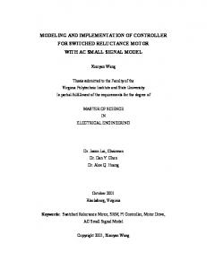
Figure 3: The output of system, 𝑠 = 𝑛 = 3.
(35)
= 𝐷 + 𝐶(𝑧𝐼 − 𝐴 𝐹 ) 𝐵𝐹 . ̂ satisfying (35) can be used in Figure 2. Convenient Thus, 𝐷(𝑧) for using in engineering, we can also design the state equation ̂ of 𝐷(𝑧). 4.2. Parameter Matrix 𝑅(𝑧) Design. To accomplish the controller design, the rest of the work is to design the parameter matrix 𝑅(𝑧) based on the requirements of the system performance. Suppose that the system error is defined as 𝑒 = 𝑤 − 𝑦 and the requirement of performance is to decrease 𝑒. Recall the system structure shown in Figure 2 and notice that the dynamics of the system is subject to the following equation: ̂ (𝑧) 𝑦 (𝑧) = 𝑆 (𝑧) ℎ (𝑧) + 𝐻 (𝑧) 𝜙 (𝑧) 𝐷
(36)
̂ ̂ ̂ in which 𝑆(𝑧) = 𝑉(𝑧)𝑅(𝑧) 𝐷(𝑧), 𝐻(𝑧) = 𝐼 − 𝑉(𝑧)𝑅(𝑧), and −1 𝜙(𝑧) = [𝐼 𝐶(𝑧𝐼 − 𝐴) 𝑑(𝑧)]. Hence, it has become a norm optimization problem to design the parameter matrix 𝑅(𝑧) [30]. We can choose a matrix 𝑅(𝑧) satisfying that the H∝ ̂ norm of the matrix 𝐼− 𝑉(𝑧)𝑅(𝑧) is minimum. In general, 𝑅(𝑧) need meet the conditions of stability and be simple enough to satisfy the practical requirements. All in all, we can choose 𝑅(𝑧) as a constant matrix −1
−
𝑅 = (𝐷𝑥 + 𝐶𝑥 (𝐼 − 𝐴 𝑥 ) 𝐵𝑥 ) 𝐺
(37)
with (∙)− representing the pseudoinverse. When 𝐷𝑥 + 𝐶𝑥 (𝐼− − 𝐴 𝑥 )−1 𝐵𝑥 is nonsingular, 𝑅 = (𝐷𝑥 + 𝐶𝑥 (𝐼 − 𝐴 𝑥 )−1 𝐵𝑥 ) 𝐺 is −1 equal to 𝑅 = (𝐷𝑥 + 𝐶𝑥 (𝐼 − 𝐴 𝑥 )−1 𝐵𝑥 ) 𝐺.
5. An Academic Example In this section, we apply the achieved results to an academic example. Our major purpose is to demonstrate the applicability and effectiveness of the residual generator-based
controller. We assume the system matrixes in the state space to be as follows: 0 0 −0.006 𝐴 = [1 0 −0.11 ] , [0 1 −0.6 ] 𝐶 = [1.6 1.5 0.5] , 𝑑 (𝑘) ∼ 𝑁 (0, 0.012 ) ,
1 0 𝐵 = [0.18 0.33] , [0.47 0.8 ] 𝐷 = zeros (1, 2) ,
(38)
𝑛 (𝑘) ∼ 𝑁 (0, 0.012 ) .
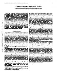
𝑁(𝜇, 𝜎2 ) presents normal distribution whose mean is 𝜇 and variance is 𝜎2 . Note that we just use the system model to generate the indispensable inputs and outputs as the available test data, and we do not use the system matrixes 𝐴, 𝐵, 𝐶, and 𝐷 and the noises to design the controller. The simulation procedure of the data-driven based controller is as follows. At first, simulate the academic example, and collect 1000 samples of the test data with the reference excitation. Then, identify the parity space using Algorithm 1. Based on the relationship between the parity space and DO, we construct an observer-based residual generator, advanced to design the controller. To demonstrate the application of the controller, we choose the simulation time as 𝑇 = 1000 s and sample time as 𝑇𝑠 = 1 s. And introduce disturbances 𝑑(𝑘) = 0.1 and 𝑛(𝑘) = 0.1, when 𝑡 = 500 s and 𝑡 = 600 s, respectively. Figure 3 shows the output signal collected from experiment with 𝑠 = 𝑛. And, as can be seen from Figure 3, the performance of the controller system is very well, the response speed of unit step is very fast, and disturbances have been suppressed effectively. More generally, we choose that 𝑠 > 𝑛, 𝑠 = 5, for instance, and the output signal is shown in Figure 4. We can learn from Figure 4 that the disturbances have been suppressed effectively; however, when the reference excitation is unit step signal, the overshoot is a bit larger. Thus, we reduce the order
Mathematical Problems in Engineering
7 directly identified from available process measurements without generating system model. We constructed the residual generator based on the relationship between DO and the parity vector, obtained directly from process measurements using the advanced SIM. Finally, the applications and effectiveness are demonstrated by applying the scheme and algorithms to an academic example. Besides, our future work is studying a scheme dealing with a real-time system [31, 32].
Output versus reference 1.2
Amplitude
1 0.8 1 0.6
0.8 0.6
0.4
Conflict of Interests
0.4 0.2 0
0.2 0
95
−0.2
The authors declare that there is no conflict of interests regarding the publication of this paper.
100 105 110 115
Acknowledgments 0
200
400
600
800
1000
Sample Reference Output
References
Figure 4: The output without order reduced, 𝑠 = 5. Output versus reference 1.2
1
Amplitude
0.8
1 0.8
0.6
0.6 0.4
0.4 0.2
0.2
0
0 −0.2
95 0
200
100 105 110 115 400
600
800
The authors acknowledge the support of China Postdoctoral Science Foundation Grant no. 2012M520738 and Heilongjiang Postdoctoral Fund no. LBH-Z12092.
1000
Sample Reference Output
Figure 5: The output with order reduced, 𝑠 = 5.
of the residual generator based on Algorithm 2, and then we generate the outputs of the system as Figure 5 shows. It is easy to learn that the overshoot become a smaller one.
6. Conclusion In this paper, we deal with the controller design for LTI system based on data-driven techniques. The scheme proposed is summarized in the form of several algorithms to be convenient for the readers learning the scheme proposed. The core of this paper is embedding residual generation aiming for FDI in the feedback control loop and structuring the observerbased residual generator based on data-driven approaches
[1] X. Xie, S. Yin, H. Gao, and O. Kaynak, “Asymptotic stability and stabilisation of uncertain delta operator systems with timevarying delays,” IET Control Theory & Applications, vol. 7, no. 8, pp. 1071–1078, 2013. [2] X. Zhao, L. Zhang, P. Shi, and M. Liu, “Stability and stabilization of switched linear systems with mode-dependent average dwell time,” IEEE Transactions on Automatic Control, vol. 57, no. 7, pp. 1809–1815, 2012. [3] Q. Zhou, S. Peng, X. Shengyuan, and L. Hongyi, “Observerbased adaptive neural network control for nonlinear stochastic systems with time-delay,” IEEE Transactions on Neural Networks and Learning Systems, vol. 24, pp. 71–80, 2013. [4] X. Zhao, L. Zhang, P. Shi, and H. Reza Karimi, “Novel stability criteria for T-S fuzzy systems,” IEEE Transactions on Fuzzy Systems, vol. 21, no. 6, pp. 1–11, 2013. [5] H. Li, J. Yu, C. Hilton, and H. Liu, “Adaptive sliding mode control for nonlinear active suspension vehicle systems using TS fuzzy Approach,” IEEE Transactions on Industrial Electronics, vol. 60, pp. 3328–3338, 2013. [6] Q. Zhou, P. Shi, J. Lu, and S. Xu, “Adaptive output-feedback fuzzy tracking control for a class of nonlinear systems,” IEEE Transactions on Fuzzy Systems, vol. 19, no. 5, pp. 972–982, 2011. [7] S. Yin, S. Ding, A. Haghani, H. Hao, and P. Zhang, “A comparison study of basic datadriven fault diagnosis and process monitoring methods on the benchmark Tennessee Eastman process,” Journal of Process Control, vol. 22, pp. 1567–1581, 2012. [8] S.-L. J¨ams¨a-Jounela, “Future trends in process automation,” Annual Reviews in Control, vol. 31, no. 2, pp. 211–220, 2007. [9] X. Zhao, P. Shi, and L. Zhang, “Asynchronously switched control of a class of slowly switched linear systems,” Systems & Control Letters, vol. 61, no. 12, pp. 1151–1156, 2012. ˚ om, T. H¨agglund, and C. C. Hang, “Automatic tun[10] K. J. Astr¨ ing and adaptation for PID controllers—a survey,” Control Engineering Practice, vol. 1, no. 4, pp. 699–714, 1993. [11] T. Yamamoto, K. Takao, and T. Yamada, “Design of a datadriven PID controller,” IEEE Transactions on Control Systems Technology, vol. 17, no. 1, pp. 29–39, 2009. [12] S. Yin, Data-Driven Design of Fault Diagnosis Systems, VDIVerlag, D¨usseldorf, Germany, 2012.
8 [13] V. H. Nguyen and J.-C. Golinval, “Fault detection based on Kernel Principal Component Analysis,” Engineering Structures, vol. 32, no. 11, pp. 3683–3691, 2010. [14] G. Lee, C. Han, and E. S. Yoon, “Multiple-fault diagnosis of the Tennessee Eastman process based on system decomposition and dynamic PLS,” Industrial and Engineering Chemistry Research, vol. 43, no. 25, pp. 8037–8048, 2004. [15] R. Muradore and P. Fiorini, “A PLS-based statistical approach for fault detection and isolation of robotic manipulators,” IEEE Transactions on Industrial Electronics, vol. 59, no. 8, pp. 3167– 3175, 2012. [16] S. X. Ding, Mode-Based Fault Diagnosis Techniques, Springer, Berlin, Germany, 2008. [17] S. X. Ding, P. Zhang, A. Naik, E. L. Ding, and B. Huang, “Subspace method aided data-driven design of fault detection and isolation systems,” Journal of Process Control, vol. 19, no. 9, pp. 1496–1510, 2009. [18] A. S. Naik, S. Yin, S. X. Ding, and P. Zhang, “Recursive identification algorithms to design fault detection systems,” Journal of Process Control, vol. 20, no. 8, pp. 957–965, 2010. [19] S. X. Ding, N. Weinhold, P. Zhang, E. L. Ding, T. Jeinsch, and M. Schultalbers, “Integration of FDI functional units into embedded tracking control loops and its application to FDI in engine control systems,” in Proceedings of the IEEE International Conference on Control Applications (CCA ’05), pp. 1299–1304, Toronto, Canada, August 2005. [20] N. Weinhold, S. X. Ding, T. Jeinsch, and M. Schulalbers, “Embedded model-based fault diagnosis for on-board diagnosis of engine management systems,” in Proceedings of the IEEE Conference on Decision and Control, pp. 1206–1211, Toronto, Canada, 2005. [21] S. X. Ding, G. Yang, P. Zhang et al., “Feedback control structures, embedded residual signals, and feedback control schemes with an integrated residual access,” IEEE Transactions on Control Systems Technology, vol. 18, no. 2, pp. 352–366, 2010. [22] K. Zhou and J. C. Doyle, Essentials of Robust Control, PrenticeHall, Upper Saddle River, NJ, USA, 1998. [23] H. Li, X. Jing, and H. R. Karimi, “Output-feedback based H-infinity control for active suspension systems with control delay,” IEEE Transactions on Industrial Electronics, vol. 61, pp. 436–446, 2014. [24] E. Y. Chow and A. S. Willsky, “Analytical redundancy and the design of robust failure detection systems,” IEEE Transactions on Automatic Control, vol. 29, no. 7, pp. 603–614, 1984. [25] P. Zhang and S. X. Ding, “Disturbance decoupling in fault detection of linear periodic systems,” Automatica, vol. 43, no. 8, pp. 1410–1417, 2007. [26] S. Yin, G. Wang, and H. Karimi, “Data-driven design of robust fault detection system for wind turbines,” Mechatronics, 2013. [27] J. Wang and S. J. Qin, “A new subspace identification approach based on principal component analysis,” Journal of Process Control, vol. 12, no. 8, pp. 841–855, 2002. [28] S. X. Ding, S. Yin, and Y. Wang, “Data-driven design of observers and its applications,” in Proceedings of the 18th IFAC World Congress, Milano, Italy, 2011. [29] J. Wang and S. J. Qin, “Closed-loop subspace identification using the parity space,” Automatica, vol. 42, no. 2, pp. 315–320, 2006. [30] S. Yin, H. Luo, and S. Ding, “Real-time implementation of faulttolerant control systems with performance optimization,” IEEE Transactions on Industrial Electronics, vol. 64, pp. 2402–2411, 2014.
Mathematical Problems in Engineering [31] S. Yin, S. X. Ding, A. H. A. Sari, and H. Hao, “Data-driven monitoring for stochastic systems and its application on batch process,” International Journal of Systems Science, vol. 44, no. 7, pp. 1366–1376, 2013. [32] S. Yin, X. Yang, and H. R. Karimi, “Data-driven adaptive observer for fault diagnosis,” Mathematical Problems in Engineering, vol. 2012, Article ID 832836, 21 pages, 2012.
Advances in
Operations Research Hindawi Publishing Corporation http://www.hindawi.com
Volume 2014
Advances in
Decision Sciences Hindawi Publishing Corporation http://www.hindawi.com
Volume 2014
Journal of
Applied Mathematics
Algebra
Hindawi Publishing Corporation http://www.hindawi.com
Hindawi Publishing Corporation http://www.hindawi.com
Volume 2014
Journal of
Probability and Statistics Volume 2014
The Scientific World Journal Hindawi Publishing Corporation http://www.hindawi.com
Hindawi Publishing Corporation http://www.hindawi.com
Volume 2014
International Journal of
Differential Equations Hindawi Publishing Corporation http://www.hindawi.com
Volume 2014
Volume 2014
Submit your manuscripts at http://www.hindawi.com International Journal of
Advances in
Combinatorics Hindawi Publishing Corporation http://www.hindawi.com
Mathematical Physics Hindawi Publishing Corporation http://www.hindawi.com
Volume 2014
Journal of
Complex Analysis Hindawi Publishing Corporation http://www.hindawi.com
Volume 2014
International Journal of Mathematics and Mathematical Sciences
Mathematical Problems in Engineering
Journal of
Mathematics Hindawi Publishing Corporation http://www.hindawi.com
Volume 2014
Hindawi Publishing Corporation http://www.hindawi.com
Volume 2014
Volume 2014
Hindawi Publishing Corporation http://www.hindawi.com
Volume 2014
Discrete Mathematics
Journal of
Volume 2014
Hindawi Publishing Corporation http://www.hindawi.com
Discrete Dynamics in Nature and Society
Journal of
Function Spaces Hindawi Publishing Corporation http://www.hindawi.com
Abstract and Applied Analysis
Volume 2014
Hindawi Publishing Corporation http://www.hindawi.com
Volume 2014
Hindawi Publishing Corporation http://www.hindawi.com
Volume 2014
International Journal of
Journal of
Stochastic Analysis
Optimization
Hindawi Publishing Corporation http://www.hindawi.com
Hindawi Publishing Corporation http://www.hindawi.com
Volume 2014
Volume 2014