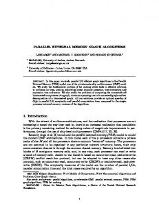
Reducing Memory Requirements of Stream Programs by Graph ...
Recommend Documents
Nov 9, 2013 - a whole crowd. We will show that this results in low memory re- quirements and allows for painless rig and animation transfer. 2 Related work.
*Louisiana State University, Baton Rouge, LA 70803, USA. ([email protected]) ...... International Conference on Supercomputing, St. Malo, France, pp. 238-253.
Abstract. Scalable Montgomery modular multiplier is able to per- form multiprecision Montgomery modular multiplications in limited hardware, but it requires ...
this in a deterministic list ranking algorithm. Department of Computer Science, Box 1910, Brown Univer- sity, Providence, RI 02912{1910. ySupported in part by ...
dynamically adjusting the memory bit-width to the number of bits changed per pixel. ... phone, has elevated needs for low-energy video encoding hardware.
programs. In this paper, we demonstrate with four case studies how ... The use of graphs to model dynamic structures is ubiquitous in computer science: ...
[6] Thomas H. Cormen, Charles E. Leiserson, Robert L. Rivest & Clifford Stein (2009): Introduction to Algo- rithms, third edition. The MIT Press. [7] R. J. Duffin ...
S. Pan and C. Zhang are with the Centre for Quantum Computation and Intelligent Systems, FEIT, University ... Sydney, NSW 2007, Australia (e-mail: [email protected]; ..... a set of frequent subgraphs to transfer graph stream into vec- tor
My parents, Hong Joon Ahn and Keum Sook Seo, devoted themselves to my education and have been my ..... personalized services, as well as a wide range of applications. ... makes computation cheap and bandwidth expensive. Moore's law ...
Telelogic Doors, IrQA, or IBM Requisite Pro mainly ... In Section 3, we describe our graph-based vi- ... one screen, the exploration is executed in top-down.
Impact changes analysis; Graph theory PageRank algorithm. I. INTRODUCTION. Defining requirements for large complex systems and managing existing ...
E-mail address: {goodrich,nodari}@ics.uci.edu. Abstract. In this paper, we study parallel I/O efficient graph algorithms in the Parallel. External Memory (PEM) ...
An industry standard, Advanced Configuration and Power Interface (ACPI) defining an open interface used by the OS to control power/energy consumption is ...
Sep 25, 2014 - revoked, or that the person has diplomatic immunity. A possible ... Suppose that we add atoms (p : pardon) and (d : diplomat) to program P4.
Sep 25, 2014 - positive programs, we show that the causal justifications obtained for a ...... of this example is incorporating some mechanic device to stop the.
An electronic-requesting system was implemented in April 2013. ... In December 2013, 55 (76%) were electronically requested and 17 (24%) .... Sign up in the.
FIGURE 12.1: Complete view of the graph stream visualization interface featuring tweets from President Obama's speech on the U.S. economy on. 07/24/2013 ...
The Leeds Teaching Hospital NHS Trust policy on mid-stream urine ... under a licence) please go to http://group.bmj.com/group/rights-licensing/permissions.
REDUCING RISK. Reducing the risk of emergence of pandemic influenza me
ation a. 7 d. 8 t n. STREAM 1. Background document ...
Overgeneral autobiographical memory (Williams, 1996) refers to a phenomenon ... Correspondence should be addressed to Philip J. Barnard, MRC Cognition ...
Apr 14, 2011 - Testimonial accuracy. To assess the quality of witness reports in different interview conditions, we calculated testimonial accuracy by dividing ...
Show off your creative genius and marketing strategy skills as the STREAM. Marketing ... Create and submit progress repo
Oct 16, 2009 - An algorithm that maps unstructured stream programs. onto heterogeneous .... ing algorithm a set of basic connected sets [25], each of which. specifies ..... reservoir.com/r-stream.php) is a proprietary high level com-. piler for ...
Sep 30, 2010 - sed on max-flow/min-cut for solving a wide range of pro- ... development with the arrival of a fast max-flow algorithm [6]. At the same time, the ...
Reducing Memory Requirements of Stream Programs by Graph ...
stream graph, and the underlying data-flow formalism en- ables powerful ..... The exploration algorithms are written in Python and exe- cuted using Python 2.5.4 ...
Reducing Memory Requirements of Stream Programs by Graph Transformations Pablo de Oliveira Castro, St´ephane Louise CEA, LIST, Embedded Real Time Systems Laboratory, F-91191 Gif-sur-Yvette, France; [email protected][email protected] ABSTRACT Stream languages explicitly describe fork-join parallelism and pipelines, offering a powerful programming model for many-core Multi-Processor Systems on Chip (MPSoC). In an embedded resource-constrained system, adapting stream programs to fit memory requirements is particularly important. In this paper we present a new approach to reduce the memory footprint required to run stream programs on MPSoC. Through an exploration of equivalent program variants, the method selects parallel code minimizing memory consumption. For large program instances, a heuristic accelerating the exploration phase is proposed and evaluated. We demonstrate the interest of our method on a panel of ten significant benchmarks. Using a multi-core modulo scheduling technique, our approach lowers considerably the minimal amount of memory required to run seven of these benchmarks while preserving throughput.
KEYWORDS: Stream Languages, Data Flow, Memory, Graph Transformations.
1. INTRODUCTION The recent low-consumption Multi-Processors Systems on Chip (MPSoC) enable new computation-intensive embedded applications. Yet the development of these applications is impeded by the difficulty of efficiently programming parallel applications. To alleviate this difficulty, two issues have to be tackled: how to express concurrency and parallelism adapted to the architecture and how to adapt parallelism to constraints such as buffer sizes and throughput requirements. Stream programming languages [10][15][11] are particularly adapted to describe parallel programs. Fork-join parallelism and pipelines are explicitly described by the
Denis Barthou University of Bordeaux - Labri / INRIA 351, cours de la Lib´eration, Talence, F-33405 France; [email protected] stream graph, and the underlying data-flow formalism enables powerful optimization strategies. As an example, the StreamIt [10] framework defines transformations of dataflow programs guided by greedy heuristics and enhancing parallelism through fission/fusion operations. However, to our knowledge, there is no method that explores the design space based on the different expressions of parallelism and communication patterns. The main difficulty comes from the definition of a space of semantically equivalent parallel programs and from the computational complexity of such exploration. In this paper we propose a design space exploration technique that generates, from an initial program, a set of semantically equivalent parallel programs, but with different buffer, communication and throughput costs. Using an appropriate metric, we are able to select among all the variants, the one that best fits our requirements. We believe that our approach is applicable to memory, communication and throughput requirements, yet this paper focuses only on memory requirements. The buffer requirements of stream programs depend not only on the rates of actors but also on the chosen mapping and scheduling. We illustrate the memory reduction achieved by our technique using the modulo scheduling execution model. Memory reduction on modulo scheduling has already been studied by Choi et al[6]. They propose an integer linear programming (ILP) approach to tackle the Memory-constrained Processor Assignment for minimizing Initialization Interval (MPA-ii) problem and measure the minimal memory requirements that their solution require. By exploring the memory design space of the input programs before mapping them with Choi et al. approach, we further reduce the memory requirements (sometimes as much as 80%). Section 2 introduces the stream formalism used. The transformations producing semantically equivalent pro-
gram variants are described in Section 3. Section 4 presents the exploration algorithm built upon these transformations and the algorithm termination proof. Section 5 reviews the MPA-ii problem that we use to illustrate the benefits of our exploration method and the metric used during our exploration. In Section 6 we describe our experimental methodology and results. Finally, Section 7 presents related works.
2. FORMALISM Our formalism, very close to StreamIt[10], describes a program using a cyclo-static data flow (CSDF) graph[4] where nodes are actors that are fired periodically and edges represent communication channels. Consider the example of stream graph in fig. 1. Different types of actors are considered. Source I and Sink O actor nodes model respectively a programs input and output. The source produces a stream of inputs elements, whereas the sink consumes all the elements it receives. If a source produces always the same element it is a constant source C. A sink whose elements are never observed is called a trash sink T. Functions in the imperative programming paradigm are replaced by Filter actors F(c1 , p1 ). Each filter has one input and one output, and an associated pure (without internal state) function f . Each time there are at least c1 elements on the input, the filter is fired: the function f consumes the c1 input elements and produces p1 elements on the output. Then there are nodes that dispatch and combine streams of data from multiple filters, routing data streams through the program and reorganizing the order of elements within a stream. Join round-robin J(c1 . . . cn ) gathers the elements received on its n inputs and writes them on its output. In its k th firing the node consumes cu ∈ N? elements on its uth input, with u = (k mod n) + 1 and writes them on its output. When the node has consumed elements on all its inputs, it has completed a cycle. Split round-robin S(p1 . . . pm ) dispatches the elements it receives on its input among its m outputs. In its k th firing the node takes pv ∈ N? elements on its input, with v = (k mod m) + 1 and writes them to the v th output. Duplicate D(m) has one input and m outputs. Each time this node is fired, it takes one element on the input and writes it to every output, duplicating its input m times.
2.1. Schedulability We can schedule a CSDF graph in bounded memory if it has no deadlocks (it is live) and if it admits a steady-state schedule (it is consistent) [4][14]. A graph deadlocks if the number of elements received by any sink remains bounded
p1
I
c01
p01
F
J
S p2
c1
c02
G
p02
c03
H
p03
c2
Figure 1. A Simple Stream Graph: the split node S consumes alternatively p1 and p2 elements from I. These are passed to filters F and G (that may be scheduled concurrently) and their outputs are combined by the join node J and passed to H.
no matter the number of elements streamed through the sources. A graph is consistent if it admits a steady-state schedule, that is to say a schedule during which the amount of buffered elements between any two nodes remains bounded. A consistent CSDF graph G with NG nodes admits a positive repetition vector q~G = [q1 , q2 , . . . , qNG ] where qi represents the number of cycles executed by node i in its steady-state schedule. Given two nodes u, v connected by edge e. We note β(e) the elements exchanged on edge e during a steady-state schedule execution. If node u produces prod(e) elements per cycle on edge e and node v consumes cons(e) elements per cycle on edge e, β(e) = prod(e) × qu = cons(e) × qv
(1)
2.2. Executing a CSDF on a Multi-Core System There are different approaches to map and execute a CSDF graph [10][14]. In this paper we use the Stream Graph Modulo Scheduling (SGMS) approach for multi-core systems proposed in [13]. SGMS is similar to classical modulo scheduling for instructions, each node u is assigned a single processing element (PE) and is scheduled on a particular activation stage stageu . Stages are activated gradually, forming a software pipeline that executes the different nodes in the stream concurrently. The first phase of SGMS is the PE assignment. By solving an ILP problem, we assign to each PE a group of nodes, so that every node is assigned to a exactly one PE and the computing load of the nodes is balanced among the PEs. The second phase of SGMS is the stage assignment. Its role is to select an efficient temporal schedule for the software pipeline. This is achieved by enforcing two simple rules: • Preservation of data dependences: The stage number of a producing actor must be greater or equal than the stage number of the consuming actor. • Overlapping transfer latencies and computation time: Two actors u, v that are mapped to different PEs and
stage 1
P1 DMA
I
1
S
1
stage 2
F
1
I
2
S
1 S − → G
P2
2
stage 3
F
2
1 F − → J
I
3
S
2 S − → G
3
F
3
2 F − → J
G1 J 1 H 1
... ...
Definition 2 A transformation T preserves the semantics of G if T preserves consistency, liveness and if for the same inputs, the graph generated by T , G0 , produces at least the same outputs as G.
...
Figure 2. SGMS Software Pipeline on 2 PEs with a DMA for the Graph in fig. 1: the indexes indicate the current node appearance. An appearance of node N correspond to qN cycles, that is to say an execution in the steady-state schedule. connected by e need a DMA operation or a network operation to transfer the data from one PE to the other. In this case we schedule the data transfer of e in stagee and we enforce that stageu < stagee < stagev . By scheduling the data transfer on a different stage than the consumer and producer on the software pipeline, we ensure that data transfer latencies and computation time are efficiently overlapped. In fig. 2, we show one possible SGMS schedule for the program in fig. 1. Nodes I, S, F are assigned to processing element P 1 and nodes G, J, H are assigned to processing element P 2.
3. SEARCH SPACE In this section we present the transformations that are used to generate variants preserving the semantics of the input program.
3.1. Graph Transformation Framework The graph transformation framework presented here follows the formulation given in [3]. A transformation T applied on a graph G, generating a graph G0 is denoted T G − → G0 . It is defined by a matching subgraph L ⊆ G, a replacement graph R ⊆ G0 and a glue relation g that binds the frontier edges of L (edges between nodes in L and nodes in G\L) to the frontier edges of R. The graph transformation works by deleting the match subgraph L from G thus obtaining G\L. After this deletion, all the edges between G\L and L are left dangling. We then use the glue relation to paste R into G\L obtaining G0 . We will describe transformations by giving the match and replacement subgraphs as in fig. 3. The input and output edges will be denoted ix and oy in both graphs. The natural correspondence between the ix (resp. oy ) of L and R gives the glue relation. Definition 1 A derivation of a graph G0 is a chain of transformations that can be successively applied to G0 : T0 Tn G0 −→ G1 . . . −−→ . . ..
The first two properties ensure that the transformation preserves the schedulability of the graph (cf. sec. 2). The last property ensures that the transformation does not change the observable outputs of the program. Because some of our transformations “relax” the consumption or production rates of split and join nodes, a variant may produce more values on the outputs than the original graph. If this was not allowed we would lose many desirable transformations. Besides, they still preserve the semantics since the extra values can be safely ignored by redirecting them to a fictitious Trash node (the number of extra values is known at compile time). A formal definition of the semantic preservation of CSDF transformations is found in [7], also an illustration of the interest of allowing extra values is provided.
3.2. Simplifying Transformations These transformations, remove nodes with either no effect or non-observed computations, and separate split-join structures into independent ones. Dead code elimination(fig. 3(f)) is a dead-code elimination for stream graphs. A node for which all outputs go to a Trash can be replaced by a Trash itself without affecting the semantics. This transformation progressively removes nodes whose outputs are never observed. Constant propagation(fig. 3(i)) when a constant source is split we can eliminate the split duplicating the constant source. RemoveJS / RemoveSJ / RemoveD (not shown in the figure) are very simple transformations which remove nodes whose composed effect is the identity : a split and a join of identical consumption and productions, a single branch dup, a single branch split, etc. CompactSS/CompactDD/CompactJJ (fig. 3(e)) fuse together a hierarchy of Splits, Joins or Duplicate nodes. CompactDD is always possible, we can replace any tree of Duplicate nodes by a single Duplicate node which copies its input stream to every output edge of the original tree. CompactSS is possible when when the lower split productions sum is equal to the production on the edge connecting the lower and upper splits. CompactJJ is possible when when the upper join consumptions sum is equal to the consumption on the edge connecting the lower and upper joins.
i1 i1
i1
⇒
F
S
c1
c1
...
c1c1 p1p1
F
p1
p1
J
o1
c1
...
in
p1
o1
o1
S
. . . om
N
p1 + · · · + pm
⇒ N
D
on1. . o. nm
o11. . .on1
. . . om
c1
J
...m...
D
p1
S
pm
o1 . . . okok+1. . .om
p
S
c1
p1
S
p
i1
S
J
J
cn
c1
S
S
p1
pm
o1 . . . okok+1. . .om
o1
S
N p1
in
T
⇒
T
T
(f) Dead-code elim.
in
c2
S p1
⇒
pm
i2 . . .
i1
cn
c1 − p1
J
cn
C ... C
C ⇒
pm
p2
o2 . . . om
(g) Synchronization removal
in0 . . . inn
S
pm
J
p
in0 . . . inn
⇒
i2 . . .
i1
S
p
. . . o2.k=m o1 . . o. 2k−1 o2 . . . o2k
(e) CompactSS
⇒ p1
p
o1 . . . om om+1. . . o2m o1 . . . om om+1. . . o2m
o1m. . o. nm
i1 . . . ij ij+1 . . . in
cn
o1
S
(c) ReorderS
(d) InvertDN
i1 . . . ij ij+1 . . . in
p
i1
i1
D
o11. . o. 1m
J
o1
p
⇒
cm1 cmn
J
pm
S
p
...
(b) InvertJS
i1
...n...
pn1 pnm
... c11 c1n
p1
i1
S
p11 p1m
⇒
(a) SplitF
N
S
c1
F
in i1
cn
J
...
i1
o1
(h) BreakJS
S
pm
o2 . . . om
S out1 . . .outn
out1 . . .outn
(i) Constant prop.
Figure 3. Set of Transformations Considered: each transformation is defined by a graph rewriting rule. Node N is a wildcard for any arity compatible node.
Synchronization Removal(fig. 3(g)) is possible when the sum of the join Pconsumptions P is equal to the sum of the split productions: x cx = y py . The idea behind this transformation is to find a partition of the join consumptions and aPpartition of P the split production so that their sum is equal: x≤j cx = y≤k pk . In that case we can split the JoinSplit in two smaller and independant Join-Split. P P BreakJS(fig. 3(h)) is triggered when x cx = y py but no partition of the productions/consumptions can be found. In that case the transformation breaks the split or join edge with the largest consumptions. BreakJS breaks Join-Split junctions into smaller constituents, often triggering Synchronization Removal separating the Join-Split junction into two smaller junctions.
concurrency introduced by SplitF is parametric. Multiple splitting of the same filter are useless, since they can be achieved with a single SplitF of greater arity.
3.3. Restructuring Transformations
The transformation is admissible P in two cases: 1- Each pj is a multiple of C = i ci , the transformation is admissible choosing pij = ci .pP j /C, cji = ci . 2- Each ci is a multiple of P = j pj , the transformation is admissible choosing pij = pj , cji = pj .ci /P .
These transformations restructure communication patterns, alone they do not reduce the memory requirements, but they can rewrite the graph and trigger some of the previous transformations. SplitF(fig. 3(a)) This transformation splits a filter on its input. SplitF introduces split-join parallelism in the programs. Because filters are pure: we can compute each input block on a different filter concurrently. The degree of
InvertJS(fig. 3(b)) This transformation inverts join and split nodes. To achieve this it creates as many split nodes as inputs and as many join nodes as outputs. It then connects together the new split and join stages as shown in the figure. Intuitively, this transformation works by “unrolling” the cycle in the original nodes (examining consecutive executions of the nodes) so that a common period between the join and split stage emerges. The transformation make explicit the communication pattern in this common period, by inverting the split and join stages.
ReorderS/ReorderJ(fig. 3(c)) create a hierarchy of split (resp. join) nodes. In the following we will only discuss ReorderS. The transformation is parametric in the split arity f . This arity must divide the number of outputs, m = k.f . In the figure, we have chosen f = 2. We forbid
the trivial cases (k = 1 or f = 1) where the transformation is the identity. As shown in fig. 3(c), the transformation works by rewriting the original split using two separate stages: odd and even elements are separated then odd (resp. even) elements are redirected to the correct outputs. ReorderS and ReorderJ sometimes uncover possible simplifying transformations by explicitly separating elements by their f congruency (eg. even and odd elements when f = 2), InvertDN(fig. 3(d)) This transformation inverts a duplicate node and its children, if they are identical. Since all nodes are pure, their outputs depend only on their inputs; thus applying a process k times to the same input is equivalent to applying the process once making k copies of the output. This transformation eliminates redundant computations in a program.
4. EXPLORATION ALGORITHM The exploration is an exhaustive search of all the derivations of the input graph using our transformations. We use a branching algorithm with backtracking, as described recursively in algorithm 1. The exploration is particularly memory efficient because it never copies the graph when branching; transformations are in-place applied and in-place reverted when backtracking. We prove that this algorithm terminates by showing for any initial graph, that once a large enough recursion depth is reached, no transformations will satisfy the for all condition in statement 6. This follows from the fact that the transformations considered cannot produce infinite derivations. We prove this result formally in [7], yet a general idea of the proof follows. We start by constructing a function on graphs τ : (Graphs) 7→ (M(N), ), where M is the set of all finite multisets of N and its natural well-founded order[8]. We then show that for any of the transformations in sec. 3, τ (G) τ (G0 ). Using the wellfoundness of we prove that all the derivations are finite. Algorithm 1 E XPLORE(G) 1: Simpl ← {Dead Code, CompactSS, CompactJJ, ...} 2: Restr ← {SplitF, InvertJS, ReorderS, ...} 3: while ∃N ∈ G ∃S ∈ Simpl : S applicable at N do 4: G ← SN (G) 5: end while 6: for all N ∈ G and T ∈ Restr : T applicable at N do 7: G ← TN (G) 8: E XPLORE(G) 9: G ← R ESTORE(G) 10: end for
4.1. Dominance Rules Generated graphs G are often obtained through application of transformations operating on distinct part of the graph. In that case, applications of these transformations commute, meaning that the order in which they are applied does not change the resulting graph. Therefore only one of the possible permutations of the application order is explored. To select only one of the possible permutations, an arbitrary ordering (@) is defined on the transformations. We say that T1 dominates T2 if T1 @ T2 . A new transformation is applied only if it dominates all the earlier transformations that commute with it. A sufficient condition for an early transformation T1 to commute with a later transformation T2 is that the nodes that are matched by L2 were already present before applying T1 . This condition can be easily checked if nodes are tagged with a creation date during exploration.
4.2. Partitioning Heuristic Exhaustive search may take too much time on large graph instances. The optimization presented in the previous section alleviates this complexity issue; however for large graphs like Bitonic (370 nodes) or DES (423 nodes) in section 6, the exploration still takes too much time. To bound exploration time, we have implemented an heuristic combining our exploration with a graph partitioning of the initial program. For this to work, the metrics we optimize must be composable: there must exist a function f that verifies for every partition G1 , G2 of G, metric(G) = f (metric(G1 ), metric(G2 )). We show that reducing the initial program size, reduces the exploration maximal size. Our heuristic, based on this result works by partitioning the initial program in partitions of at most P SIZE nodes. If the metric we try to optimize is composable, exploring each partition separately, selecting the variant which optimizes f for each partition, and assembling them back together leads to valid results. To partition the graphs we use the freely available Metis [12] graph partitioning tool. The downside of this heuristic is that we loose the transformations involving nodes of different partitions. Yet our benchmarks in section 6 show that the degradation of the final solution is acceptable (except for very small partitions).
5. MEMORY REQUIREMENTS IN SGMS
5.1. Metrics
To evaluate our design-space exploration method, we apply it to memory reduction on a SGMS (cf. sec. 2) execution model.
In this section we propose a metric that selects candidates which improve the memory required for the modulo scheduling. From equations (2)(3) we observe that to reduce b(i) we can either reduce the stage difference between producers and consumers, δ(u, v), or we can reduce the elements exchanged during a steady-state execution, β(e).
The authors of [6] have studied the problem of reducing memory requirements in stream modulo scheduling. They introduce the problem MPA-ii, Memory-constrained Processor Assignment for minimizing Initiation Interval, and propose an ILP based solution; then they measure the minimal memory requirements achieved by their assignment. In the following we will show that if our exploration method is used we can significantly decrease these requirements. To compute the buffer sizes required by two nodes u and v communicating through an edge e, the authors in [6] consider two kinds of situations: • u and v are on the same PE, the output buffer of u can be reused by v. • u and v are on different PE, buffers may not be shared, since a DMA operation d is needed to transfer the data. The stage in which d is scheduled is noted staged . The number of elements produced by u and consumed by v on edge e during a steady-state execution is called β(e) and given by eq. (1). Furthermore, since multiple executions of the streams may be on flight in the pipeline at the same time, buffers must be duplicated to preserve data coherency. The number of buffer copies needed is the number of stages between the two nodes, δ(u, v) = stagev − stageu + 1. The output buffer requirements for all the nodes but Duplicate are, X δ(u, v) ∗ β(e) (2) out buf s(i) = ∀e∈outputs(i)
For Duplicate nodes, since the output is the same on all the edges, buffers can be shared by recipients, so the formula becomes : max∀e∈outputs(i) δ(u, v) ∗ β(e). The input buffer requirements are, X δ(v, d) ∗ β(e) in buf s(i) =
The authors of [6] already optimize the δ(u, v) when possible. We attempt to reduce b(i) by reducing β(e). To reduce the influence of the β(e) in the buffer cost we search the candidate that minimizes, maxbuf (G) = max∀e∈G β(e). if we have a tie between multiple candidates, we chose the P one that minimizes, totbuf (G) = ∀e∈G β(e). We note that these metrics are composable, as required by the partitioning heuristic described in section 4. Indeed given a partition G1 , G2 of G, we have maxbuf (G) = max(maxbuf (G1 ), maxbuf (G2 )) and totbuf (G) = totbuf (G1 ) + totbuf (G2 ).
6. RESULTS We consider a representative set of programs from the StreamIt benchmarks [1]: Matrix Multiplication, Bitonic sort, FFT, DCT, FMradio, Channel Vocoder. We also consider three benchmarks of our own: Hough filter and fine grained Matrix Multiplication (which both contain cycles in the stream graph), and Sobel filter. We first compute for each benchmark the minimal memory requirements per core for which an MPA-ii mapping is possible. We will use this first measure, MPAii mem, as our baseline. We then use our exploration method on each benchmark, and select the best candidate according to the metrics described in section 5. We compute the MPA-ii minimal memory per core requirements for the best candidate: Exploration MPAii mem. Finally we compute the memory requirements reduction using the following formula: (MPAii mem − Exploration MPAii mem) MPAii mem As shown in [13] it should be possible to integrate filter splitting in Choi et al. approach. Thus to make the comparison fair, we have not taken into account any further memory reduction achieved by SplitF transformation.
(3)
∀e∈dma inputs(i)
Combining (2)(3) we obtain the total memory requirements for a node b(i) = out buf s(i) + in buf s(i).
6.1. Memory Reduction The exhaustive search is used for all the benchmarks except DES and Bitonic for which we used the partitioning
heuristic, the partition maximum size (PSIZE) was set to 60 which was empirically determined as a good compromise between speed and quality of the solution. A significant memory reduction is achieved in seven out of the ten benchmarks. This means that in these seven cases the application can be executed with significantly less memory than using the approach in [6]: either a larger application can be mapped to the same architecture or an architecture with smaller memory requirements can be designed for this application. In terms of throughput, our method does not degrade the performance since we obtain similar II (initialization interval) values than bare MPA-ii. The experimental results obtained are summarized in fig. 4. We can distinguish three categories among the benchmarks: No effect (DCT, FM, Channel), in this first group of benchmarks, we do not observe any improvement. Indeed these programs make little use of split, join and duplicate nodes. They are almost filter only programs. Because our transformations operate essentially on data reorganisation nodes, they have no effect on these examples. The very small improvement in Channel is due to a single SimplifyDD that compacts a serie of duplicate nodes. Loop splitting (MM Fine, Hough), these two benchmarks contain cycles. Using our set of transformations we are able to split the cycles, as we demonstrate in fig. 5 for the Hough benchmark. This is particularly interesting in the context of modulo scheduling where cycles must be fused [13]. In the Hough selected variant, the cycle is broken in three smaller cycles: Thus after fusion, it has more fine-grained filters, and achieves smaller memory requirements. Dependencies breaking and communication reorganisation (MM coarse, MM fine, FFT, Bitonic, Sobel, DES), the other benchmarks show varying memory reductions, resulting from a better expression of communication patterns. Either non needed dependencies between nodes have been exposed, allowing for a better balance among the cores, or groups of split, join and dup have been simplified in a pattern that is less memory consumming.
6.2. Variation when Changing the Number of PE In this section we study the memory reduction variance depending on the number of cores in the target architecture. We can identify two categories: Plateau, graphs in this category, Bitonic, FFT, DES, show little change over the number of PEs. We observe in table 1 that for these graphs, maxbuf remains at the same level but totbuf has decreased.
Table 1. Metrics Variations between the Original Graph and the Best Selected Candidate (in number of elements). Benchmark
maxbuf variation
totbuf variation
MM fine MM coarse Bitonic DES FFT DCT FM Channel Sobel Hough
-1500 -1520 0 0 0 0 -6 0 -3392 -28000
-630 -209 -480 -3514 -184 0 +6 -17 -3841 -29933
Table 2. Measured Exploration Costs. Benchmark
Number of nodes
Exhaustive search time
Search time after partitioning (PSIZE = 60)
MM fine MM coarse Bitonic DES FFT DCT FM Channel Sobel Hough