These codes were discovered by D.E Muller and were provided with a decoding algorithm by Irving S. Reed in 1954. As telecommunication expanded, Reed-.
Journal of Computer Science 4 (10): 792-798, 2008 ISSN 1549-3636 © 2008 Science Publications
Reed-Muller Codec Simulation Performance Othman O. Khalifa, Aisha-Huassan Abdullah, N. Suriyana, Saidah Zawanah and Shihab A. Hameed Faculty of Engineering, International Islamic University Malaysia, P.O. Box 10, Jalan Gombak, 50728, Kula Lumpur, Malaysia Abstract: The approach to error correction coding taken by modern digital communication systems started in the late 1940’s with the ground breaking work of Shannon, Hamming and Golay. ReedMuller (RM) codes were an important step beyond the Hamming and Golay codes because they allowed more flexibility in the size of the code word and the number of correctable errors per code word. Whereas the Hamming and Golay codes were specific codes with particular values for q; n; k; and t, the RM codes were a class of binary codes with a wide range of allowable design parameters. Binary Reed-Muller codes are among the most prominent families of codes in coding theory. They have been extensively studied and employed for practical applications. In this research, the performance simulation of Reed-Muller Codec was presented. An introduction on Reed-Muller codes, were introduced that consists of defining the key terms and operation used with the binary numbers. Reed-Muller codes were defined and encoding matrices were discussed. The decoding process was given and some examples were demonstrated to clarify the method. The results and the performance of Reed-Muller encoding were presented and the messages been encoded using the defined matrices were shown. The simulation of the decoding part also been shown. The performance of Reed-Muller codes were then analyzed in terms of its code rate, code length and minimum Hamming distance. The analysis that performed also successfully examines the relationship between the parameters of ReedMuller coding. The decoding part of the Reed-Muller codes can detect one error and correct it as shown in the examples. Key words: Reed-Muller, code length, minimum Hamming distance, code rate INTRODUCTION
shown where Reed-Muller codes were introduced and the encoding and decoding matrices were constructed. The example of encoding and decoding a message using this code was shown. Apart from that, the encoding and decoding of Reed-Muller codes using MATLAB simulation was included under this part, in which the Reed-Muller codes were encoded in MATLAB and the output is compared with the theoretical one. The findings, discussion and analysis of the results were presented
Reed-Muller (RM) Codes are a family of linear error-correcting codes used in communications and are one of the oldest error correcting codes. However, error correcting codes play an important role in computational complexity theory and are very useful in sending information over long distances in which errors might occur in the message. These codes were discovered by D.E Muller and were provided with a decoding algorithm by Irving S. Reed in 1954. As telecommunication expanded, ReedMuller Codes become more prevalent as the needs for codes that can self-correct increased. Reed-Muller Codes has been widely used in many applications, as it is the most well known decomposable codes. In fact, Reed-Muller Code was used by Mariner 9 to transmit black and white photographs of Mars in 1972[1]. The outline of this paper is as follows. The coding theory of Reed-Muller codes and its parameters were presented. The implementation of these codes was
MATERIALS AND METHODS Coding theory of RM codes and its parameters: Reed-Muller can be defined as follow: r rank RM code R(r,m) is the code we get when the true table of a m elements Boolean function whose order is not larger than r is treated. In other words, an rth order of ReedMuller Code R(r, m) is the set of all binary string (vectors) of length n = 2m.
Corresponding Author: Othman O. Khalifa, Faculty of Engineering, International Islamic University Malaysia, Jalan Gombak, 50728 Kuala Lumpur, Malaysia
792
J. Computer Sci., 4 (10): 792-798, 2008 Case 1: If r is equal to 0, there are only one row in the encoding matrix, i.e., this row.
RM codes consist of three theorems that could be deduced from the definition above[2, 3].
Case 2: If r is equal to 1, a m rows (corresponding to the vectors x1, x2…, xm) are added to the R (0, m) encoding matrix.
Theorem 1: Assume that the check matrix of Hamming Code is H and its column vectors equal to the correspondent column serial number and then the dual code of increased Hamming code is: 1 Hg =
1
0
is a 1st order RM code R(1, m). Theorem 2: Generator matrix of (r+1) order RM codeR(r+1, m+1) order can be derived from the generator matrix (r+1) order of RM code R(r+1, m) and of rth order of RM code R(r, m) by equation below: G (r + 1, m ) 0
G (r + 1, m ) G (r, m )
Block length: n = 2m Information length: k =
(1)
x2 1 1 0 0 1 1 0 0 x3 1 0 1 0 1 0 1 0
The rows x1x2 = 11000000, x1x3 = 10100000 and x2x3 = 10001000 are added to form:
R(2,3) =
1
1 1 1 1 1 1 1 1
x1 x2 x3
1 1 1 1 0 0 0 0 1 1 0 0 1 1 0 0 1 0 1 0 1 0 1 0
x 1x 2 1 1 0 0 0 0 0 0 x1 x 3 1 0 1 0 0 0 0 0 x 2x3 1 0 0 0 1 0 0 0
(2)
i =0
rows is added to the R(r-1, m)
1 1 1 1 1 1 1 1 1 x1 1 1 1 1 0 0 0 0
R(1,3) =
Theorem 3: For any 0 r m-1, R(m-r-1, m) and R(r, m) are dual reciprocally. From these theorem stated above, it is known that RM codes are linear nonsystematic codes on GF(2) field. For every integer m and r 1,
1
Then, the row x1x2x3 = 10000000 is added to form: Cm
Minimum distance: d = 2m − r
(3)
1 x1 x2 x3 R(3,3) = x1x 2 x1x 3 x 2x3 x1x 2 x 3
(4)
As the definition stated before, an rth order of ReedMuller Code R(r,m) is the set of all binary string (vectors) of length n = 2m which associated with the Boolean polynomials p(x1, x2,…, xm) of degree at most r. The 0th-order of RM code, R(0, m) consists of the binary strings associates with the constant polynomial 0 and 1, R(0, m) = {0, 1} = Rep (2m). Thus, R(0, m) is just a repetition of either zeroes or ones at length 2m. On the other hand, the mth order of the RM code consists of all binary string of length 2m[3].
1 1 1 1 1 1 1 1
1 1 1 0 1 0 0 0
1 1 0 1 0 1 0 0
1 1 0 0 0 0 0 0
1 0 1 1 0 0 1 0
1 0 1 0 0 0 0 0
1 0 0 1 0 0 0 0
1 0 0 0 0 0 0 0
1
1 1 1 1 1 1 1 1 1 1 1 1 1 1 1 1
x1 x2 x3
1 1 1 1 1 1 1 0 0 0 0 0 0 0 0 0 1 1 1 1 0 0 0 1 1 1 1 0 0 0 0 0 1 1 0 0 1 0 0 1 1 0 0 1 1 1 0 0
x4 1 0 1 0 1 1 0 1 0 1 0 1 0 0 1 0 Hence, R(( 2, 4) = x1x2 1 1 1 1 0 0 0 0 0 0 0 0 0 0 0 0
Encoding and decoding matrices: Encoding matrix of R(r.m): Let the 1st row of the encoding matrix to be 1 and let the vector length 2m also equal to 1. There are several cases regarding this encoding matrix[4]:
x1x3 1 1 0 0 1 0 0 0 0 0 0 0 0 0 0 0 x1x4 1 0 1 0 1 1 0 0 0 0 0 0 0 0 0 0 x2x3 1 1 0 0 0 0 0 1 1 0 0 0 0 0 0 0 x2x4 1 0 1 0 0 0 0 1 0 1 0 0 0 0 0 0 x3x4 1 0 0 0 1 0 0 1 0 0 0 1 1 0 0 0
793
J. Computer Sci., 4 (10): 792-798, 2008 To encode a message using Reed-Muller code R (r, m), the dimension is given as: m
k =1+
1
+
m 2
+
+
m r
For decoding part, we must assume that the closest codeword in R(r, m) to the received message is the original encoded message[4]. Thus for errors (e) to be corrected in the received message, the distance between any two of the codeword in R(r, m) must be greater than 2e. The decoding process will check each row of the encoding matrix and uses majority logic to determine whether that row was used in forming the encoding message. Hence, it is possible to determine what is the error-less encoded message and the original message itself. This method of decoding is given by the following algorithm:
(5)
Consequently, the encoding matrix has k rows. For code R (r, m), let m = (m1, m2,…, mk) be a block, the encoded message Mc will be: Mc =
k i =1
(6)
miR i
Where: Ri = Encoding matrix of R (r, m)
Step 1: Choose a row in the R(r, m) encoding matrix. Find 2m-r characteristic vectors for that row and take the dot product of each rows with the encoded message.
For example, using R (1, 3) to encode m = (0110) will gives:
Step 2: Take the majority values of the dot products and assign that value to the coefficient of the row. (Repeat Step 1 and 2 for each row except the top row from the bottom matrix up).
0*(11111111)+1*(11110000)+1*(11001100)+0*(1010 1010) = 00111100 00000000 11110000 11001100
Step 3: Multiply each coefficient by its corresponding row and add the resulting vectors to form My. Add this result to the received encoded message. If the resulting vectors are more ones than zeros, then the top row's coefficient is 1, otherwise it is 0. To get the original encoded message, add the top row and multiply it by its coefficient My.
+00000000 00111100
Similarly, using R(2, 3) to encode m = (1010110) gives (0011100100000101). 1*(11111111)+0*(11110000)+1*(11001100)+0*(1010 1010)+1*(11000000)+1*(10000100) + 0*(100000000) = (01010011)
Step 4: Identify the errors. The vector formed by the sequence of coefficients starting from the top row of the encoding matrix and ending with the bottom row is the original message. To find the characteristic vectors of any row of the matrix, take the monomial r, which associated with the row of the encoding matrix. Then, take E to be the set of all xi that are not in the monomial r, but are in the encoding matrix. The characteristic vectors stated in Step 1 are the vectors corresponding to the monomials in xi and x i , such that exactly one of xi or x i is in each monomial for all xi in E. For example, the last row of the encoding matrix R(2, 4) is associated with x2x4, so the characteristic vectors correspond to the following combinations of x1, x2, x1 and x 2 : x1x 2 , x1x 2 , x1x 2 , x1x 2 . For example, given the original message is m = (0110). Using R (1, 3), then the encoded message is Mc = (00111100). Because the distance in R (1, 3) is 23-1 = 4, this code can correct one error. Let the encoded
11111111 00000000 11001100 00000000 11000000 10100000
+00000000 01010011
Decoding matrix of reed-muller code: Decoding Reed-Muller encoded messages is more complex compared to encoding process. The theory behind encoding and decoding is based on the distance between the vectors, i.e. the number of places in the two vectors that have different values. In R (r, m) code, the distance between any two codeword is 2m-r. 794
J. Computer Sci., 4 (10): 792-798, 2008 The sum of My and Me is (00111100)+(10111100) = (10000000):
message after the error be Me = (10111100). Hence, the characteristic vectors of the last row x3 = (10101010) are x1x 2 , x1 x 2 , x1 x 2 , x1 x 2 . The vector associated with x1 is (11110000), so x1 = (00001111). The vector associated with x2 is (11001100), so x 2 = (00110011):
equal
to
00111100 +10111100 10000000
x1= (11110000) → x = (00001111), x2 = (11001100) → x 2 = (00110011).
This message has more zeros than ones, so the coefficient of the 1st row of the encoding matrix is zero. Thus, putting all coefficients for the four rows of the matrix (0, 1, 1, 0) will get the original message of (0110). The error was in the 1st place of the error-free message Mc = (00111100).
Therefore, x1x2 = (11000000), x1 x 2 = (00110000), x x2 = (00001100) and x x 2 = (00000011). Taking the dot products of these vectors with Me will result in:
RESULTS The results of coding simulation were analyzed. By taking the example from the matrix R01, when m = 1, r = 0, the R01 code is the length-2 repetition code. We can see from the results that R01 yields R01 = [ 1 1]. It repeats the string 1 for length of 2. This is a simple verification. Let us see a more comprehensive example. R13 means that we have m = 3, thus we will have 2^3 codeword length of first order.
(11000000).(10111100) = 1, (00110000). (10111100) = 0 (00001100).(10111100) = 0, (00000011). (10111100) = 0
Thus, the coefficient of x3 is 0. Repeating the same process as above to the 2nd to last row of the matrix, x2 = (11001100), will get the characteristic vectors: x1x2 = (10100000) x1x 3 = (01010000) x1x 3 = (00001010 x1x 3 = (00000101)
This code has 4 rows since: k =
r i=0
m i
(7)
We can illustrate the calculation of rows here i is from 0-1 since r = 1. m = 3. So:
Taking the dot products of these vectors with Me, will result in:
k=
m i=0
(10100000).(10111100) = 0, (01010000).(10111100) = 1
m 3 3 3! = + = =1+ 3 = 4 i 0 1 0!(3 − 0!)
Thus, by comparing to the result, we can see that there are eight columns and four rows. As explained in the implementation section, we can then construct a
(00001010).(10111100) = 1, (00000101).(10111100) = 1
Hence, it can be concluded that the coefficient of x2 is 1. Repeating the same process as above for the second row of the matrix x1 = (11110000):
R23 code by simply adding
(10001000).(10111100) = 0, (00100010).(10111100) = 1 (01000100).(10111100) = 1, (00010001).(10111100) = 1
The coefficient for x1 is also 1. To get My, add 0* (10101010)+1* (11001100)+1* (11110000) = (00111100): 00000000 11001100 +11110000 00111100
795
m 3 3! = = = 3 r 2 2!(3 − 2!)
rows to R(r-1, m) = R(1, 3) encoding matrix. Thus, we will have 4+3 rows in the R23 code. These added rows consist of all possible reduced degree monomials that can be formed using the rows[5]. This applies to the rest of the R(r, m) codes that are constructed using the MATLAB simulation. If we compare the theoretical part of the encoding matrices with the simulated one, we can see the differences. One of them is the order of the rows is different and also the order at which the Boolean variables are applied also varies. This is according to[4] where it is stated that there is no specific order of preference to ordering the rows of the generator matrix of R(r,m). So, R(r,m) generator matrix is not unique.
J. Computer Sci., 4 (10): 792-798, 2008
Fig. 3: The graph of code length versus the code rate when the Rth order is equal 2
Fig. 1: The graph of code length versus the m positive integers
Fig. 4: The graph of code length versus the code rate when the Rth order is equal 3 This MATLAB simulation does not provide the mechanism to only produce output in the binary. Thus, we have to apply our basic knowledge on the modulo-2 addition operation. We can say that if the encoded message, encode1 in the MATLAB simulation is, encode1 = [0 1 1 2 0 1 1 2], the number 2 is considered as 0. This is because we apply 1 ⊕ 1 and yields 0. If the number is odd, let say 3, then the binary equivalent is 1 because 1⊕1⊕1 = 1. Let us proceed to the analysis of the relationship between the parameters of the codes. Figure 1 shows the relationship between the code length of the Reed-Muller codes and the m positive integer. As the m positive integer increases, we can see that the code length increases exponentially. This agrees with the given relation between code length and m that is code length = 2m. Figure 2 shows the relationship between the minimum Hamming distance and the order of the ReedMuller codes.
Fig. 2: The graph of minimum hamming distance, d versus the Rth order at different m values We will now briefly analyze the encoded message. If the input message is p bits, thus, we have to choose the R(r,m) codes at which the size of the input message, i.e., p bits is equal to the number of rows of the encoding matrix. For instance, for the input message that is given in the MATLAB simulation, we have input message of, m = [0 1 1 0], which has 4 bits. By using R13, the yielded result is the encoded message having the size of 8. But by using R22 which also has the same number of rows compared to the input size, the encoded message has the size of 4. This is due to the difference in the Boolean variables for each of the encoding matrix. In the encoded message result (in the attachment), the encoded message may produce output which i s no t i n b i nar y, b ut i n te ger n u mb er s. 796
J. Computer Sci., 4 (10): 792-798, 2008 recognized to be a new class of error correcting codes. RM codes were an important step beyond the Hamming and Golay codes because they allowed more flexibility in the size of the code word and the number of correctable errors per code word. Whereas the Hamming and Golay codes were specific codes with particular values for q; n; k; and t, the RM codes were a class of binary codes with a wide range of allowable design parameters. After the Mariner mission, RM codes fell out of favor within the coding community due to the discovery of more powerful codes. Recently there has been a resurging interest in RM codes because the high speed decoding algorithms are suitable for optical communications. To compare the theoretical part of the encoding matrices with the simulated one, we can see the differences. One of them is the order of the rows is different and also the order at which the Boolean variables are applied also varies. This is according to[4] where it is stated that there is no specific order of preference to ordering the rows of the generator matrix of R(r,m). So, R(r,m) generator matrix is not unique.
Fig. 5: Row versus column of the encoding matrices R(r, m) As shown, the minimum Hamming distance is plotted against the order of the Reed-Muller codes, Rth at different m values. If m is large, the minimum distance decreases as R increases. At a slightly lower value of m, the minimum distance is lower than that of larger m. For more understanding on the minimum distance[4] gives a brief description on the subject. Generally, a code can contain a large number of code words depending on r and m. Each codeword consists of a binary number made up of ones and zeros. The minimum distance of a code corresponds to the codeword those posses the fewest number of ones (1’s). For an instance, in a code containing hundreds of code words, if a codeword, having the least number of ones compared to all the code words contained in the code, Fig. 3 and 4 both show the plot of code length against the code rate of the Reed-Muller codes. The code rate of Reed-Muller codes is defined as the number of rows divided by the number of columns, which also signifies the code length. Comparing Fig. 3 and 4, the code rate is decreasing if we use larger r value since larger r value will result in smaller number of rows. Meaning that, the efficiency is reducing. This is so because if we have smaller number of rows, only these rows are used for the encoding of message compared to the whole code length has only four ones, then the minimum distance for that code is four. Lastly, Fig. 5 shows the row of the Encoding matrices is plotted against its column at different values of r. As discussed in the previous paragraph, as r value is made larger, the number of rows seems to decrease given at the same code length. But by looking at each curve, we can see that the row expands as the column expands. DISCUSSION
CONCLUSION This study discussed the Reed-Muller Codec Simulation. Upon designing the coding using MATLAB, the theory behinds the codes were presented, such as its parameters and methodology. Reed-Muller codes are one of the oldest error correcting codes. Some findings claimed that ReedMuller generalizes Reed-Solomon by considering multivariate polynomials instead of univariate polynomials[6]. Other claim that Reed-Muller falls under the important class of codes which includes the extended Hamming codes[5]. The conducted study shows that Reed- Muller codes are defined as R(r,m) where r is the rth order Reed_Muller code, that is the set of all binary strings (vectors) of length n = 2m associated with the Boolean polynomials p(x1, x2, ….xm) of degree at most r. The minimum Hamming distance is d = 2m-r and the code rate is defined as R = k/n where k is the number of rows of Reed-Muller codes defines as: k=
r i=0
m i
(8)
Reed-Muller codes algorithm is quite interesting because it manipulates the arithmetic operation on the matrices such as multiplication, modulo-2 addition and addition of the two matrices. The matrices are
RM codes are class of linear block codes were first discovered and described by Muller in 1954 and 797
J. Computer Sci., 4 (10): 792-798, 2008 considered as vectors. The analysis that performed also successfully examines the relationship between the parameters of Reed-Muller coding by plotting the graphs. The decoding part of the Reed-Muller codes can detect one error and correct it as shown in the examples. The conclusion is that this code is selfcorrecting.
4. Roman, S., 1992. Coding and Information Theory. 1st Edn., Springer-Verlag, New York, pp: 486. ISBN: 0-387-97812-7 5. Asatani, J., T. Koumoto, K. Tomitae and T. Hasami, 2002. A reduced complexity softdecision iterative decoding of reed-muller codes based on a suboptimal minimum distance search. Proceedings of the International Symposium on Information Theory and Its Applications, Oct. 2002, Xi'an, China, pp: 139-142. 6. Cooke B., 2004. Reed-Muller Error Correcting http://wwwCodes.
REFERENCES 1. 2.
3.
Van Lindt, J.H., 1998. Introduction to Coding Theory. 3rd Edn., Springer-Verlag, New York, ISBN: 3540641335 Chen Jin and Wang Jinlong, 2002. Research and implementation of an improved red decoding algorithm. Proceeding of the 6th International Conference on Signal Processing’02, pp: 1762-1765. Jones, A.E. and T.A. Wilkinson, 1999. Performance of reed-muller codes and a maximumlikelihood decoding algorithm for OFDM. IEEE Trans. Commun., 7: 949-952. DOI: 10.1109/26.774831.
math.mit.edu/phase2/UJM/vol1/COOKE7FF.PDF
798