Reexecution and Selective Reuse in Checkpoint Processors Amit Golander and Shlomo Weiss Tel Aviv University, Tel Aviv, 69978, Israel. amigos,
[email protected]
Abstract. Resource-efficient checkpoint processors have been shown to recover to an earlier safe state very fast. Yet in order to complete the misprediction recovery they also need to reexecute the code segment between the recovered checkpoint and the mispredicted instruction. This paper evaluates two novel reuse methods which accelerate reexecution paths by reusing the results of instructions and the outcome of branches obtained during the first run. The paper also evaluates, in the context of checkpoint processors, two other reuse methods targeting trivial and repetitive arithmetic operations. A reuse approach combining all four methods requires an area of 0.87[mm2 ], consumes 51.6[mW], and improves the energy-delay product by 4.8% and 11.85% for the integer and floating point benchmarks respectively.
1
Introduction
Speculative processors may have a variety of misspeculation sources: branches, load values [21], and memory dependences [24] are just a few examples. A misspeculation initiates a recovery process, which in checkpoint microarchitectures has two phases: rollback, in which the latest safe checkpoint (a stored processor state) preceding the point of misprediction is recovered, and reexecution, in which the entire code segment between the recovered checkpoint and the mispredicting instruction is executed again. Since the same instruction instance is processed in both the first and the reexecuted run, nearly always carrying the same control and data dependences, checkpoint processors are characterized by a higher repetitive nature than processors that use a reorder buffer. Repetitiveness may be exploited by reuse methods that waive instruction execution by reusing stored results from past execution in order to save resources, resolve data dependences early, and improve processor performance. In this paper we study the unique characteristics of reexecution in checkpoint processors. To exploit reexecution we develop a scheme for monitoring instruction execution after taking a checkpoint. This scheme is the enabler for linking a reexecuted instruction to its stored result calculated during the first run. We present two complementary reuse methods, one handling flow control instructions (RbckBr ) and the other handling all other instruction types (RbckReuse). Searching for low-cost solutions, we reconsider the undiscriminating reuse approach represented by the RbckReuse method. Selective reuse is an alternative approach, it reduces the implementation cost by focusing on instruction types
that have a significant impact on the speedup. We identify three such instruction types: branches, memory loads, and long latency arithmetic operations. Reexecuted branches are handled by the RbckBr method; reexecuted loads access trained caches and we do not attempt any further acceleration; the third and final type is arithmetic operations. To reuse an arithmetic operation it is sufficient to detect the reexecution of the operation with the same operands, although the instruction instance is different. The result of an arithmetic operation can be available without execution when the instruction degenerates to a trivial operation or the result was calculated in the past and saved. We refer to these two methods as Trivial and SelReuse respectively. Although reexecution is a natural candidate for reuse, reusing results during reexecution in checkpoint processors was never investigated. The contribution of this paper is as follows. 1. We introduce and investigate a method (RbckReuse) for accelerating reexecuted paths. 2. We introduce and investigate a method (RbckBr) for reusing the outcome of branches to achieve nearly perfect branch prediction during reexecution. 3. The above two methods are both related to rollback events in checkpoint processors. We also consider two other methods (Trivial and SelReuse) that accelerate arithmetic operations during normal instruction execution. Although both are well-known methods, this is the first paper that presents results in the context of checkpoint processors. 4. We place a price tag (power consumption, area, and access time) on each of the above four methods and based on it and on the performance results we recommend a combined approach. The remainder of the paper is organized as follows. Section 2 describes the experimental methodology. Section 3 analyzes reexecution characteristics. Section 4 is a classification of reuse methods, four of which are presented in sections 5 (Trivial), 6 (SelReuse), 7 (RbckReuse) and 8 (RbckBr). These methods and recommended combinations of them are compared in Section 9. Related work is surveyed in Section 10 and finally, conclusions are drawn in Section 11.
2
Experimental Methodology
We used SimpleScalar for performance simulation and Cacti [37] for power, area and access time estimates. We modified the sim-outorder model of SimpleScalar to implement checkpoints, variable length pipelines, variable size register files, instruction queues (IQ), a state-of-the-art branch predictor (TAGE [32]), and a mechanism that completely hides the rollback penalty, regardless of the state of the pipeline (CRB [14]). The simulation parameters of the baseline microarchitecture (refer to Table 1) mostly follow the parameters of the IBM Power4 and Power5. The latency of the floating-point multiply and add instructions are the same as in the Power4 and Power5. (The pipeline latencies of the Power4 are shown in Table I in [9]. An IEEE Micro article [18] on the Power5 explains that the Power4 and Power5
Table 1. Baseline processor parameters. Branch A five component, 70Kbit TAGE [32] predictor. predictor BTB: 128 sets, 4-way. RAS: 8-entry. Confidence estimator: 4K-entry, 4bit JRS [17]. Front end Decode: 2 cycles. Rename and dispatch: 3 cycles. Resources 4-deep in-order checkpoint buffer. M axDist threshold: 256 IQ: 96. LSQ: 96. Processor width: 4. INT/FP: 128/128 register file (a single cycle structure) Execution FP multiplication/division: 6/30 cycles, one unit. units FP add and subtract: 6 cycles, two execution units. FP rounding, conversion and move: 2 cycles. INT multiplication/division: 7/30 cycles, one unit. Caches and Inst.-L1: 64KB, 256 sets, 2-way, 2 cycles. memory Data-L1: 32KB, 64 sets, 4-way, 2 cycles. Level one caches use 128B blocks, broken into four 32B sectors. Unified-L2: 1MB, 8-way, 8 cycles, 128B blocks. Memory access time is 200 cycles.
microprocessors have identical pipeline structures and the same latencies). We also use Power5 data for estimating the area budget of the proposed hardware enhancements (Section 9.3). A relatively large load-store queue (LSQ) is needed for checkpoint processors, which commit stores only when the relevant checkpoint is committed [11]. A reduced-cost implementation (SRL – Store Redo Log), using secondary buffers without CAM and search functions, is proposed in [12]. Currently our simulator does not support SRL and we do not evaluate its effect on the results. An indication of the effect that can be expected is provided by Gandhi et al. [12], who report that SRL is within 6% of the performance of an ideal store queue. All 26 SPEC CPU2000 benchmarks were used. Results were measured on a 300 million instruction interval, starting after half a billion instructions. Power, area, and latency costs of the hardware structures were estimated assuming a 64-bit machine, using version 4.2 of Cacti, and a 70[nm] technology, the most advanced technology the tool was verified on. Dynamic energy was translated to power consumption using a 2GHz clock frequency and switching information from the performance simulation. Leakage power was also taken into account using CACTI.
3
Reexecution
Assuming a free checkpoint exists, the processor will take a checkpoint at the following points in the program: at a branch that is predicted with a low confidence estimation level, at the first branch after rollback, when the number of instructions after the last checkpoint exceeds a certain threshold M axDist , and when the number of store instructions after the last checkpoint exceeds another threshold. It is evident that every reexecution path will contain less than M axDist instructions.
INT
FP
18% 15% 12% 9% 6% 3% Ammp Applu Apsi Art Equake Facerec Fma3d Galgel Lucas Mesa Mgrid Sixtrack Swim Wupwis Mean
0% Bzip Crafty Eon Gap Gcc Gzip Mcf Parser Perlbmk Twolf Vortex Vpr Mean
Fraction of Reexecution
21%
Fig. 1. Fraction of reexecuted instructions.
3.1
Potential of Reexecution
A reexecuted path is faster for several reasons: (1) data dependences on instructions preceding the checkpoint have been resolved, (2) resources such as execution units, IQ entries, registers and checkpoints are freed during rollback, so they are likely to be available, (3) caches have been trained (for example the first level data cache miss rate was measured to decrease from 3.4% to 0.8%), and finally (4) branch predictor unit components, such as the BTB were also trained. Although reexecuted instructions inherently run faster they could still be further accelerated. Reusing ready results from the reexecution path is expected to have an impact on the IPC because of the following reasons: 1. The fraction of instructions that are reexecuted is substantial, especially in the integer benchmarks, as shown in Figure 1. These numbers are higher than the averages presented by Akkary et al. [1], primarily due to the different instruction set architecture, and the fewer resources used in this study, for instance in the checkpoint buffer. 2. Most reexecuted instructions have their results ready before the misspeculation is detected. Our study indicates that nearly all (92.5% for the integer benchmarks) results of instructions about to reexecute are already available when rollback is initiated. 3. Results are reused early enough in the pipeline stage and their results quickly propagate back into the register file. To avoid adding complexity to the pipeline, we use a dedicated RbckReuse structure. At reexecution, reused results (with the exception of branches, which we discuss later) are merged during the decode stage. Contribution to IPC is not the sole factor when considering the microarchitecture of a processor, ease and cost of the reuse are also important factors. Reexecution is a natural candidate for efficient reuse structures, mainly owing to three characteristics: reexecuted instructions almost always maintain the control and data dependences they had during the first run, each reexecuted path has a known start point (one of several checkpoints), and reexecution is limited to
A.
Length [Numer of Instructions]
100% 90% 80% 70% 60% 50% 40% 30% 20% 10% 0%
Mean
INT FP
0 10 20 30 40 50 60 70 80 90 100 110 120 130 140
Cumulative Percentage of Code Segments between Adjacent Checkpoints
INT FP
0 10 20 30 40 50 60 70 80 90 100 110 120 130 140
Cumulative Percentage of Reexecuted Code Segments
100% Mean 90% 80% 70% 60% 50% 40% 30% 20% 10% 0%
B.
Length [Numer of Instructions]
Fig. 2. Cumulative distribution of: A. the length of reexecuted code segments, and B. the distance between adjacent checkpoints.
M axDist instructions. From the cumulative distribution of the length of reexecuted code segments in Figure 2A it is clear that reuse structures do not have to be M axDist deep. 3.2
Keeping Track of Reexecution
Akkary et al. [1] suggested counting branches in order to identify the mispredicted branch on reexecution to avoid repeating the same misprediction. We generalize this approach by counting all instructions, which allows a unique identifier per reexecuted instruction regardless of its type. Given that a reexecution path always begins at a checkpoint, we maintain a DistCP counter that is reset when a checkpoint is taken or a rollback event occurs, and incremented for each instruction that is decoded. The instruction carries the DistCP value with it, as it does with the checkpoint tag (CP ). For instructions preceding the mispredicted branch, the CP and DistCP fields constitute a unique identifier. We use this identifier for storing results in the reuse structures. A processor recovers to the latest checkpoint preceding the misspeculation, so all the instructions in the reexecution path originally belonged to a single checkpoint. During reexecution new checkpoints may be taken and all reexecuted instructions following the new checkpoint have new CP and DistCP parameters. This new instruction identifier, which will be used for searching results, is different from the identifier used to save them. To translate the new identifier to the old one, we add a second counter, DistCP Rbck , that is only used during reexecution. DistCP Rbck increments like the DistCP counter, but is reset only at rollback events. In addition, we also save the checkpoint tag we have rolled back to and denote it as CP Rbck. Using CP Rbck and DistCP Rbck the reexecuted instruction can search the reuse structure using its original identifier, regardless of the number of new checkpoints taken during reexecution. Example 1: Keeping Track of Reexecution This process is illustrated in the example in Figure 3. The instruction BEQk of checkpoint one (CP1 ) is a mispredicted branch that is later detected, after an-
Reexecution path Wrong-path
Folded code segment
First run
CP1
CP = 1 DistCP = 9
Reexecution Insta Instb Instc Instd Inste Instf BEQg Insth Insti Instj BEQk
CP2’
Misprediction occurred CP2
CP = 2 DistCP = 3 CPRbck = 1 DistCPRbck = 9
Instl Instm Instn
Misprediction detected
Fig. 3. Keeping track of reexecution.
other checkpoint CP2 is taken. When the rollback occurs, CP2 is folded (flushed) and the processor recovers its state from CP1 . Just before reexecution begins, the relevant parameters have the following values: CP Rbck==1, DistCP ==0 and DistCP Rbck ==0. The first six reexecuted instruction (Insta to Instf ) carry the same DistCP and CP as they did during the first run. The seventh reexecuted instruction BEQg is a branch, and a new checkpoint CP20 is taken. (Note that CP20 and CP2 are different, even though both follow CP1 and carry the same CP tag). Now Insti , for example, has a DistCP value of three, but we can lookup the result that the instruction produced during the first run using CP Rbck and DistCP Rbck , which were not affected by the new checkpoint CP20 . The 11th instruction after CP1 in Figure 3 is the mispredicted branch. The outcome of that branch is known at rollback and is used during reexecution to prevent making the same misprediction twice. We add storage to save the DistCP field carried by the mispredicted branch, and another bit to save the correct branch direction. We further use this event to reset a ReexecutionFlag we later use for filtering.
4
Reuse Methods
We define six reuse methods: two methods handling arithmetic operations, Trivial and SelReuse, that accelerate trivial and repeating long latency arithmetic computations, respectively; two reuse methods, RbckReuse and RbckBr, that improve the performance of the reexecution path following a rollback event; and two wrong-path reuse methods, WrPathReuse and WrPathBr that improve the performance of instructions following the point in which the correct and the wrong paths converge. These methods differ in several aspects as specified in Table 2, and though wrong-path reuse aspects are later analyzed in the context of the SelReuse method, only the first four methods are covered by this paper.
Table 2. Properties of reuse methods. Method
Which When during instructions? the program run? Trivial Long latency Normal run calculations SelReuse Long latency Normal run calculations RbckReuse All Reexecution path RbckBr Flow control Reexecution path WrPathReuse All Following reexecution WrPathBr Flow control Following reexecution
Where What is Is the in the reused? instruction pipeline? executed? Execute stage N/A No Execute stage Results
No
Decode stage Results
Only loads Yes
Fetch stage
Branch outcomes Decode stage Results Fetch stage
Branch outcomes
Varies Yes
We have included Trivial in this table even though it does not dynamically reuse any information. Many trivial calculations however would also be accelerated by the SelReuse method, therefore in a sense these two methods are partially substitutional. We later show that filtering trivial computations from SelReuse helps better utilize the SelReuse hardware.
5
“Trivial” Arithmetic Operations
Arithmetic operations become trivial for certain input operands. This could happen when one of the inputs is zero or the neutral element (α ± 0, α × 0, α × 1, 0 α α α , 0 and 1 ), or both operands have the same magnitude (α − α, α + (−α) α and α ). Compilers remove static trivial computations but cannot remove trivial computations that depend on runtime information. Results indicate that many computations are trivial. Table 3 shows the frequency of usage of long latency instructions and the percentage of trivial computations. Since the Trivial method is simple, we detect and accelerate all these sources for trivial computations, including the infrequent ones. Certain trivial computations can further improve the performance by canceling true data dependences. A trivial instruction such as α×0 will have the same result regardless of the value of α and instructions using this result are not truly dependent. In this work we do not cancel such data dependences. The hardware for detecting trivial computations and selecting the result consists primarily of comparators for the input operands and muxes for writeback. An integer multiplication Trivial structure is illustrated in Figure 4. Its location at the execution stage is shown in Figure 5A. The Trivial structures are estimated to take an area of 0.015[mm2 ] and consume 9.14[mW]. Access time is estimated to be within a single cycle operation.
Table 3. Long latency arithmetic operations: the frequency of usage, fraction of trivial computations and breakdown according to the type of trivial computation. Note that division by zero occurs only when executing wrong-path instructions.
Instruction type
Instruction type Instruction type T rivial T rivial All instructions Instruction type All instructions Instruction type (FP benchmarks) (FP benchmarks) (INT benchmarks) (INT benchmarks)
11.95%
FP Add/Subtract
α ± 0, 0 ± α α−α 8.83%
FP Multiplication
α × 0, 0 × α α × 1, 1 × α 0.61%
INT Multiplication
α × 0, 0 × α α × 1, 1 × α 0.18%
INT&FP Division
α/1 0/α α/α α/0
33.76% 28.86% 4.90% 38.76% 35.77% 2.99% 41.44% 11.94% 29.50% 25.96% 25.37% 0.31% 0.23% 0.04%
Integer Trivial Detection:
0.48%
25.01% 18.86% 6.15% 31.87% 26.71% 5.15% 20.32% 18.10% 2.22% 7.37% 3.56% 2.87% 0.02% 0.93%
0.26%
0.53%
0.07%
Multiplication Result Selection:
MSbit
A LSbit
A=0 ? A=1 ?
A B
1
0
0
1
Result 0
A=B ?
A=0 A=1
MSbit
B LSbit
B=1 A=1
Hit B=0 ?
B=0 B=1
B=1 ?
Fig. 4. Implementation of a Trivial structure for integer multiplication. The left side of the figure includes logic to detect an operand value of zero, one, and identical operands (equality is only required for subtraction and division). The right side of the figure illustrates how to select results. A result is only valid when the hit indication is set.
6
“SelReuse” – Reusing Results of Arithmetic Operations
In this section we consider reusing the results of repetitive arithmetic operations. SelReuse and Trivial are complementary methods. SelReuse can accelerate both trivial and non-trivial computations that occur repetitively, dynamically adjusting per program and code characteristics. SelReuse however cannot accelerate the first occurrence of a trivial computation and will waste multiple entries on
B.
A.
Folded checkpoint
Operands and opcode
SelReuse Execution unit
Cancellation notification
Result writeback bus
CP
Replace
Opcode Operand A Operand B
= = = = Replacement policy
Result Number of entries
Trivial
Fully associative cache search criteria (tag)
Fig. 5. Handling long latency computations. A. Block diagram of a unit that executes long latency instruction. B. A closer look at a SelReuse cache. A hit occurs when both operands A, B and the opcode are identical.
the same trivial computation type, if for example presented with X1 + 0 and X2 + 0 where X1 is different than X2 . Filtering trivial calculations from entering the SelReuse cache structure increases its effective size. Figure 5A illustrates the block diagram of a unit that handles long latency computations. At the execution stage, the operands and the opcode enter three units in parallel. The first unit responds to trivial computations within a cycle. The second unit (a SelReuse cache) attempts to reuse values from recent nontrivial computations and can supply the result within two cycles. Finally, the third entity is a regular long latency execution unit that calculates the result from scratch. When one of the first two structures succeeds, it provides the result and aborts the operation in any of the remaining slower structures. Calculated results also update the SelReuse cache. With the addition of the trivial and SelReuse structures in Figure 5A arithmetic operations have variable latencies. Variable latencies have been used in microprocessors generally in division operations [16, 38, 19] but also in integer multiplication (PowerPC 604 [35] and 620 [20], Alpha 21164 [5]). For example, in the Alpha 21164 [5] the multiplication latency depends on the size and type of operands: eight cycles for 32-bit operands, 12 cycles for 64-bit signed operands, and 14 cycles for the 64-bit multiply unsigned high instruction. Variable latency is not a problem in functional units that have a dedicated result bus. This is indeed the case in the PowerPC 604 [35] for example, but not in the P6 [16]; in the latter the floating point unit and the integer unit (which handles integer multiplication and division) share the same result bus. Scheduling operations on a shared bus can be done by a simple shift register mechanism described in [33]. Figure 5B takes a closer look at the SelReuse cache. It is a small (4-entry) fully associative cache that uses a tag composed of the values of the operands and the opcode. Entries are marked as candidates for replacement when the checkpoint they belong to is folded. This replacement policy favors instructions that are yet to be committed. Figure 6 presents the number of times a result stored in the SelReuse structure is reused prior to being replaced. It reveals that most stored results are never reused and that even if a result is reused it will usually be reused only once or twice. Performing the same measurement on a processor using very large (4K-entry) SelReuse structures shows even lower
7%
INT Mult.
6%
FP Mult.
5%
Division FP Add
4% 3% 2% 1%
5+
4
3
2
1
0%
Number of Times SelReuse Results were Reused
Fig. 6. The number of times a result stored in the SelReuse structure is reused prior to being replaced.
efficiency. These averages however are heavily biased towards reusing results during the normal run of the program. SelReuse is much more efficient during code reexecution after misspeculation. Folded code segments as demonstrated in Figure 3 are comprised of a reexecution path followed by a wrong path. Arithmetic operations in the reexecution path will nearly always run again with identical operand values, and the same is true for a subset of the wrong-path arithmetic operations. This subset includes instructions following the point in which the correct and the wrong paths converge and whose operand values are not affected by the misspeculation. Figure 7A proves that the efficiency of SelReuse, following a rollback, is an order of magnitude higher. It shows that small SelReuse caches holding a few entries alone can achieve high reuse percentages for reexecution paths and to a lesser extent for instructions that were executed as part of the wrong path. The figure also specifies the reuse percentage achieved when essentially unlimited (4K-entry) SelReuse caches are used. Clearly, an 8-entry cache is sufficient for reusing most of the available results. Figure 7B is a breakdown of the reuse rate on the first run and reexecution per instruction type. It shows that the reuse percentage gap between first run and reexecution is large for all instruction types. The reuse percentage is higher for less frequent instructions such as division, as the SelReuse cache experiences fewer capacity misses. The figure also reveals that the reuse percentage for reexecuted instructions is far from 100% (100% excludes trivial operations), indicating that most long latency instructions did not complete execution prior to rollback due to true data dependences. We also checked the impact of the register file size on the Trivial and SelReuse advantage. Doubling the register file size to 256 registers reduces the performance advantage by 7.5% and 10.8% for the integer and floating point benchmarks respectively. The relatively small degradation derives from the resource-efficient baseline microarchitecture that uses early register release mechanisms to attain satisfactory performance with a reduced-size register file.
SelReuse Percentage
Reexecution WrPath First run
25%
23%
20% 15%
SelReuse Percentage
31%
30%
10%
50% 40% 30% 20% 10% 0% 0
5% 3.4%
0% 0
A.
60%
1
2
3
4
5
6
7
8
4K
Number of SelReuse Entries
B.
1
2 3 4 5 6 7 Number INT Mult.of SelReuse Entries INT Mult. (Reexecution) FP Mult. FP Mult. (Reexecution) Division Division (Reexecution) FP Add FP Add (Reexecution)
8
Fig. 7. Reuse percentage as a function of the number of entries in the SelReuse cache. A. SelReuse hit rates (all instruction types) on the first run, reexecution and wrong path (WrPath). B. SelReuse hit rates on the first run and reexecution per instruction type. The total (100%) excludes trivial arithmetic operations. CP1 CP, DistCP (Wr)
V Result
CPMax V Result
DistCPRbck (Rd)
CPRbck (Rd)
Fig. 8. The logical view of a RbckReuse structure. The lookup tables (LUT) contain results and valid bits.
In the remainder of this paper we use a 4-entry SelReuse cache for each long latency instruction type. The Add/Subtract SelReuse cache is somewhat different than others. It has two read and two write ports, as it serves two execution units. The estimated area and power consumption of the SelReuse caches are 0.030[mm2 ] and 10.08[mW] respectively. Access time depends mainly on the large tag comparator, which takes 0.83[ns], hence two 2GHz clock cycles.
7
“RbckReuse” – Reusing Results on Reexecution
Figure 8 illustrates the logical view of a RbckReuse structure. The RbckReuse structure saves results from all instruction types, with the exception of flow control instructions which are handled in the fetch stage as described in Section 8. The RbckReuse structure is accessed using the counters defined earlier in Subsection 3.2. Ready results are saved using the DistCP and CP counters, and results are searched for, during reexecution, using the DistCP Rbck counter and CP Rbck tag. A reexecuted instruction can be accelerated if the result is ready
RbckReuse Percentage
100% 90% 80% 70% 60% 50% 40% 30% 20%
INT FP
0
64 128 192 RbckReuse Structure Depth
256
Fig. 9. The percentage of results reused during reexecution.
(V==1) and saved (DistCP Rbck < RbckReuse depth). An accelerated instruction does not rename or read its source operands and does not use resources such as an IQ entry or an execution unit. The percentage of results reused during reexecution is illustrated in Figure 9. The figure shows that the results of over 90% of the instructions of the integer benchmarks can be reused if the RbckReuse structure has 128 entries or more. The floating point reuse percentage is lower because floating point data dependences take longer to resolve and a lower percentage of the results are ready when rollback is invoked. We later present an alternative RbckReuse structure which is not LUT-based and has better performance for smaller RbckReuse structures. 7.1
Verifying the Result of Load Instructions
So far, we have assumed the result of a load instruction will be identical if reexecuted. A reexecuted load instruction can yield a different value than stored in the RbckReuse buffer if the stored value was incorrect in the first place, or if the memory content has been modified since. An incorrect load result may stem from wrong predictions that are designed to overcome data dependences, such as memory dependence [23], load address [4], and load value [21] predictors. We considered two solutions to this problem. The first one follows the concept of a load value predictor [21]. In this scheme, the processor speculatively reuses the results of all instructions, including loads and dependent instructions. In order to verify the speculation, all reused load instructions are also reexecuted. If the result turns out to be different a recovery process begins, flushing all data dependent instructions in the process. A second approach [31] prevents full rollbacks by reexecuting only the speculative load and dependent instructions that used the incorrect load value. We implemented the first solution, in which all load instructions are reexecuted for the purpose of detecting any changes relative to the values loaded during normal execution. The added overhead of the reexecuted load instructions reduces the energy delay product by less than 0.1%. 7.2
RbckReuse Implementation Cost
The logical view of the RbckReuse hardware presented in Figure 8 can be optimized as follows. We rearrange the structure so that each line holds results from four consecutive instructions from the same checkpoint. This enables us to use a
Table 4. Estimated access time, area and power consumption for LUT-based RbckReuse structures of several depths. Access time Area RAM cell percentage Leakage power Dynamic power Total power
[ns] [mm2 ] [mW] [mW] [mW]
32 0.383 0.361 15.6% 4.73 5.30 10.03
64 0.423 0.663 16.8% 8.92 8.84 17.76
128 0.448 0.825 27.1% 15.87 16.51 32.37
256 0.486 1.630 27.4% 31.96 18.66 50.62
single read port because instructions are decoded in program order. The results arrive out-of-order though and four write ports, matching the writeback width of the processor, are still required. The access time, area, and power of the RbckReuse structure are described in Table 4. The access time does not present a problem as it is within a single cycle of the 2GHz processor. The figures in the table were obtained with Cacti and are based on an SRAM implementation The SRAM implementation is efficient as far as the memory cell is concerned, but has a nonlinear overhead for the control logic circuits. Small SRAMs such as the 32 and 64-deep RbckReuse structures are inefficient as indicated by the low RAM cell percentage. Suresh et al. [36] suggested alternative implementations of small SRAMs that require less area. Unfortunately, Cacti only implements the SRAM-based version. The increase in the dynamic power with RbckReuse depth comes from two sources. First a deeper structure requires more energy per a read/write operation. In addition small structures have fewer read/write operations, they keep track only of instructions that are close to the restart point. Comparing the dynamic power of a 256and 128-deep RbckReuse structure shows a relatively moderate increase (13%) because the second source of power increase is negligible at that size (Figure 9). 7.3
Alternative Implementation for Small RbckReuse Structures
The RbckReuse structure we have presented thus far requires one LUT per checkpoint. Most rollback processes recover a recent checkpoint, a pattern seen in figures 10A and 10C, in which more than 50% of the recoveries are to the last checkpoint or the one previous to that. We now evaluate an alternative RbckReuse structure that is based on giving priority to results from recent checkpoints, instead of storing results of each checkpoint in a separate LUT. A cache-based RbckReuse structure uses set-associativity to share resources between checkpoints. Sets are accessed by the DistCP value, and the CP is used as a tag. Results from recent checkpoints replace results from older ones, and folded checkpoints invalidate their cache entries. Figures 10B and 10D show that a 2-way cache-based RbckReuse structure outperforms the LUT-based design presented earlier for small structures. This trend is reversed for deeper RbckReuse structures, as LUT-based RbckReuse structures do not replace results that may still be reused. To compare the potential of RbckReuse with other methods, in the rest of this paper we use a 128-deep LUT-based structure.
3 2 1
100% 90% 80% 70% 60% 50% 40% 30% 20% 10% 0%
LUT-based 2-way cache-based 0
INT
100% 90% 80% 70% 60% 50% 40% 30% 20% 10% 0%
C.
RbckReuse Percentage
Distribution of Folded Checkpoints
4
FP
8 7 6 5 4 3 2 1
100% 90% 80% 70% 60% 50% 40% 30% 20% 10% 0%
FP
32
48
64
LUT-based 2-way cache-based 4-way cache-based 0
INT
16
RbckReuse Depth
B. RbckReuse Percentage
8-deep checkpoint buffer
A.
Distribution of Folded Checkpoints
4-deep checkpoint buffer
100% 90% 80% 70% 60% 50% 40% 30% 20% 10% 0%
D.
16
32
48
64
RbckReuse Depth
Fig. 10. Motivation (A,C) and results (B,D) of an alternative implementation of a RbckReuse structure. A. Distribution of folded checkpoints. The total (100%) is the total number of recovery events. The percentage are the number of recovery events in which i = 1, 2, 3, 4 checkpoints were folded (we maintain a 4-deep checkpoint buffer). B. Reuse percentage achieved by the LUT-based and the cache-based RbckReuse structures. The cache-based structure depth is normalized to present the same effective storage capacity, for example if storage for 128 results is available, we can either implement a 32-deep LUT-based or a 64-deep 2-way cache-based structure. This normalization is slightly in favor of the cache-based structure as it ignores the logic required for the tags (a 4% overhead). Figures C and D are the equivalents of figures A and B for an 8-deep checkpoint buffer microarchitecture.
7.4
RbckReuse Sensitivity Analysis
The speedup potential of the RbckReuse method primarily depends on the fraction of reexecuted instructions (see Figure 1). We now explore several approaches, each requiring additional hardware, to reduce the fraction of reexecuted instructions and to measure the benefit of the RbckReuse method. The number of reexecuted instruction can be reduced by using a deeper checkpoint buffer (refer to Figure 11). A deeper buffer prevents scenarios in which a mispredicted branch was estimated as a low confidence branch but a checkpoint was not allocated due to lack of space in the checkpoint buffer. Figure 11 verifies our assumption about the RbckReuse advantage being proportional to the fraction of reexecution. It shows that increasing the checkpoint buffer depth from four to eight entries reduces the RbckReuse advantage by about 20%; for larger buffers the fraction of reexecuted instructions reaches a steady state. Increasing the checkpoint buffer depth up to eight entries is beneficial, but has a negative impact on the latency of accessing the mapping table [3] and on the rollback time [14]. For this reason, we have chosen a 4-deep checkpoint buffer (Table 1).
1.03 6%
1.02
3%
Fraction of reexecution RbckReuse speedup
1.01 1.00
2
4
6
FP
1.05 1.04
9%
1.03 6% 1.02 3%
1.01
0%
8
Checkpoint Buffer Depth
12%
1.06 Fraction of reexecution RbckReuse speedup
IPC Speedup
1.04
9%
Fraction of Reexecution
1.05
12%
0%
INT
15%
1.06
IPC Speedup
Fraction of Reexecution
15%
1.00 2 4 6 8 Checkpoint Buffer Depth
Fig. 11. Fraction of reexecuted instructions and the speedup advantage RbckReuse achieves as a function of the checkpoint buffer depth. The IPC speedup RbckReuse achieves using each checkpoint buffer depth is normalized to the baseline processor using the same checkpoint buffer.
We also checked the effect of the branch predictor and confidence estimator on the fraction of reexecution. Doubling the branch predictor size to 140 kbit reduces the number of reexecuted segments by 1.7% and 6.9% but increases the average length of the reexecuted segments by about 2.7% and 3.1% for the integer and floating point benchmarks respectively. Hence the fraction of reexecution is not significantly affected (+0.9% and -4.1% for the integer and floating point benchmarks respectively). The reason for this is that increasing the accuracy of the branch prediction reduces the quality of the confidence estimation [14]. Having checked how RbckReuse performance advantage depends on the fraction of reexecuted instructions, we now validate our earlier assumption (Subsection 3.1) that registers are freed during rollback and are usually available at reexecution. Repeating simulations using a double size register file showed that the RbckReuse speedup advantage decreased by only 3% and 17% for the integer and floating point benchmarks respectively.
8
“RbckBr” – Reusing Branches after Rollback
In this section we consider keeping track of the branch results during normal execution of the program and reusing them after a rollback. During reexecution we ignore the branch predictor and predict branches using known branch results that were saved in the process of the normal run of the code. The RbckBr structure basically resembles the LUT-based RbckReuse structure but is optimized to achieve a substantial cost reduction by not saving the branch target address. The reuse structure maintains a single bit of the branch outcome and relies on the BTB for the branch target address. The downside of the optimized RbckBr structure is that we are speculating that the target address was not replaced in the BTB. This is reasonable due to the limited number of flow control instructions processed since the address was stored. Flow control instructions are executed in order to verify RbckBr predictions.
RbckBr structure V
Branch predictor
Br
Confidence estimator
CP, DistCP (Wr)
DistCPRbck (Rd)
Br High
ReexecutionFlag
1
0
1
V Br
CPMax V Br
LUT depth
CP1
B.
A.
0
CPRbck (Rd)
DistCPRlbck < LUT depth
Br
Conf. level
Fig. 12. The optimized reexecution flow control reuse (RbckBr) structure. A. The modifications required to integrate it. B. The logical view. The valid bit indicates the branch was resolved, and the Br bit is the branch direction.
Figure 12A illustrates how the optimized RbckBr structure is integrated into the branch prediction unit. During reexecution, in parallel to accessing the branch predictor and the confidence estimator, the reuse structure is searched. For every valid RbckBr entry, the Br bit replaces the direction prediction and the confidence level is marked high. The branch target address is obtained from the BTB. Figure 12B takes a closer look at the logical view of the optimized RbckBr structure. As in RbckReuse, the structure is accessed using the DistCP , CP , CP Rbck and DistCP Rbck qualifiers, but the timing is different. RbckBr reuse results are needed at the fetch rather than decode stage, complicating the management of the DistCP Rbck counter, which should only increment for fetched instructions that are also going to be decoded. The proposed RbckBr structure has one entry for every instruction, although most instructions are not branches, and is accessed using a distance pointer as an index. The obvious alternative, of using a fully associative table, is more expensive because of the need of storing in every entry, in addition to the branch outcome bit, a tag that consists of the concatenation of the DistCP and CP . In an implementation of the logical structure presented in Figure 12B, we rearrange the table so that each line holds entries for four consecutive instructions from the same checkpoint, which allows a single read port as was done in the RbckReuse structure. Considering that the frequency of branch instructions in the code is usually less than 25%, a single write port is sufficient in the 4-way superscalar processor studied in this paper. The area and power consumption of a RbckBr reuse structure is low, estimated at 0.007[mm2 ] and 0.57[mW] for a 128-deep structure. For the purpose of the following discussion, we define a notation that classifies flow control instructions according to the success or failure of the prediction in the first run and the prediction in the second run (reexecution). The prediction in the second run is done using the branch predictor, without any fixes that could be made by reusing the branch results. Accordingly a branch instruction may be in one of the four categories: CC, M M , M C and CM , in which the first letter represents a correct (C) prediction or misprediction (M ) during the first run, and the second letter represents a correct (C) prediction or misprediction
100% Accuracy
95% 90% 85% 80%
INT FP
75% 70%
First run 1
Reexecution Reexecution Naïve 2 3 former 4 fixing the reexecution using misprediction RbckBr
Fig. 13. Gradual improvement of the branch predictor unit on reexecution paths. The leftmost pair of bars represents the accuracy on the first run ( CC+MCC+CM C+M M +CM ). The
second pair is the accuracy on reexecution assuming no additional corrections CC+M C ( CC+M C+M M +CM ). The third pair shows the accuracy of the second pair in addiCC+M C+RM M tion to resolved M M branches, which are fixed ( CC+M C+M M +CM ). The last pair C+RM M +RCM represents RbckBr which also fixes resolved CM branches ( CC+M CC+M C+M M +CM ). (M ) during reexecution. We use the notation Rxx for the resolved subset of every category, for instance RM M is a subcategory of M M and includes all the M M branches resolved before the rollback was invoked. Figure 13 quantifies the improvement in the prediction of reexecuted branches. The figure contains four pairs of bars, the leftmost pair presents the branch predictor accuracy of the original (first) run. Obviously, the prediction accuracy in the vicinity of hard-to-predict branches is much lower than the general branch prediction accuracy, which is 95.6% and 98.9% for the integer and floating point benchmarks respectively. The second pair of bars to the left represents the accuracy achieved during reexecution. As expected, training the predictor during the first run improved its performance. The third pair represents a processor that saves the target address of the mispredicting branch which caused the recovery process, as our baseline model does. The forth pair of bars represents the performance when the proposed (128-deep) RbckBr structure is used. Clearly it achieves near perfect branch prediction performance. We now take a closer look at the RbckBr unique contribution — the CM category flow control instructions that were predicted correctly during the first run, but would be falsely predicted at reexecution. Example 2: Code that May Lead to a CM Event Figure 14 illustrates two scenarios that may lead to a CM event. The code in Figure 14A contains two branches, each depending on a load that precedes it. On the first run the first load gets a L1 miss, and the access of the second load is a L1 hit. As a result, the branches are resolved out-of-order. On reexecution the cache is trained, both loads hit and the branches resolve in-order. The example shows how two branches that resolve in an opposite order when reexecuted will lead to a different branch predictor state. Avoiding this problem by updating the history in-order at commit requires a fine-grained bookkeeping method, such
A.
First run:
Reexecution:
B.
First run:
Reexecution:
Entry X has the correct value
Entry X has an incorrect value
CALL1
Not taken Taken
LD R1, 0 (R11) BEQ R1, target1 LD R2, 0 (R12) BEQ R2, target2
L1 miss
L1 hit Pop
L1 hit
RETN1
L1 hit Push
CALL2 Second branch First branch resolves first resolves first History=…10 History=…01
Write over entry X
RETN2
Fig. 14. Example scenarios that may lead to a CM event: A. Two branches that resolve in an opposite order when reexecuted due to a data cache miss, and B. a return address stack entry which was used and run over during the first run.
Fixed CM Branches
100% 90% 80% 70% 60% 50%
INT
40%
FP
30% 0
64
128
192
256
RbckBr Structure Depth
Fig. 15. Percentage of CM branches fixed by the RbckBr structure as a function of its depth.
as a reorder buffer, which our checkpoint microarchitecture does not have. As a second example, consider a code sequence that includes a procedure call, return, call, and another return (refer to Figure 14B). Assume a checkpoint was taken between CALL1 and RET N1 . A rollback that occurs between CALL2 and RET N2 finds on the RAS the address of the instruction following CALL2 , which, during reexecution, is incorrectly used by RET N1 . Such RAS misspeculations can be avoided if the entire RAS structure is made a part of the checkpoint. Our simulation model settles for recovering the location of the top of stack. Figure 15 demonstrates how CM reuse percentage increases as the RbckBr structure has greater depth. The behavior of the integer and floating point programs is similar. A 128-deep RbckBr structure succeeds in fixing 92.2% and 91.9% of the CM branches, that otherwise would be mispredicted, in the integer and floating point benchmarks respectively. The speedup potential of the RbckBr method, like the RbckReuse before it, depends on the fraction of reexecuted instructions. Repeating the experiments that measure the sensitivity of RbckBr to the size of the checkpoint buffer, branch predictor, and confidence estimator yields results that closely follow the tendency of the RbckReuse method described in Section 7.4.
1.05 IPC Speedup
Three combinations INT FP Power
60 50
1.04
40
1.03
30
1.02
20
1.01
10
1.00
Power Consumption [mW]
Four reuse methods
1.06
0 Trivial
SelReuse
RbckBr, RbckReuse, RbckBr RbckReuse (Includes SelReuse, SelReuse, SelReuse, Trivial Trivial Trivial RbckBr)
(RESR)
(All four)
Fig. 16. Speedup and power consumption of the four reuse methods and three combinations of them.
9
Combining Methods
So far we have presented four reuse methods and estimated the performance and cost of each of them individually. These methods are to some extent complementary and we evaluate the contribution of a combination of them. Combining all four reuse methods sums up to 0.87[mm2 ] and 51.6[mW], however since RbckReuse method has a substantially higher cost than the other three methods, we also explore an alternative lower-cost combination that we call Resource-Efficient Selective Reuse (RESR). RESR processes normally most reexecuted instructions and only attempts to reuse results from “expensive” instructions, such as flow control instructions which can lead to mispredictions, and long latency arithmetic operations. RESR consisists of the Trivial, SelReuse, and RbckBr reuse methods. Its total cost sums up to 0.051[mm2 ] and 19.80[mW]. In the rest of this section we analyze the performance, power-efficiency, and die size of these methods. 9.1
Performance Analysis
Figure 16 illustrates microarchitectures implementing the four basic methods and three combinations, and compares the power consumption and IPC speedup for the integer and floating point benchmarks. Analyzing these results, the integer benchmarks have a large fraction of their code reexecuted (as shown in Figure 1), and they mainly benefit from the RbckReuse and RbckBr methods. Implementing a RbckReuse structure is a tradeoff decision, RbckBr achieves half of the speedup of RbckReuse for 1.77% and 0.82% of its power and area budget respectively. The floating point benchmarks on the other hand do not mispredict as often, but have many long latency arithmetic operations. Floating point benchmarks mainly benefit from the Trivial and SelReuse methods.
1.08
IPC Speedup
1.06
2.3%
1.04
5.7%
1.02 1.00
9%
0.98
Baseline
0.96
RESR
0.94 33% shorter
Baseline Parameters
33% longer
Latency of the Long Latency Execution Units
Fig. 17. Baseline and RESR IPC speedup as a function of the long latency execution unit latencies. Results are shown for the floating-point benchmarks and are normalized to the baseline microarchitecture with latencies as described in Table 1.
Figure 17 presents the baseline and RESR microarchitectures sensitivity to the execution unit latencies. The graph displays additional points for pipelines 33% shorter and 33% longer than the baseline parameters in Table 1 and reveals the extent of the increasing advantage of RESR, for longer pipelines, over the baseline model. Throughout this paper we have chosen resource-efficient structure sizes (128entry RbckBr and RbckReuse structures, and 4-entry SelReuse caches). Table 5 compares the performance of processors using resource-efficient and maximal size reuse structures, defining maximal as 256-entry (M AXDist ) RbckBr and RbckReuse structures, and 4K-entry SelReuse caches (larger caches do not improve the hit ratio). The high efficiency percentages (all above 95%) justify the use of small reuse structures. Table 5. The effectiveness of the reuse methods. SelReuse RESR All four +Trivial INT FP INT FP INT FP Resource-efficient size 1.0046 1.0524 1.0148 1.0566 1.0248 1.0587 Maximal size 1.0048 1.0526 1.0150 1.0573 1.0254 1.0595 Effectiveness 95.8% 99.6% 98.7% 98.8% 97.6% 98.7%
9.2
Energy-Delay Product
Until now we have considered performance and power consumption separately. In microprocessors however these two metrics are strongly correlated. It is easy to lower power consumption by lowering performance. In this section we consider the energy-delay product, a widely used metric that has been shown [15] to remain relatively stable over a wide range of microprocessors designed to operate
Energy-Delay Improvement
Four reuse methods
1.12 1.11 1.10 1.09 1.08 1.07 1.06 1.05 1.04 1.03 1.02 1.01 1.00
Three combinations INT FP
Trivial
SelReuse
RbckBr
RbckReuse RbckBr, RbckReuse, (Includes SelReuse, SelReuse, SelReuse, RbckBr) Trivial Trivial Trivial (RESR) (All four)
Fig. 18. Energy-delay product improvement of the four reuse methods and three combinations of them.
at different points in the power-performance spectrum. For a fixed amount of work (number of instructions) the energy-delay product is equivalent to the processor’s total power divided by the rate-squared. To visually conform to IPC measurements (“the higher the better”), we invert the energy-delay metric and IP C 2 calculate T otal power . The results for the various methods are shown in Figure 18. We assume the baseline processor uses a 70[nm] technology and consumes 25 watt when operating at 100 degrees. This is a conservative figure, for example the Intel core 2 Duo, operating at the same clock frequency and manufactured in a 65[nm] technology, is reported to consume 65 watt. As illustrated in Figure 18, combining all four reuse methods results in the best power-efficiency improvement, achieving an improvement of 4.80% and 11.85% for the integer and floating point benchmarks respectively. Figure 18 resembles Figure 16 in its general shape and the relative performance of the various methods, with one major difference: the energy-delay improvement relative to the baseline is substantially higher than the IPC improvement. This underscores the fact that the IPC speedup is achieved by adding minimal hardware structures with limited power consumption. 9.3
Die Size Analysis
Area budget is another important processor constraint. A dual core Power5 die size is 389[mm2 ] and 243[mm2 ] when manufactured using 130[nm] and 90[nm] technologies respectively. To estimate the area of a single core in a 70[nm] tech702 nology we multiply a single core area ( 243 2 ) by the perfect scaling ratio ( 902 ) and further multiply it by the ratio of practical to perfect scaling taken from an 2 actual technology scaling of the Power5 processor ( 243×130 389×902 ). This results in a die size of 86[mm2 ].
Enhancing an 86[mm2 ] processor with all four reuse methods increases its area by 1.01%. On the other hand, enhancing it with RESR hardly has an impact on the area, increasing it by only 0.06%. We conclude that combining all four reuse methods is better for all processor cores, except the low-end cores, in which RESR is a better alternative.
10
Related Work
Research on reusing results from past execution can be roughly divided into two categories. The first category includes methods that accelerate arithmetic operations that have identical opcode and operand values. The second category includes methods reusing the result of the same instruction instance if its execution repeats. Within the latter class the case that received most attention is reusing wrong-path instructions. 10.1
Reusing the Results of Arithmetic Operations
Richardson [28] observed that many multiplication and division operations were trivial. Yi and Lilja [39] extended the concept of accelerating trivial computations to other instruction types. Richardson [28] was also the first to observe that many arithmetic operations are repetitive and suggested reusing their results. Similar reuse structures were further investigated by Oberman and Flynn [26] and Molina et al. [22]. Other relevant methods include using software profiling to build static reuse tables [40] and partial reuse in similar rather than identical division operations [6]. The last two methods are less effective in the context of misprediction recovery because rollbacks dynamically increase the repetitive nature of identical computations. The closest work to the SelReuse method reported here is the work of Citron and Feitelson [9]. They suggest having separate reuse structures for different calculation types and reduce the cost by filtering out trivial computation. We accelerate only long latency computations using small reuse caches, taking advantage of the repetitive nature of the execution that follows a rollback event. 10.2
Reusing the Result of the Same Instruction Instance
Sodani and Sohi [34] were the first to suggest saving instruction results in a wrong-path reuse buffer (referred to as the WrPathReuse method in Table 2). If following a misprediction the same instruction instance is encountered, the stored result is passed to the reorder buffer. Alternatively, Roth and Sohi [30] suggested using the register file to implement the wrong-path reuse method. Rotenberg et al. [29] and Collins et al. [10] studied how to identify control independent instructions. Control independent detection was used for fetching independent instructions while a hard-to-predict branch is being resolved in Cher and Vijaykumar [7], for improving memory prefetch in Pajuelo et al. [27], and for constructing more efficient wrong-path reuse mechanisms in Chou et al. [8]. Gandhi et al. [13] also proposed a wrong-path reuse mechanism, but focused on a subset of control independence (exact convergence) in which the correct
path starts at the first convergence point and no correct path instructions are skipped. Akkary et al. [2] suggested a different reuse method (referred to as the WrPathBr method in Table 2). They use the outcome of branches that reside on the wrong path to speculatively replace the direction recommendations made by the branch predictor. The RbckBr method presented in this paper also reuses the outcome of branches, but it does so for branch instructions that reside on the reexecuted path rather than on the wrong path. Because reexecution is easy to track, the extra branch recycling predictor proposed in [2] is not needed. Furthermore, unlike the WrPathBr method, the RbckBr achieves near perfect accuracy when used. Mutlu et al. [25] studied reuse in the Runahead microarchitecture framework. A Runahead processor takes a checkpoint upon switching from regular to prefetch mode, an event that is triggered by a L2 cache miss. In prefetch mode the processor skips over data-dependent instructions and flushes all results upon returning to the regular mode (a rollback). The authors evaluated a scheme that saves results calculated during prefetch mode and reuses them in normal mode, and concluded that this reuse scheme is not cost-effective. We believe the reason is related to the prefetch characteristics. L2 cache misses are fairly long and processing long code segments in prefetch mode increases the reuse structure cost. Of course the probability of staying on the correct path decreases with the path length. On the other hand, speculative code segments that are reexecuted, which is the topic we study here, are relatively short. Moreover, when compared to RbckReuse, the percentage of valid results for reuse is lower because in prefetch mode data dependent instructions are not executed. Finally, in the Runahead microarchitecture the frequency of reuse events is the frequency of L2 misses, which for most benchmarks are not as common as branch mispredictions.
11
Conclusions
We have studied reuse in a checkpoint microarchitecture, conceived for highlyefficient speculative processing. Reexecution increases the repetitive nature of the program in a predictable manner. Unlike previously studied wrong-path reuse, reexecution characteristics enable simple and efficient reuse structures. We have presented two such methods, RbckReuse that undiscriminatingly reuses results from all instruction types and RbckBr that only reuses the outcome of branches. We have explored two additional methods, SelReuse and Trivial, for accelerating long latency arithmetic operations. SelReuse fits well in the framework of rollback, as it is based on repetitiveness, which is high in folded code segments. Accelerating trivial computations further helps to settle for a small, efficient SelReuse structure. These four methods, RbckReuse, RbckBr, SelReuse, and Trivial can be implemented and combined in several ways. We recommend two configurations, each representing a different tradeoff of speedup and cost. The first combination is constructed from all four methods. This method achieves a mean IPC speedup of 2.5% and 5.9%, and an improvement in the energy-delay product of 4.80%
and 11.85% for the integer and floating point benchmarks respectively, at a cost of 0.87[mm2 ] and 51.6[mW]. The second combination, RESR, is based on results that indicate that some instruction types contribute to speedup more than others. RESR incorporates only selective reuse methods, handling long latency computations and flow control instructions to achieve near perfect branch prediction during reexecution. RESR achieves nearly 60% and 96% of the speedup for the integer and floating point benchmarks respectively, for 38.4% of the power consumption and 5.9% of the area.
References 1. H. Akkary, R. Rajwar, and S.T. Srinivasan. An analysis of a resource efficient checkpoint architecture. ACM Transactions on Architecture and Code Optimization, 1(4):418–444, 2004. 2. H. Akkary, S.T. Srinivasan, and K. Lai. Recycling waste: Exploiting wrong-path execution to improve branch prediction. In Proc. of the 17th annual Int’l Conf. on Supercomputing, pages 12–21, June 2003. 3. P. Akl and A.I. Moshovos. Branchtap: improving performance with very few checkpoints through adaptive speculation control. In Proc. of the 20th annual Int’l Conf. on Supercomputing, pages 36–45, June 2006. 4. T.M. Austin and G.S. Sohi. Zero-cycle loads: microarchitecture support for reducing load latency. In Proc. of the 28th annual Int’l Symp. on Microarchitecture, pages 82–92, November 1995. 5. P. Bannon and J. Keller. Internal architecture of Alpha 21164 microprocessor. In COMPCON ’95: Proceedings of the 40th IEEE Computer Society International Conference, pages 79–87, 1995. 6. E. Benowitz, M. Ercegovac, and F. Fallah. Reducing the latency of division operations with partial caching. In Proc. of the 36th Asilomar Conf. on Signals, Systems and Computers, pages 1598–1602, November 2002. 7. C.Y. Cher and T.N. Vijaykumar. Skipper: a microarchitecture for exploiting control-flow independence. In Proc. of the 34th annual Int’l Symp. on Microarchitecture, pages 4–15, December 2001. 8. Y.C. Chou, J. Fung, and J.P. Shen. Reducing branch misprediction penalties via dynamic control independence detection. In Proc. of the 13th annual Int’l Conf. on Supercomputing, pages 109–118, June 1999. 9. D. Citron and D.G. Feitelson. Look it up or Do the math: An energy, area, and timing analysis of instruction reuse and memoization. In Third Intl Workshop on Power - Aware Computer Systems, pages 101–116, December 2003. 10. J.D. Collins, D.M. Tullsen, and H. Wang. Control flow optimization via dynamic reconvergence prediction. In Proc. of the 37th annual Int’l Symp. on Microarchitecture, pages 129–140, December 2004. 11. A. Cristal, O.J. Santana, M. Valero, and J.F. Martinez. Toward kilo-instruction processors. ACM Transactions on Architecture and Code Optimization, 1(4):389– 417, 2004. 12. A. Gandhi, H. Akkary, R. Rajwar, S.T. Srinivasan, and K. Lai. Scalable load and store processing in latency tolerant processors. In Proc. of the 32nd annual Int’l Symp. on Computer Architecture, pages 446–457, June 2005.
13. A. Gandhi, H. Akkary, and S.T. Srinivasan. Reducing branch misprediction penalty via selective branch recovery. In Proc. of the 10th IEEE Intl Symp. on HighPerformance Computer Architecture, pages 254–264, February 2004. 14. A. Golander and S. Weiss. Hiding the misprediction penalty of a resource-efficient high-performance processor. Accepted to the ACM Transactions on Architecture and Code Optimization, to appear. 15. R. Gonzalez and M. Horowitz. Energy dissipation in general purpose microprocessors. IEEE Journal of Solid State Circuits, 31(9):1277–1284, 1996. 16. L. Gwennap. Intels P6 uses decoupled superscalar design. Microprocessor Report, 9(2), 1995. 17. E. Jacobsen, E. Rotenberg, and J.E. Smith. Assigning confidence to conditional branch predictions. In Proc. of the 29th annual Int’l Symp. on Microarchitecture, pages 142–152, December 1996. 18. R. Kalla, B. Sinharoy, and J.M. Tendler. IBM POWER5 chip: A dual-core multithreaded processor. IEEE Micro, 24(2):40–47, 2004. 19. R.E. Kessler. The Alpha 21264 microprocessor. IEEE micro, 19(2):24–36, 1999. 20. D. Levitan, T. Thomas, and P. Tu. The PowerPC 620 microprocessor: a high performance superscalar RISC microprocessor. In COMPCON ’95: Proceedings of the 40th IEEE Computer Society International Conference, page 285, 1995. 21. M.H. Lipasti and J.P. Shen. Exceeding the dataflow limit via value prediction. In Proc. of the 29th annual Int’l Symp. on Microarchitecture, pages 226–237, December 1996. 22. C. Molina, A. Gonzalez, and J. Tubella. Dynamic removal of redundant computations. In Proc. of the 13th annual Int’l Conf. on Supercomputing, pages 474–481, June 1999. 23. A.I. Moshovos, S.E. Breach, T.N. Vijaykumar, and G.S. Sohi. Dynamic speculation and synchronization of data dependences. In Proc. of the 24th annual Int’l Symp. on Computer Architecture, pages 181–193, June 1997. 24. A.I. Moshovos and G.S. Sohi. Read-after-read memory dependence prediction. In Proc. of the 32nd annual Int’l Symp. on Microarchitecture, pages 177–185, November 1999. 25. O. Mutlu, H. Kim, J. Stark, and Y.N. Patt. On reusing the results of pre-executed instructions in a runahead execution processor. IEEE Computer Architecture Letters, 4, 2005. 26. S.F. Oberman and M.J. Flynn. Reducing division latency with reciprocal caches. Reliable Computing, 2(2):147–153, 1996. 27. A. Pajuelo, A. Gonzalez, and M. Valero. Control-flow independence reuse via dynamic vectorization. 19th IEEE Int’l Parallel and Distributed Processing Symp., page 21a, April 2005. 28. S.E. Richardson. Exploiting trivial and redundant computation. In Proc. of the 11th Symp. on Computer Arithmetic, pages 220–227, June 1993. 29. E. Rotenberg, Q. Jacobson, and J. Smith. A study of control independence in superscalar processors. In Proc. of the Fifth IEEE Intl Symp. on High-Performance Computer Architecture, pages 115–124, January 1999. 30. A. Roth and G.S. Sohi. Squash reuse via a simplified implementation of register integration. Journal of Instruction-Level Parallelism, 3, October 2001. 31. S.R. Sarangi, J. Torrellas W. Liu, and Y. Zhou. Reslice: Selective re-execution of long-retired misspeculated instructions using forward slicing. In Proc. of the 38th annual Int’l Symp. on Microarchitecture, pages 257–270, November 2005. 32. A. Seznec and P. Michaud. A case for (partially) TAgged GEometric history length branch prediction. Journal of Instruction-Level Parallelism, 8, February 2006.
33. J.E. Smith and A.R. Pleszkun. Implementing precise interrupts in pipelined processors. IEEE Transactions on Computers, 37(5):562–573, 1988. 34. A. Sodani and G.S. Sohi. Dynamic instruction reuse. In Proc. of the 24th annual Int’l Symp. on Computer Architecture, pages 194–205, June 1997. 35. S.P. Song, M. Denman, and J. Chang. The PowerPC 604 RISC microprocessor. IEEE Micro, 14(5):8–17, 1994. 36. B. Suresh, B. Chaterjee, and R. Harinath. Synthesizable RAM-alternative to low configuration compiler memory for die area reduction. In Proc. of the 13th Int’l Conf. on VLSI Design. 37. D. Tarjan, S. Thoziyoor, and N.P. Jouppi. Cacti 4.0. Technical Report HPL-200686, HP Laboratories Palo Alto, June 2006. 38. K.C. Yeager. The MIPS R10000 superscalar microprocessor. IEEE micro, 16(2):28–40, 1996. 39. J.J. Yi and D.J. Lilja. Improving processor performance by simplifying and bypassing trivial computations. In Proc. of the 20th Int’l Conf. on Computer Design, pages 462–465, October 2002. 40. J.J. Yi, R. Sendag, and D.J. Lilja. Increasing instruction-level parallelism with instruction precomputation. In Proc. of the Eighth Int’l Euro-Par Conf. on Parallel Processing, pages 481–485, August 2002.