Refining calibration and prediction of a Bayesian statistical-dynamical model for long term avalanche forecasting using dendrochronological reconstructions N. Eckert1, R. Schläppy2, M. Naaim1, V. Jomelli2 [1] Irstea UR ETGR, BP 76. 38 402 Saint Martin d'Hères, France:
[email protected] [2] Laboratoire de Géographie Physique, Université Panthéon-Sorbonne, UMR 8591 CNRS, 1 place Aristide Briand, F-92195 Meudon cedex, France
Context and objectives:
Avalanche statistical-dynamical model and its calibration on historical data:
• The accurate definition of high return period avalanches is crucial in long term forecasting. • Statistical-dynamical approaches (e.g. Keylock et al., 1999) take into account the topographic dependency, and constrain the correlation structure between model’s variables to simulate the different distributions of interest (pressure, flow depth, etc.) with a reasonable realism. • Bayesian methods (Bayes, 1763) have been suggested to be well adapted to achieve model inference (e.g. Ancey 2005), getting rid of identifiability problems thanks to prior information. • The aim of this work is to use independent data resulting from careful dendrogeomorphological reconstructions (Schläppy et al,. in press) on a case study to (i) validate the statistical- dynamical predictions, (ii) test and compare various prior distributions for friction parameters resulting from expert knowledge and/or other paths, (iii) show how Bayesian predictive simulations can be implemented to assess the uncertainty resulting from the available data.
• Depth averaged description of avalanche flow and Voellmy friction law (Naaim et al., 2004) ∂ (hv) ∂ h2 g 2 2 α hv k g h g φ µ g φ v + ( + ) = sin − cos + sv sv ξ ∂x h 2 ∂t G: ∂h ∂ ( hv ) ∂t + ∂x = 0
ξ related to path roughness : parameter (one per site)
µ related to snow quality (humidity. grain size) : latent variable (one per avalanche)
• A multivariate physically-based Peak Over Threshold model (Eckert et al., 2010) Joint modelling of the observable and latent input variables using conditional modelling: release position and depth. and latent friction coefficient
Transfer function: avalanche propagation model G
Case study and available data: Chateau Jouan path, French Alps
Gaussian differences between observed and simulated runout distances
Independent modelling of avalanche magnitude and number of occurrences/exceedences
• Bayesian inference (Eckert et al., 2010)
((
) (
Bayes’ theorem for parameters and latent variables: p (θ M , µ , xstop data, σ num ) ∝ p (θ M ) × ∏ l xstart , hi , xstop θ M , µ , xstop , σ num × p µ , xstop θ M , xstart , hi , xstop , σ num N
cal
i =1
Posterior
(
)
i
i
Prior
(
) ( , h ) × δ (G( x
i
Likelihood
cali
) (
i
cali
(
) (
Deterministic propagation: p µ i , xstopcal θ M , xstarti , hi , xstopi , σ num = p µ i c, d , e, σ , xstarti i
i
starti
, hi , µi , ξ )
i
))
Distribution of latent variables
Conditional specification of the model: l xstarti , hi , xstopi θ M , µ i , xstopcal , σ num = l xstarti a1 , a2 × l hi b1 , b2 , σ h , xstarti × l xstopi σ num , xstopcal i
i
i
)
)
• Simulation and Bayesian predictive sampling (Eckert et al., 2008):
Fig 1: Château Jouan avalanche path, French Alps. Maximal extent and observation threshold in historical chnonicle (EPA database)
Fig 2: Available data. a) number of occurrences per winter recorded in the EPA database. b) event-years reconstructed from dendrochronological observations. c) runout distance return period relationships. The corresponding non parametric confidence intervals take into account runout distances data only. The Poisson-GPD fit highlights the highly bounded nature of runout distances on this path.
^ ^ ^ ^ ^ ^ ^ ^ Joint distribution of model variables: p xstop, v, h... θ M = ∫ p xstart a1 , a2 × p hstart b1 , b2 , σ h , xstart × p xstop xstart , hstart , µ , ξ × d µ with θ : posterior mean 1 Return period for each abscissa: Txstop = ^ ^ λ× 1 − F ( xstop ) 1 Predictive distribution of high return periods: p x stopT data = ∫ Fx− 1 θ 1 − × p (θ M data ) × p ( λ data ) × d θ M × d λ
(
)
stop
M
λT
Inverse runout distance cdf
Posterior
Calibration and simulation results : Prior
µ
Posterior
Comparaison with EPA
ξ
σ ~ Gamma (1, 0.01)
ξ ~ N ( 600,100 ) ξ ~ N ( 900,100 ) ξ ~ N (1200,100 ) ξ ~ N (1500,100 )
Mean 0.09 0.087 0.088 0.088
SD Mean 0.013 607 0.012 873 0.013 1135 0.013 1422
SD 81 91 98 103
ξ ~ N ( 900,100 )
σ ~ Gamma (1, 0.1) σ ~ Gamma (1, 0.03) σ ~ Gamma (1, 0.01) σ ~ Gamma (1, 0.003)
0.114 0.102 0.087 0.067
0.023 0.017 0.012 0.007
87 90 91 87
839 843 873 874
Mean error (m) Mean sq. error (m) 2 7.1 2.5 7.5 3.5 9.9 4.5 12.3 3.5 3.1 2.5 2.6
7.2 8 7.5 8
Comparaison with dendrological observations Mean error (m) 41.7 22.3 33.3 43.5
Mean sq. error (m) 64.3 30 44.2 59.3
308 226.7 22.3 -52.3
337.0 263.8 30 59.3
Predictions
xstop100 (m) v100 (m/s)
h100 (m)
1375 1370 1374 1375
3 3.4 4 4.4
0.69 0.74 0.77 0.78
1636 1436 1370 1330
6 5.2 3.4 2.3
0.51 0.50 0.74 0.85
Priors from Bessans path Eckert et al. 2010) for µ and ξ 0.132 0.031 534 177 2.8 6.4 386.8 403 1807 4 0.97 Parameters from Bessans path / / / / / / 325.2 349.6 1656 7.7 0.76 Table 1: Summary of the analyses/models tested: various prior distributions for the friction coefficients. For the other parameters, priors are those of Eckert et al. (2010). Mean and mean square error with EPA data are the calibration errors, whereas mean and mean square error with the dendrological sample, evaluated on the 10-300 runout distance return period range, are the validation criteria. For all priors/models, calibration is successful, but predictive performances vary greatly. In bolt, the retained prior/model.
Fig 5: Prior an posterior retained for all model parameters.
Fig 9: Return period (year) of modelled snowfall at the massif scale for different durations: (a) daily maximum. (b) 2-day. (c) 3-day. (d) 4-day. (e) 5-day. Considered altitude is 1800 m a.s.l.
Fig 3: Return period as a function of runout distance for the different models/priors tested. Sensitivity to the turbulent friction coefficient prior distribution is low. Sensitivity to the Coulombian friction coefficient’s variance is much greater. Information transfer - direct application of Eckert et al. (2010) parameters - and sequential calibration - use of the posterior distribution of Eckert et al. (2010) as prior for this analysis – fail, because the strong bounded character of runout distances on Chateau Jouan path is then not accounted for.
Fig 4: Predictions for the retained model (posterior mean) : input and output variables, and maximal velocities and flow depths for avalanches exceeding the abscissa corresponding to a return period of 10 years.
Conclusions:
References:
• Successful calibration in all cases : confirms the robustness of the used algorithm. • Strong sensitivity to the friction law coefficients prior distribution, mainly to µ ’s variance on runouts, but to both coefficients on velocities and flow depths. • Optimal fit with the dendrological validation sample suggests that “strong” priors reflecting the local runout behaviour may be necessary for realistic predictions when the available sample is small. Similarly, information transfer and even sequential calibration may fail if training data and path are inappropriate. • Bayesian predictive simulations are feasible, and roughly within the range of magnitude of the non parametric confidence interval of the validation sample.
• • • • • • •
Fig 6: 500 predictive samples of the runout distance – return period relationship. Their median is close to model’s posterior mean whereas their mean is more “pessimistic”. Their variability span roughly the non parametric confidence interval of the validation sample (Fig 2).
Ancey, C. (2005). Monte Carlo calibration of avalanches described as Coulomb fluid flows. Philosophical Transactions of the Royal Society of London A. 363. pp 1529-1550. Bayes T. (1763). Essay Towards Solving a Problem in the Doctrine of Chances. Philosophical Transactions of the Royal Society of London. 53. pp 370-418. 54. pp 296-325. Eckert, N., Parent, E., Naaim, M., Richard, D. (2008). Bayesian stochastic modelling for avalanche predetermination: from a general system framework to return period computations. Stochastic Environmental Research and Risk Assessment. 22. pp 185-206. Eckert, N,. Naaim, M., Parent, E. (2010). Long-term avalanche hazard assessment with a Bayesian depth-averaged propagation model. Journal of Glaciology. Vol. 56. N°198. pp 563- 586. Keylock, C. J., McClung, D., Magnusson, M. (1999). Avalanche risk mapping by simulation. Journal of Glaciology 45 (150). pp 303-314. Naaim, M., Naaim-Bouvet, F., Faug, T., Bouchet, A. (2004). Dense snow avalanche modelling: flow. erosion. deposition and obstacle effects. Cold Regions Science and Technology. 39. pp 193-204. Schläppy, R., Jomelli, V., Grancher, D., Stoffel, M., Corona, C., Brunstein, D., Eckert, N., Deschatres, M. (In press). A New Tree-ring based. Semi-quantitative Approach for the Determination of Snow Avalanche Events: Use of Classification Trees for Validation. Arctic. Antarctic. and Alpine Research.
Acknowledgements: This work was realized within the framework of the MOPERA project funded by the French National Research Agency (http://www.avalanches.fr/mopera-projet/)