Nov 7, 2016 - Regression-based Statistical Bounds on Software Execution Time1 ..... b is in the center of the interval, as the best apriori estimate of the 'true'.
Regression-based Statistical Bounds on Software Execution Time Peter Poplavko, Lefteris Angelis, Ayoub Nouri, Alexandros Zerzelidis, Saddek Bensalem, Panagiotis Katsaros Verimag Research Report no TR-2016-7 November 2016
Reports are downloadable at the following address http://www-verimag.imag.fr
Unite´ Mixte de Recherche 5104 CNRS - Grenoble INP - UGA Batiment IMAG Universite Grenoble Alpes 700, avenue centrale 38401 Saint Martin dHeres tel: +33 4 57 42 22 42 fax: +33 4 57 42 22 22 http://www-verimag.imag.fr
Regression-based Statistical Bounds on Software Execution Time1 Peter Poplavko, Lefteris Angelis, Ayoub Nouri, Alexandros Zerzelidis, Saddek Bensalem, Panagiotis Katsaros
November 2016
Abstract This work can serve to analyze schedulability of non-critical systems, in particular those that have soft real-time constraints, where one can rely on ‘conventional’ statistical techniques to obtain a maximal probabilistic execution time (MET) bound. Even for hard real-time systems for certain platforms it is considered eligible to use statistics for WCET estimates, calculated as MET at extremely high probability levels; such levels are ensured by a technique called extreme value theory. Whatever technique is used, a major challenge is dealing with the dependency on input data values, which makes the execution times non-random. We propose methods to obtain adequate data-dependency models with random errors and to take advantage of the rich set of model-fitting tools offered by ‘conventional’ statistical techniques associated with linear regression. These methods can compensate for non-random input data dependency and do not only provide average expectations, but also probabilistic bounds. We demonstrate our methods on a JPEG decoder running on an industrial SPARC V8 processor. Keywords: worst-case execution time, linear regression, statistical methods Reviewers: How to cite this report: @techreport {TR-2016-7, title = {Regression-based Statistical Bounds on Software Execution Time}, author = { Peter Poplavko, Lefteris Angelis, Ayoub Nouri, Alexandros Zerzelidis, Saddek Bensalem, Panagiotis Katsaros}, institution = {{Verimag} Research Report}, number = {TR-2016-7}, year = {2016} }
1 Research supported by ARROWHEAD, the European ICT Collaborative Project no. 332987, and MoSaTT-CMP, European Space Agency project, Contract No. 4000111814/14/NL/MH
Peter Poplavko, Lefteris Angelis, Ayoub Nouri, Alexandros Zerzelidis, Saddek Bensalem, Panagiotis Katsaros
1
Introduction
We propose a new approach for timing analysis of software tasks, focussing on measurement-based statistical methods. In these methods, highly-probable execution time overestimations are preferred to ‘true’ 100% worst-case execution times (WCET), which can be justified in many practical situations. For systems that have no safety requirements (e.g., car infotaintment) with weak, soft or firm real-time constraints, one can rely on statistical (over-)estimations based on exhaustive measurements, which we call probabilistic maximal execution times (MET). The methods to obtain arguably reliable METs are referred to measurement-based timing analysis (MBTA) techniques. In recent research literature, MBTA techniques have improved their reliability considerably, even to the point of being considered eligible to produce the WCET estimates for hard real-time systems, though under some restrictive hardware assumptions (e.g., cache randomisation). These WCET estimates are the so-called probabilistic WCETs, i.e., METs that hold at an extremely high probability level (1 − α) with α = 10−15 per task execution [1] or 10−9 per hour, which corresponds to the highest requirements in safety-critical standards. ‘True’ WCET methods (with α = 0) are costly to adapt to new application domains and processor architectures, as they require complex exact models to be constructed and verified. However, non safety-critical systems can rely on MET, characterized by α a few orders of magnitude smaller than the ‘15’ claimed by EVT methods. In this case, a rich set of ‘conventional’ statistical model fitting tools, developed during decennia if not centuries, can be applied. By abstracting the error of non-exact model as random ‘noise’ these methods permit to avoid the laborious and costly process of constructing an exact model. Therefore, we focus on such techniques. A linear regression based approach is introduced for MET analysis. We demonstrate it with a JPEG decoder case study, having a large number of execution time dependency factors, running on a state-of the art industrial SPARC V8 architecture with caches. In Section 2, we discuss important aspects of statistical analysis for probabilistic MET. In Section 3, we introduce the regression model that gives probabilistic upper bounds using confidence intervals. Section 4 describes the techniques used for program instrumentation, measurements and collecting candidate predictor variables for the model. Section 5 describes the method for identifying the subset of useful predictors and presents the case study results. Related work is discussed together with conclusions in Section 6.
2
Measurement-based Probabilistic Analysis
MBTA consists of initially performing multiple execution time measurements for a task and/or different blocks of code in the task and of an analysis to combine the results and thereafter construct a MET model. The probabilistic variant of MBTA is based on statistical methods [1]. Let us denote with Y the execution time, thus indicating that in general depends on some other variables, Xi . A MET bound with probability (1 − α) can be obtained by finding the minimal y such that: Pr {Y < y} ≥ (1 − α). Suppose that Y is random with a known continuous distribution ‘f ’, denoted Y ∼ f . Then the solution is given through the quantile function of that distribution: y = Qf (1 − α), which returns a value y such that Pr {Y < y} = (1 − α). For the normal distribution, Y ∼ N (µY , σY ), we have y = µY + σY Φ−1 (1 − α), where Φ−1 is the inverse of the cumulative distribution function for N (0, 1). Note that to calculate MET using this formula, the ‘mean’ µY and ‘standard deviation’ σY have to be estimated from measurements with enough precision, which requires a large enough number of measured Y samples. The justification of normal distribution is the central limit theorem, according to which Y ∼ N (µY , σY ) by approximation, if Y is obtained by adding a large number of independent random components. Intuitively, this condition holds, for example, if we run a long loop with fixed loop bounds, while every loop iteration gets a random temporal component, due to some random hardware factor. Normal distribution opens a rich set of tools of conventional statistics for reliably estimating various useful parameters from measurements. In practice, however, the loop bounds and variability components depend on the input data. But even when an approximation by normal distribution is justified it still gives accurate results only for α values that are not too small. Therefore, for very small α, MBTA analyses use the statistical techniques of the so-called extreme value theory (EVT), which is better adapted to this situation [1].
Verimag Research Report no TR-2016-7
1/9
Peter Poplavko, Lefteris Angelis, Ayoub Nouri, Alexandros Zerzelidis, Saddek Bensalem, Panagiotis Katsaros
As noted in [1], for the applicability of EVT, as well as of other statistical methods, an important obstacle is that it may be inadequate to see subsequent execution times observed at runtime as random samples, i.e., as independent identically distributed (iid) variables, due to the dependency on input data via multiple conditional execution paths in the program. The solution proposed in [1] assumes that the input data parameters and hence Y are random, therefore they fit their models by giving random input data samples. However, for usual safety requirements, in terms of probability per unit of time, we have to consider how the input data parameters are presented at run time. In reality, subsequent data samples (such as signals obtained from natural sources) typically show significant autocorrelations and moreover their ‘observed distributions’ can change rapidly and significantly in time, and the same can be said about Y . In this sense, we assume that the input data parameters and execution times are ‘non-random’. In the present paper, we propose conventional-statistic methods to deal with non-random data-dependent execution times and obtain a MET. Note that though no exact practical probability values are assigned to the properties of such variables, one can still talk about probability bounds, e.g., Pr {Y < M ET } > (1 − α). Of course, like any statistical method we still make some randomness assumptions, and in fact we assume that if we obtain a sufficiently accurate model of Y , the model error can be considered random.
3
Linear Regression for MET
Our MBTA approach is based on linear regression, where the basic idea is to model the investigated measured variable Y with other measurable variables Xi , called predictors. It is assumed that Xi have nearly linear contribution to Y . Concrete values of predictors Xi give the possibility to ‘explain’ (or ‘predict’), with a certain precision the concrete value of Y . For MET, an important implication is that if we know bounds for Xi this helps us to give a bound to Y as well. In linear regression, e.g., [2], the dependence of Y on Xi is given by: Y (n) = β0 + β1 X1 (n) + . . . + βp−1 Xp−1 (n) + �(n)
(1)
In the context of MBTA, the dependent variable Y is the task execution time, and Y (n) is its nth measurement in a series of measurements. Coefficients βi are parameters that have to be fitted to measurements Y (n) to minimize regression error �(n). The dependent variable Y , error �, and parameters βi are interpreted as execution times and therefore they can be modeled to be real (and not necessarily integer) numbers. Thus, the probability distributions for those metrics are assumed to be continuous (and not discrete), as is usually assumed for timing metrics in statistical MET methods. On the contrary, in MBTA the predictors Xi are discrete; they are in fact non-negative integers that count the number of times that some important branch or loop iteration in the task program is taken or skipped. The corresponding parameter βi can be either positive, to reflect the processor time spent per unit of Xi , or negative, to reflect the time economized. In Section 4, we define the semantics of predictors and give an example. From the point of probabilistic MBTA, the Equation (1)Phas a concrete meaning. We would like to ‘filter away’ the ‘non-randomness’ of Y by building a model i βi Xi (n) which ‘explains’ its non-random part, determined by the dependencies of Y on some metrics, Xi , of complexity of the task’s algorithm for processing input data. Ideally, the remaining ‘non-explained’ part is a random variable β0 + �(n), of which β0 represents the mean value and �(n) represents random deviation, whereby measurements �(n) are hopefully independent and normally distributed by N (0, σ� ). The probability bounds presented in this paper are accurate only if this assumption holds, but they are generally believed to be robust against deviations from the normal distribution. Hereby one can justify the ‘randomness’ of � by the hypotheses that all non-random factors have been captured by Xi . The normality of � can be justified using the central limit theorem by an intuitive observation that different sources of execution time variation, e.g., non-linearity of different Xi , bus jitter, cache miss delay, branch-predictor miss delay are additive and independent. Parameters βi are ‘ideal’ abstractions and their 100%–exact values in general cannot be obtained by measurements. They can only be estimated based on measurement data, using the least-squares method. The estimate of βi is denoted bi . Substituting ‘b’ as ‘β’ and ‘0’ as ‘�’ into (1) we get an unbiased regression model: Yb (n) = b0 + b1 X1 (n) + . . . + bp−1 Xp−1 (n) (2)
2/9
Verimag Research Report no TR-2016-7
Peter Poplavko, Lefteris Angelis, Ayoub Nouri, Alexandros Zerzelidis, Saddek Bensalem, Panagiotis Katsaros
b
b
b+
b
Figure 1: Parameter Confidence Interval whereas the difference eres (n) = Y (n) − Yb (n), called residual, serves as an estimation of the error �(n): �(n) ≈ eres (n). For convenience, let us introduce a p-dimensional vector x = (Xi | i = 0 . . . (p − 1)), where X0 = 1 is a virtual predictor that corresponds to b0 . Then the regression model can be seen as a scalar product of vector b by vector x. The process of obtaining the model parameters from measurements is called model training (or fitting). The set of measurements used to obtain the model parameters is called the training set. In our case, the training set consists of N measurements of Y (n) and x(n), where in practice it is recommended to set N � p, at least N > 5p. We need a training-set predictor measurements that will be organized in a p × N matrix; we also need a corresponding N -dimensional vector of execution time measurements: Xtrain = [x(1) . . . x(N )] ytrain = (Y (n) | n = 1 . . . N ) The least-squares method provides a linear-algebra formula to obtain the vector b from Xtrain and ytrain , see e.g., [2]. However, each least-square model parameter bi is itself a random variable, because it is obtained from a train-set ytrain ‘perturbed’ with a random error �. It turns out from theoretical studies that each estimate bi can itself be seen as a sample from a normal distribution, where different training sets would lead to different samples bi , see Fig. 1. This distribution has as mean value the unknown parameter βi therefore our sample bi is quite likely to be close to βi . For MET estimation, we cannot be satisfied by model parameters b which are simply ‘close’ to β. For a conservative model we rather prefer parameters b+ that are likely to be larger than β. To obtain these parameters we use the statistical notion of parameter confidence interval, which is an interval ∆b = [b− , b+ ] that is quite likely to contain β, see Fig. 1: Pr {β ∈ ∆b} = (1 − α)
(3)
where α is some small value, usually specified in percents; often α = 5 % is chosen in practice. Note that in Fig. 1 the least-squares estimate b is in the center of the interval, as the best apriori estimate of the ‘true’ position of β. The size ∆b is calculated as function of α and the training set, using ‘conventional’ statistics confidence-interval formulas [2], and a typical implementation of regression in mathematical packages calculates not only b but also ∆b. We say that β has a 100(1 − α) percent confidence interval, e.g., 95% interval, which would mean, in simple words, that if we make experiments with 100 different training sets and compute for each set the corresponding confidence interval, then on average 95 instances of ∆b will contain the true value of β; our assumption that β ∈ ∆b is wrong only in 5% of cases. By symmetry in the distribution of b, if we use b+ , the upper bound of ∆b, as our model coefficient, then our model in the above example is conservative w.r.t. this parameter in the 97, 5% of cases, i.e., with probability (1 − α/2). Therefore, our maximal regression model is not the usual unbiased regression model of Eq. (2), but: + + + Yb + (n) = b+ 0 + b1 X1 (n) + . . . + bp−1 Xp−1 (n) + �
(4)
where we assume that �+ is the (probabilistic) maximal error. By analogy to b+ , we try to set it to the value such that Pr {�(n) < �+ } ≥ (1 − α/2). Because � ∼ N (0, σ� ) we could use σ� · Φ−1 (1 − α/2).
Verimag Research Report no TR-2016-7
3/9
Peter Poplavko, Lefteris Angelis, Ayoub Nouri, Alexandros Zerzelidis, Saddek Bensalem, Panagiotis Katsaros
However, as we did not know the ‘ideal’ value of βi and had to obtain an estimate bi instead, we should do the same for σ� . Similarly to the case of b+ , the estimate σ b�+ should be pessimistic, i.e., it should be biased to be larger than the ‘ideal’ value σ� with a high probability. When obtaining its unbiased estimate, σ b� , one involves the sum of squares of regression ‘residual’, e2res (n) = (Y (n) − Yb (n))2 , calculated over 2 the training set. Using s the quantile function of χ distribution with (N − p) degrees of freedom one can N P (Y (n) − Yb (n))2 /Qχ2 (N −p) (α/2), we have Pr {σ� < σ b�+ } = (1 − α/2). show that for σ b�+ = n=1
By comparison of (1) and (4) we see that all the terms of the first are likely to be inferior to the corresponding terms of the second, and therefore Yb + (n) is a probabilistic bound of Y (n): � � (p + 2)α + b Pr {Y (n) < Y (n)} ≥ 1 − (5) 2 since we have (p + 2) parameter estimates.
3.1
Applying Regression for MET Estimates
In practice, an adequate regression model is obtained after having collected a proper set of measurements (i.e., the training set) and by identifying a proper set of predictors. In the next two sections, we discuss how to define and select the predictors. The set of measurements should represent all important scenarios that can occur at runtime. To ensure this, the engineer should discover the most influential algorithmic complexity parameters of the program that may vary at run time. Then the engineer needs to obtain an input data set, where every combination of these factors is represented fairly. For linear regression, an important mathematical metric of input-data quality is the Cook’s distance. Given a set of measurements, this metric ranks every measurement n by a numeric ‘distance’ value D(n) indicating how much the given measurement influences the whole regression model. There should be no ‘odd’ measurements that dominate the regression model; it is generally recommended to have D(n) < 1 or even D(n) < 4/N . For convenience, let us refer to the measurements with D(n) > θ for some threshold θ as the bad samples. These samples should be examined and either add more representatives that are similar to them (so that they are not exceptional anymore) or remove them from the training set (use them only for testing). An adequate maximal regression model can be used [3] in the context of the implicit�path enumeraPp−1 + � tion technique (IPET). In our case, this technique would evaluate MET by �+ + maxx∈X i=0 bi Xi , where X is the set of all vectors x that can result from feasible program paths. For this, the integer linear programming (ILP) problem is solved with a set of constraints on the variables Xi . The constraints are derived from static analysis of the program, which itself requires sophisticated tools, and from user hints, such as loop bounds. Though we use some of the IPET linear constraints, as mentioned in the next section, we have not yet involved ILP and the associated tools. Currently, we assume that we have for each predictor (either from measurements or user hint) itsPminimal and maximal bound, X − and X + and we calculate what we call p−1 + + + + pragmatic MET: �+ + b+ if b+ > 0 or b+ X − otherwise. This 0 + i=1 (bX)i , where (bX) is b X method can be very pessimistic; for example, in the case of switch-case branching it may associate with every case a separate predictor and then assume that they all take the maximal value. Nevertheless this bound is safe if the regression model is safe.
4 4.1
Instrumentation and Measurements Instrumentation Points and Predictors
For a regression based approach, the execution-time measurements are done only for the whole task, i.e., end-to-end. In MBTA, generally, multiple code blocks are usually measured. Such measurements can be intrusive, and a simple addition of the block contributions can lead to inaccurate results, due to
4/9
Verimag Research Report no TR-2016-7
Peter Poplavko, Lefteris Angelis, Ayoub Nouri, Alexandros Zerzelidis, Saddek Bensalem, Panagiotis Katsaros
Figure 2: Instrumentation and i-point graph various hardware effects (e.g. pipelining). For end-to-end Y (n) measurements, the program instrumentation is trivial and the measurements take place with the program running on the target platform. Let us consider the measurements required to construct the set of potential predictors P and their measured values Xi (n), i ∈ P . For these measurements, the instrumented program does not have to run on the target platform; a workstation can be used instead, but the same input data should be used, as for the measured Y (n). Upon having obtained the potential predictors P , the final model predictors p ⊆ P can be identified, as described in Section 5. Note that, by abuse of notation, ‘p’ and ‘P ’ represent both the set and the number of predictors; we always include a single constant predictor, virtual predictor X0 = 1, which corresponds to β0 . For instrumentation, we insert proper instrumentation points (i-points) into the program; the measurements are then used to construct the so-called instrumentation point graph (IPG) that characterizes the program’s control flow [4] (Fig. 2). The i-points are inserted at every program point, where the control flow diverges or converges, e.g., at the start/end of the conditional and loop blocks, at the branches of the conditional statements etc. An i-point is a subroutine call passing the i-point identifier ‘q’, e.g., in Fig. 2 we have points with q = 1, 2, 3. The goal is to get a measurement record about the path followed in the current execution run. This information consists of the sequence of i-points visited during the execution run, which is called i-point trace and is denoted as Tr (n) = (q1 , q2 , q3 , . . .). As the program executes, the i-points insert the identifiers q into the current trace. For the linear regression, a training set of size N is generated by N traces. All traces together are used to generate the IPG graph and to define the set of predictors P , whereas the n-th trace is used to obtain the n-th value of all predictors, Xi (n). For the example in Fig. 2, the set of possible traces is {(1, 2, 3), (1, 2, 4)}, but, in general, the number of possible traces can be exponential in the size of the program. To compute the value of a predictor from a trace, we count the occurrences of a code block. A simple block (q, r) is a pair of points that may occur one immediately before the other in the trace. In our examples, the simple blocks are (1, 2), (2, 3), and (2, 4). They all correspond to some blocks of code in Fig. 2, e.g., (2, 3) corresponds to the body of the ‘if’ operator. The set of all i-points that occur in the training set yields the vertices Q of the IPG graph and the set of all simple blocks yields the set P of its directed edges. Thus, the IPG graph is a digraph (Q, P ). We deliberately use the notation P for the edges, as they correspond one-to-one to the potential predictors. Fig. 2 shows the IPG graph for a small program example with an ‘if’ operator. The parameter β0 is
Verimag Research Report no TR-2016-7
5/9
Peter Poplavko, Lefteris Angelis, Ayoub Nouri, Alexandros Zerzelidis, Saddek Bensalem, Panagiotis Katsaros
associated to the part of the program executed unconditionally and the predictor X1 with the body of the ‘if’ operator. This predictor corresponds to the edge (2, 3). An IPG graph has exactly a source and sink, i.e., the vertex that has no incoming resp. outgoing edges. We define the flow counter f (q, r) as the number of times that a simple block (q, r) occurs in the trace. The n-th value, Xi (n) of a predictor Xi that corresponds to an IPG edge, Xi ∼ (q, r), is given by the counter f (q, r) for the measured trace Tr (n). For a given vertex r, which is neither source nor sink, we can write the following ‘structural constraint’: X q∈I
f (q, r) =
X
f (r, s)
s∈O
where I and O is the set of predecessors resp. successors of r in IPG. The structural constraints can be used as part of the IPET model to calculate the IPET MET by solving the ILP [3]. We use them to perform a simple elimination of variables. The elimination process can be represented by an IPG graph transformation, assuming that the IPG graph is a multi-graph, i.e., it may contain multiple edges for the same pair of nodes. The transformation can be represented by the selection of an edge between different nodes, the removal of the edge and the joining of the two nodes into one. Note that we also remove from P all predictors measured as constants, but we add a virtual predictor X0 = 1 that is needed for regression.
4.2
Example: JPEG Decoder on a SPARC Platform
A JPEG decoder in C2 is used, as a running example for illustrating the measurements and predictor identification. The JPEG decoder processes the header and the main body of a JPEG file. Basically, the main body consists of a sequence of compressed MCUs (Minimum Coded Units) of size 16 × 16 or 8×8 pixels. An MCU contains pixel blocks also referred to as ‘color components’, as they encode different color ingredients. In the color format ‘4:1:1’ an MCU contains six blocks. For monochromatic images, the MCU contains only one pixel block. The pixel blocks are represented by a matrix of Discrete Cosine Transform (DCT) coefficients, which are encoded efficiently in as few bits as possible, so that a whole pixel block can fit in a few bytes. The hardware used for execution time measurements was an FPGA board with a SPARC V8 processor with 7-stage pipeline, a double-precision FPU, 4 KB instruction and 4 KB data cache, 256 KB Level-2 cache and SDRAM. For the measurements, we used 99 different JPEG images of different sizes and color formats. Unfortunately, for a technical reason, we cannot obtain more measurements. From the corresponding traces we obtained 389 simple code blocks, but our simple variable elimination reduced them to 105 simple blocks. We have randomly split the complete set of 99 measurements into N = 70 for the training set, and 29 for the ‘test’ set for verifying the obtained regression model. In the training set, 9 additional variables showed up as constants, so they were eliminated and this left us with P = 95 potential predictors. Obviously, we cannot use all predictors, but we will instead identify the necessary ones, which will also ensure that the rule N > 5p is satisfied.
5
Predictor Identification and Experiments
In this section, we show how, upon having obtained P potential predictors, we can identify a compact set of ‘significant’ predictors for the final model. The rationale is not merely a less costly model, but also the so-called principle of parsimony: a model should not contain redundant variables. Many predictors are interdependent, as for example in loop nesting, where the (total) counter f (p, q) of the inner-loop is likely to have strong dependency on the counter of the outer loop. From a pair of dependent variables we can try to keep only one, while attributing the small additional effect of the other variable to random error �. If we take too many variables from P , we will have overfitting, which means that our model will perfectly fit the training set, but will it not be able to reliably predict any program execution outside this set. The reason for 2 From
6/9
comments: authored by Pierre Guerrier and Geert Janssen, 1998
Verimag Research Report no TR-2016-7
Peter Poplavko, Lefteris Angelis, Ayoub Nouri, Alexandros Zerzelidis, Saddek Bensalem, Panagiotis Katsaros
this is that an overfitted model would fit not only the ‘true’ linear dependence βi Xi but also the particular sample of non-linear random noise ‘�’ encountered in the training set. For linear regression, in general, the identification of a subset of useful predictors in a set of candidates is an important subject of study (see Ch. 15 of [2]). One of the well-established methods is the stepwise regression, which we propose for use in the MET analysis. An overall strategy, proposed in [2], is based on observing the reduction of the model error when adding new variables. It is thus expected that at a certain number of variables the error reaches saturation, and new variables do not reduce it significantly anymore. At this point we can stop by adopting the hypothesis that the remaining error represents ‘random noise’. Since we had a training set size N = 70, by the rule of thumb we cannot exceed N/5 = 14 variables, to avoid overfitting. We use α = 0.05 for the maximal regression parameters and MET. All timing values (e.g., errors) are reported in Megacycle units.
5.1
Basic Models
The simplest model is the case p = 1, where the execution time is modeled as a purely random variable β0 + �(n) without non-random contributors. We carried out the Kolmogorov-Smirnov test for Y that reported only a 2% likelihood for its normality, which was not surprising as the histogram for Y was considerably skewed with a few extreme values. The maximal extreme value corresponded to a JPEG file of a particularly large size, yielding maximal measured time of 23643 Mcycles, while the mean time was only 1000. For p = 1, we obtained a large (compared to the mean) error �+ = 6650 and a pragmatic MET ≈ 8000, which grossly underestimated the maximal measured time; this was attributed to a relatively large error, whose distribution was essentially not normal. All these factors pointed to a need of adding more variables into the model. With one more predictor, we obtain a model with p = 2. For a single variable, a good approach is to include in P the variable with the highest (by absolute value) Pearson’s correlation ‘ρ’ with the execution time. Such a variable was the f (271, 244) with ρ = 0.995. From the instrumented code, we found that this variable corresponds to the byte count in the ‘main body’ of JPEG. The ‘raw’ model with this variable was first created, without considering the Cook’s distance bad samples. The obtained error was �+ = 678, which is greatly reduced compared to the p = 1 case. By computing the regression with threshold θ = 10 (tuned for more illustrative results) we found two bad samples and moved them out of the training set (in the test set); the error for the refined model of the new regression was �+ = 572. In the test set, the maximal regression model produced overestimations for all samples except two. A pragmatic MET of 32531 was obtained, whereas, by apparent paradox, the ‘raw’ MET, 24696, was tighter. This is presumably explained by the degraded stability of regression accuracy for the bad samples; the sample that provided X + and maximal Y was among such samples. This corresponded to a monochromatic image of exceptionally large size, whereas a vast majority of other samples were color images of much smaller size. In practice, such a situation should be avoided by well prepared measurement data. For technical reasons we could not repair the situation by adding more measurements but we decided to keep the bad samples for illustrative purposes. An observation that should be made, though, is that the instability did not result in unsafe underestimation, but instead in a safe overestimation. For p > 2 the identification is more sophisticated.
5.2
Stepwise Regression Fitting
The stepwise regression algorithm (see e.g. in [2]) is outlined by the following simple procedure. A tentative set p of identified predictors is maintained, initially (for p = 1) containing only the constant predictor X0 = 1, which is always kept in the set. The algorithm first tries to add a variable that is ‘worth’ being added and then to remove a variable that is not worth keeping; the same step is repeated until no progress can be made. Adding a variable means moving it from P to p and removing means moving it backwards. When at some step there is no variable that can be added or removed, the algorithm stops. The ‘worthiness’ criterion for a variable depends on the other variables that are already in p; it is based on evaluating the least-squares regression Yb with and without the variable. Intuitively, a variable is ‘worth’ if its ‘signal to noise ratio’ is significantly large. The ‘noise’ here is the model error – evaluated based on the
Verimag Research Report no TR-2016-7
7/9
Peter Poplavko, Lefteris Angelis, Ayoub Nouri, Alexandros Zerzelidis, Saddek Bensalem, Panagiotis Katsaros
p (Constant) f (271, 244) f (90, 30) f (101, 101) f (80, 81) f (409, 410) �+ Pragmatic MET
b− 409.660 0.010 0.055 −49.506 −113.010 0.013 − −
b+ 637.29 0.011 0.070 −11.530 −26.009 0.022 − −
X− 1 3688 28 0 0 0 − −
X+ 1 1818500 27215 5 2 192280 − −
(bX)+ 637 19752 1917 0 0 4150 240 26696
Table 1: Stepwise Regression Results in the Training Set residual sum of squares and the ‘signal’ is the contribution of a variable to the variance of Yb . If by keeping the variable the variance is not changed significantly compared to the error, then the variable is not ‘worth’. The whole procedure is controlled by a parameter αsw that sets a threshold for variable acceptance and rejection. For illustrative purposes we describe in detail only the raw model by assuming a small p. At the end of this section we give a summary for the refined model and for other p. Let us first have αsw (≈ 20%) to obtain p = 6, i.e., to have 5 variable predictors. Table 1 shows the identified variables – in the order of their identification – and the corresponding MET calculation in the training set. The meaning of the identified variables is the following. The first identified predictor f (271, 244) is the same as for the p = 2 case, the byte count. The second flow counter f (90, 30) gives the pixel block count, specifically for those blocks that had correct prediction of the 0-th DCT (Discrete Cosine Transform) coefficient. Such blocks are typically not costly in terms of needed bytes for encoding. At the same time, the costly blocks’ contribution can be captured by the first predictor. Hence, the f (90, 30) as second predictor can account for the additional computations that were not accounted by the first one; a similar variable in P , the total pixel block count, f (406, 26), would give less additional information. This demonstrates how stepwise regression can find good combinations of predictors. The remaining predictors have less impact on the execution time. The third predictor, f (101, 101), gives the number of elements in the color format minus one, e.g., 5 = 6 − 1 for format 4:1:1 and 0 for monochromatic images. Equivalently, it gives the number of pixel blocks per MCU block minus one. Note that this predictor has a negative regression coefficient. The JPEG decoding is characterized by two related cost components: a cost per pixel block (reflected by the first two predictors) and a highly correlated cost per MCU block. The more pixel blocks fit into one MCU, the less overhead per pixel block has the MCU processing and this presumably explains why the found coefficient is negative. The fourth identified predictor, f (80, 81), counts the number of ‘padded’ image dimensions, X and Y, i.e., the dimensions which are not exactly proportional to the MCU size (16 or 8 pixels). When an image has such dimensions, less processing is required and less data copying for ‘partial’ MCU blocks, which presumably explains the negative coefficient for this predictor. Finally, the predictor f (409, 410) is zero for colored images; it counts the total number of MCUs in monochromatic images. Its impact is presumably complementary to that of f (101, 101). By summation of the last column of Table 1, the pragmatic MET was 26696, which, as we hoped, exceeds 23643, the observed maximal time. For the MET, we used the X + and X − observed in the measurements. By existing WCET practices, more reliable bounds on X could be provided without measurements, but it is preferable to sufficiently represent them in the training set. Recall that the pragmatic MET is likely to incur extra overestimation by including an unfeasible path. In fact, this could happen for the presented model, as the calculation in Table 1 may combine a relatively large byte and block count that is typically required for colored images, with pessimistic contributions of the predictors representing monochromatic images. With the IPET approach this possibility would be excluded and a more ‘intelligent’ worst-case vector x would be obtained. A lower bound on hypothetic IPET results with the given model is 25764, calculated as the observed maximum value of Yb + (n). This lower-bound MET is close to our pragmatic upper-bound MET, as our largest image was monochromatic. In the test set, we saw reasonably tight overestimations, clearly tighter than in the p = 2 case, which is explained by a significantly smaller error �+ = 240; however, we again got two underestimations in the test set.
8/9
Verimag Research Report no TR-2016-7
Peter Poplavko, Lefteris Angelis, Ayoub Nouri, Alexandros Zerzelidis, Saddek Bensalem, Panagiotis Katsaros
We also constructed a refined model for p = 6 (removing two bad samples). The refined-model error was �+ = 52 and we observed a tight overestimation at all samples. Again, for the reasons explained earlier, the MET was less accurate, reaching 28048. The normality test returned 26% likelihood of the residual normality in the training set. By experimenting with larger values of p, we found that the p = 8 case was optimal. The error �+ was reduced to 35 and stopped improving, thus showing saturation. With more variables a degradation of model tightness was observed, probably because the new parameters b started getting ‘blurred’, showing a ∆b much larger than b. The optimal p = 8 yielded 97% error normality likelihood, with tight overestimations for all measured samples except for the bad ones; the resulting MET was 56538, not tight due to bad samples, but safe. By (5) this estimate corresponded to Pr > 0.725.
6
Related Work and Conclusions
Historically, linear regression has been mostly used to predict average, not conservative, performance of software A regression for maximal execution time has appeared in [3], but, unlike our work, their regression model is not based on statistical techniques. Instead, the authors sketch an ad-hoc linear programming based approach and they admit that additional future work is still required. In contrast to our work, all potential predictors are included in the model, instead of a small subset of the significant ones, and therefore their techniques presumably require many more measurements to avoid overfitting, and more costly calculations to estimate all parameters. The coverage criteria are based on existence of an hypothetical exact model with a large enough number of variables, which should be known, whereas we tolerate presence of error and estimate the coverage probabilistically. On the other hand, they have showed how a regression model can be combined with existing complementary WCET techniques for calculating much tighter execution time bounds than our pragmatic approach. Among the works on statistical WCET analysis, next to [1], it is worth to mention [5]. In that work, program paths are modeled using ‘timing schemas’, which split the program into code blocks. The WCET distributions of each block are measured separately and then the results for the different blocks are combined. However, this approach requires executing instrumentation points together with timing measurements, which introduces the unwanted probe effect. In this paper, we have presented a new regression based technique for estimation of probabilistic execution time bounds. Unlike WCET analysis techniques, it cannot ensure safe estimates at very high probability levels, but it can be suitable for preliminary WCET estimates and non safety-critical systems. We have described a complete methodology for model construction, which includes an algorithm for identifying the proper variables for the model and an algorithm for finding conservative model parameters. So far, this technique was tested with only one program, a JPEG decoder, by using, for technical reasons, a limited set of measurements. Nevertheless, our technique has shown promising results, by giving tight overestimations in the tests.
References [1] L. Cucu-Grosjean, L. Santinelli, M. Houston, C. Lo, T. Vardanega, L. Kosmidis, J. Abella, E. Mezzetti, E. Qui˜nones, and F. J. Cazorla, “Measurement-based probabilistic timing analysis for multi-path programs,” in Proc. ECRTS’12, pp. 91–101, IEEE, 2012. 1, 2, 6 [2] N. R. Draper and H. Smith, Applied regression analysis (2nd edition). Wiley, 1981. 3, 3, 3, 5, 5.2 [3] B. Lisper and M. Santos, “Model identification for WCET analysis,” in Proc. RTAS’09, pp. 55–64, IEEE, 2009. 3.1, 4.1, 6 [4] A. Betts and G. Bernat, “Tree-based WCET analysis on instrumentation point graphs,” in Proc. ISORC’06, pp. 558–565, IEEE, 2006. 4.1 [5] G. Bernat, A. Colin, and S. M. Petters, “WCET analysis of probabilistic hard real-time system,” in Proc. (RTSS’02), pp. 279–288, IEEE, 2002. 6
Verimag Research Report no TR-2016-7
9/9