Re-interpreting R2, regression through the origin, and weighted least squares Robert BARTELS
University of Sydney Business School
NOVEMBER 2015
Author's footnote Robert Bartels is Emeritus Professor in Business Analytics, University of Sydney Business School, NSW 2006, Australia (email:
[email protected])
1
Abstract and Keywords ______________________________________________________________________ In this article I interpret R2 as a measure of how well a linear regression model fits the data relative to a restricted version of the model. This interpretation provides an intuitive unified approach to teaching R2 that has been found helpful in explaining R2 for regressions through the origin and for weighted least squares.
Other special cases include the
R2 measures introduced by Wooldridge (1991) for models that include trends and/or seasonal dummies, and the partial r2.
KEY WORDS: R-squared; coefficient of determination; goodness-of-fit; linear regression; partial r2; Wooldridge's R2. ______________________________________________________________________
2
1. Introduction Students in regression courses are both fascinated and frustrated by the fact that when standard formulae for R2 are applied to regression through the origin the resulting values for R2 can become negative or exceed unity. Explanations of this phenomenon in standard texts often leave the students less than confident in their understanding of the issues involved. In this article I interpret R2 as a measure of the fit of a linear model compared with a restricted version of the model. I will refer to this as the relative R2, and to the restricted model as the reference model. The standard R2 relies on one particular reference model, namely the model with just a constant as an explanatory variable. By introducing flexibility in the choice of the reference model, a number of apparently disparate concepts in regression modeling can be given interpretations as relative R2's. Special cases include the standard R2, the raw moment r2, Buse's R2 for weighted least squares, the R2 measures introduced by Wooldridge (1991) for models that include trends and/or seasonal dummies, as well as the partial r2. Since the basic idea of the relative R2 is simple and intuitive, it provides a useful unifying framework that should facilitate the presentation of these topics in regression courses.
2. Interpreting R2 relative to a reference model
Consider the two linear regression models below, where (1) is nested within (2):
yi x1,i ' 1 r ,i
i 1,..., n
yi x1,i ' 1 x2,i ' 2 2,i xi ' g ,i
(1) i 1,..., n
(2)
3
where xi ' ( x1,i ', x2,i ') , and ' ( 1 ', 2 ') . I refer to model (2) as the general model, and to model (1) as the reference model; and, where appropriate, I use the subscripts "g" and "r" to designate these respective models. Note that r ,i x2,i ' 2 g ,i , so that the addition of the variables x2,i to model (1) to produce model (2) can be seen as a way of modeling, or explaining, the disturbance term in (1).
I assume that both models are estimated using ordinary least squares (OLS) and denote the fitted values for yi from the two models by yˆ r ,i x1,i ' ˆ1 and yˆ g ,i xi ' ˆ respectively. If we define ˆ * ' (ˆ1', 0') , we can also write the fitted values for model (1) as yˆ r ,i xi ' ˆ * .
Since yi yˆr ,i ˆr ,i yˆ g ,i ˆg ,i , we can write:
ˆr ,i ( yˆ g ,i yˆr ,i ) ˆg ,i xi '(ˆ ˆ * ) ˆg ,i .
(3)
This can be interpreted as a decomposition of the residual for model (1) into the additional explanation provided by model (2), plus the residual term for model (2). Furthermore, since the OLS residuals ˆg ,i are orthogonal to the explanatory variables xi , when we calculate the sum of squares of the above expression, cross-product terms between
xi '( ˆ ˆ * ) and ˆg ,i will drop out, and hence we can decompose the sum of squares
n
ˆ i 1
2
r ,i
in an analogous manner to (3): n
ˆ i 1
r ,i
2
n
n
i 1
i 1
( yˆ g ,i yˆ r ,i )2 ˆg ,i 2 .
(4)
4
Letting RSS stand for "residual sum of squares", and ESSg|r for "explained sum of squares for general model (2) relative to reference model (1)", we can write (4) as RSSr = ESSg|r + RSSg.
I define the relative R2 of model (2) relative to the nested reference model (1) as: n
Rg2|r
( yˆ g ,i yˆr ,i )2 i 1
n
ˆ
n
2
r ,i
i 1
( yˆ i 1 n
g ,i
(y i 1
i
yˆ r ,i ) 2 yˆ r ,i ) 2
Explained Sum of Squares of model (2) relative to reference model (1) Residual Sum of Squares of reference model (1)
ESS g |r RSSr
.
(5)
In other words, the relative R2 is the proportion of the unexplained sum of squares in a reference model that can be explained by a more general model.
From (4) we see that ESSg|r= RSSr – RSSg ≤ RSSr so that 0 Rg2|r 1 . Using (4) we can also derive two equivalent versions of the relative R2, analogous to the two familiar forms of the standard R2, namely: Rg2|r
ESSg|r RSSr
1
RSSg RSSr
.
(6)
The standard relative R2 can be obtained as a special case of the relative R2. If we choose as our reference model the regression with the constant as the only explanatory variable, namely,
5
yi ,i ,
(7)
then yˆ r ,i y . Where appropriate, I denote model (7) by the subscript "μ". On substituting yˆ r ,i y into (5), we see that the relative R2 for model (2) compared to reference model (7)
is equal to the standard R2 for model (2), namely: n
R 2 Rg2|
( yˆ i 1 n
g ,i
(y i 1
i
n
y )2 1 y )2
(y i 1 n
yˆ g ,i ) 2
i
(y i 1
i
y )2
3. Special cases Implicitly, the standard R2 compares a linear regression model with the elementary reference model yi ,i , and measures the proportion of the unexplained sum of squares of the reference model that can be explained by the more general regression model. The relative R2 generalizes the standard R2 by allowing flexibility in the way the reference model is chosen. Whereas for the standard R2 this reference model is always the elementary regression yi ,i , I will show that by using the notion of relative R2's with other suitably selected reference models, we can provide an intuitive unifying approach to a number of topics that textbooks often deal with awkwardly, and students find difficult to grasp.
6
3.1 Regressions through the origin As my first example, I look at goodness-of-fit for regressions through the origin. Consider the model:
yi xi ' i , `
(8)
where xi is a vector of explanatory variables that does not include the intercept.
If we want to know how well the estimated version of model (8) fits the data, then a natural question that arises is: "Compared to what?". The standard R2 compares model (8) to the model with only an intercept, that is, to model (7). However, model (7) includes an intercept term and does not go through the origin (unless μ happens to equal 0). Since (8) does not include an intercept, model (7) is not nested within (8). This can lead situations where the standard R2 calculated for model (8) takes on values greater than 1 or less than 0. This problem arises because when two models are not nested, the decomposition shown in (3) no longer holds and hence (6) is not valid. While both
ESS g |r RSSr
and
RSSg RSS r
remain
non-negative, due to the non-nesting, neither of them is bounded above by 1. Hence, depending on whether one uses the first or the second expression for R2 in (6), the result can be either greater than 1 or less than 0.
A more natural reference model for (8) is the simplest model that also goes through the origin, namely, the model with no intercept and no other explanatory variables: yi 0,i .
(9)
7
Note that the "fitted" values for model (9) are all zero since there are no parameters to be estimated, and the residuals are therefore simply the original yi . If we let yˆ i stand for the fitted values for model (8), then the relative R2 of model (8) compared to model (9) is: n
R02
yˆi2 i 1 n
y i 1
2
i
n
1
(y
i
i 1
yˆi ) 2
.
n
y i 1
(10)
2
i
The subscript "0" reminds us that the explained sum of squares and the "total" sum of squares in (10) are taken around zero rather than around the mean. In words, R02 is equal to:
Explained sum of squares around zero of model (8) Sum of squares around zero of the original observations, ie. of model (9) 1
Unexplained sum of squares of model (8) . Sum of squares around zero of the original observations, ie. of model (9)
It is obvious from (10) that 0 R02 1 . Hence, by choosing (9) as our reference model, we obtain a natural goodness-of-fit measure for regressions through the origin that satisfies the usual constraints. Theil (1971, pp 164-165), in fact, discussed the measure R02 in some detail before opting for the standard R2, because most regressions contain constant terms, and "from an economic point of view, a constant term has little or no explanatory virtues" (Theil, 1971, p. 176). Regressions without constant terms do, however, arise in certain situations. For example, for the Capital Asset Pricing Model (CAPM) in finance, a regression through the origin has a compelling theoretical basis, making (9) an appropriate reference model, and R02 the relevant measure of goodness-of-fit. For another example where a regression through the origin occurs as a natural choice, and hence where R02 is
8
the appropriate measure of goodness-of-fit, see the conditional demand model for household gas demand developed by Bartels et al (1996).
For regressions through the origin, some texts recommend the so-called "raw r2" as a measure of fit (e.g. Gujurati, 2003, p.167). The raw r2 can be defined as the square of the correlation coefficient between yi and yˆ i , where the sums of squares and cross-products used in calculating the correlation coefficient are measured around zero, that is, they are not "mean-corrected". However, the use of the raw r2 is by no means commonplace, partly because, as Gujurati puts it, it is perceived to be "not directly comparable to the conventional r2 value" (Gujurati, 2003, p.168). In fact, it is easily shown that the raw r2 is equal to R02 , and hence it is the natural analogue of the conventional R2 for regressions through the origin.
To show that the raw r2 is equal to R02 note that: 2
n n ˆ yi yi yˆi ˆi yˆi raw r 2 n i 1 n i 1 n n yi2 yˆi2 yi2 yˆi2 i 1
i 1
i 1
2
i 1
2
n 2 yˆi n i 1 n , since yˆi and ˆi are orthogonal, yi2 yˆi2 i 1
i 1
9
n
yˆ i 1 n
2 i
y i 1
R02 .
2 i
3.2 Weighted least squares Weighted least squares is another situation where the relative R2 is useful in explaining goodness-of-fit. Consider the following regression model: yi 0 1 x1,i 2 x2,i ...... k xk ,i i .
(11)
If the model suffers from heteroscedasticity, then a common practice is to multiply all of the variables by an appropriate set of weights, wi, and apply least squares to the weighted * wi , x*j ,i wi x j ,i for version of the model. Using the weighted variables yi* wi yi , x0,i
j = 1, . . , k , and g* ,i wi i , we can re-write (11) as:
yi* 0 x0,* i 1 x1,* i 2 x2,* i ...... k xk*,i g* ,i .
(12)
If the weights wi are chosen to ensure that the g* ,i are uncorrelated and homoscedastic, then we can use least squares to obtain best linear unbiased estimates of the original parameters. In the case where the disturbance terms in model (11) have a more general variancecovariance structure, say E εε ' Ω where ε ' 1 , 2 ,..,.. n , we can find the matrix P such that P ' P Ω1 , and by pre-multiplying the matrix version of model (11) by P, we again obtain model (12) (see e.g. Greene, 2012, p.304).
10
A number of R2's have been proposed for the transformed model (12), (see, for example, Greene, 2012, p.306), the most commonly cited being the R2 measure introduced by Buse (1973). However, the rationale and derivation of these various R2 measures tend to be too difficult for introductory students, and, moreover, most texts do not make any firm recommendation about a preferred measure, leaving students perplexed. The situation is particularly confusing when the weights wi are the inverse of one of explanatory variables, say, wi 1/ x j ,i for all i. In this case, x*j ,i wi x j ,i 1 for all i = 1, . . . , n, and hence j becomes the intercept of the weighted regression. It is hard to see what meaningful interpretation one could give to the standard R2 calculated for model (12) with x*j ,i 1 .
On the other hand, the relative R2 provides a simple motivation for a goodness-of-fit measure for weighted least squares. A natural reference model for model (12) is the model:
yi* 0 x0,* i r*,i ,
(13)
that is, (13) is simply model (12) with all the slope coefficients, 1 ,...., k , in the original model (11) set equal to zero. If we denote the predicted values from model (12) by yˆ *g ,i , and those from model (13) by yˆ r*,i , then the relative R2 of model (12) with respect to model (13) is: n
Rg2|r
( yˆ *g ,i yˆr*,i )2 i 1 n
(y i 1
* i
yˆ )
* 2 r ,i
n
1
(y i 1 n
* i
(y i 1
* i
yˆ *g ,i ) 2 yˆ )
* 2 r ,i
1
RSS g RSSr
.
(14)
11
While this R2 measure doesn't indicate how much of the variation in the original observations has been explained, it seems like an intuitively plausible goodness-of-fit measure for model (12) that students have little trouble understanding. Furthermore, it is easy to show that the least-squares estimator of 0 in (13) is, in fact, equal to the weighted mean defined by Buse (1973, p107), and it follows that the relative R2 in (14) is identical to Buse's R2. Thus, we are able to obtain Buse's R2 via an alternative route of reasoning that seems much more intuitive than Buse's original derivation.
3.3 Wooldridge's R2 measures for time series and seasonal data Other special cases of the relative R2 are the R2's introduced by Wooldridge (1991) for models that contain trends and/or seasonal dummies. Suppose the model of interest is:
yi 0 1t 2 t 2 .... q t q xi ' g ,i .
(15)
An obvious reference model when assessing the explanatory power of the x variables is the nested model containing only the constant and trend terms: yi 0 1t 2 t 2 .... q t q r ,i .
(16)
The relative R2 of model (15) compared to model (16) is identical to Wooldridge's R2 . Again, the derivation of this measure as the relative R2 of one model relative to a nested reference model is more intuitive than Woodridge's original derivation, which focuses on the estimation of population squared correlations.
An analogous argument leads to relative R2's that are identical to Wooldridge's R2 for models with seasonal components, or with a both trends and seasonal components.
12
An earlier discussion of R2 measures for time series models can be found in Harvey (1984, Appendix 1). Harvey (1984) is particularly concerned with non-stationary data, and he introduces "yardstick" models which are analogous to our reference models. Indeed, Maddala (2001, p. 537) refers to Harvey's measures as relative R2's. However, Harvey (1984) does not impose the restriction that his yardstick models should be nested within the models for which he wishes to obtain an R2. Hence, his R2's are not guaranteed to lie between 0 and 1, and implausible results are likely to occur in practice. For example, the illustration used by Harvey (1984, p. 538) to demonstrate his measure for seasonal time series data leads to an R2 of -1.416.
3.4 Partial r2's The partial r2 between the dependent variable, y, in a model and any of the explanatory variables, say xh, is defined as the square of the partial correlation coefficient between y and xh, where "partial" means that the correlation coefficient is calculated after y and xh have been purged of the influence of all the other explanatory variables in the model. Typically, this partial correlation coefficient is obtained by first regressing both y and xh on all the other explanatory variables in the model, and then calculating the correlation coefficient between the two sets of residuals (Greene, 2012, p. 76). Here I show that the partial r2 is, in fact, the relative R2 of the original model with respect to a suitable reference model.
13
Write the original model as: yi 0 1 x1,i ..... j x j ,i ...... k xk ,i g ,i
j = 1, . ., h, . . ,k;
(17)
and consider as reference model the same model, but with xh omitted from the model: yi 0 1 x1,i ..... j x j ,i ...... k xk ,i r ,i
j = 1, . . , k; j ≠ h.
(18)
Theil (1971, p. 175) shows that the partial r2 between y and xh, say ryh2 , can be written as ryh2
R 2 R2h , where R2 is the standard R2 for model (17), and R2h standard R2 for model 2 1 R h
(18).
Let RSSg and RSSr be the residual sums of squares for models (17) and (18) respectively, n
and further, let RSS ( yi y )2 be residual sum of squared residuals for model (7), i 1
which is often also referred to as the total sum of squares. We can write R2 and R2h in terms of these sums of squares as R 2 1
RSS g RSS
and R2h 1
manipulation then leads to the result that ryh2 1
RSS g RSSr
RSSr . A little algebraic RSS
Rg2|r . Hence, the partial r2
between y and xh is, in fact, identical to the relative R2 of model (17) with respect to model (18). Once students are familiar with the concept of the relative R2, they will have little difficulty in comprehending the partial r2 as a simple application of that concept. A straightforward extension, where more than one variable is omitted from the reference model (18), will lead to the partial multiple R2 between y and several of the x variables.
14
4. Some further results
It's convenient at this point to refer back to the original specifications of the reference model (1) and the general model (2). Assume that there are k1 and k = k1 + k2 explanatory variables, respectively, in these two models. Also, recall definition (6) for the relative R2: Rg2|r 1
RSSg RSSr
where RSSg and RSSr are the residual sums of squares for the general model and the reference model respectively.
4.1 Relationship with the F-statistic The F-statistic for testing the null hypothesis that the restrictions imposed on model (2) to obtain model (1) hold, is given by F
RSS
r
RSSg / k2
RSSg /(n k )
with k2 and (n-k) degrees of
freedom (Greene, 2012, p.163). Since the relative R2 is defined as Rg2|r 1
RSS g RSSr
, we
can, therefore, derive the following monotonically increasing relationships between the relative R2 and the F-statistic: Rg2|r
F and (n k ) F k2
𝐹=(
2 𝑅𝑔|𝑟 2 1−𝑅𝑔|𝑟
)×
(𝑛−𝑘) 𝑘2
(19)
15
4.2 The relative adjusted R2 The following definition generalizes the standard adjusted R2 to the present context in an obvious way: Rg|r2 1
RSSg (n k ) RSSr (n k1 )
1
MSSg MSSr
,
where MSSg and MSSr are the mean residual sums of squares for the general model and the reference model, respectively. If the reference model is model (7), which contains only an intercept, then the relative adjusted Rg2|r is obviously the same as the standard R2 .
4.3 A chain rule for relative R2's Assume we have a sequence of nested linear models: yi xm,i ' m m,i
i 1,..., n;
m 1,..., M ,
where for all m < M, the vector of variables x(m+1),i includes all the variables in xm,i, and the vector of parameters (m+1) includes all the parameters in m. One can think of extra variables being added to the models as m increases. Assume each of the models is estimated using least squares, and let RSSm denote the residual sum of squares for model m, and Rm2 |h , with h < m, denote the relative R2 of model m with respect to the nested model h. Then we can derive the following chain rule for the relative R2's:
1 RM2 |1
RSSM
M 1 RSS( m1) RSS1 m1 RSSm
16
M 1
1 R(2m1)|m .
(20)
m 1
This result generalizes an expression given by Theil (1971, p. 663) in a discussion of the informational content of the explanatory variables in a model.
As a special case, assume that we have three nested models – a general model denoted by (g); a nested reference model denoted by (r); and model (7) with only a constant, denoted by (μ). Both (g) and (r) are assumed to have an intercept. Then from (20) it can be seen that 1 Rg2| 1 Rg2|r 1 Rr2| . Now, since Rg2| and Rr2| are the standard R2's for models (g) and (r), which we denote by Rg2 and Rr2 respectively, it follows that the relative R2 of (g) with respect to (h) can be written in terms of the standard R2's as 2 g |r
R
R
2 g
Rr2
1 R 2 r
. Note, however, that this relationship is only valid if both models
(g) and (h) contain a constant term.
5. Example To illustrate some of the ideas in this paper I consider the data set in Table 6.4 of Gujurati (2003), which contains observations for 64 countries on the variables CM = child mortality, PGNP = per capita GNP, and FLR = female literacy rate.
I estimate the following models:
17
CM i 0,i
(21)
CM i 0 1,i
(22)
CM i 0 1 PGNPi 2,i
(23)
CM i 0 2 FLRi 3,i
(24)
CM i 0 1 PGNPi 2 FLRi 4,i
(25)
Table 1. Goodness-of-fit for models (22) to (25) a) Relative R2 Reference Model (r)
Model (g)
(21) 𝑹𝟐𝟎
(22)
(22)
0.7789
(23)
0.8157
0.1662
(24)
0.9270
0.6696
(25)
0.9354
0.7077
(23)
Standard R2
(24)
Partial r2
Partial r2
0.6494
0.1152
b) Relative Adjusted R2 Reference Model (r) (21) Model (g)
𝑹𝟐𝟎
(22) Standard
(22)
0.7754
(23)
0.8097
0.1528
(24)
0.9246
0.6643
(25)
0.9322
0.6981
(23) R2
Partial
0.6436
(24) r2
Partial r2
0.1007
18
Table 1 presents the various relative R2's and relative adjusted R2's that can be calculated for these models. It should be noted that all the entries in Table 1 are goodness-of-fit measures that can take on values between 0 and 1; they are not marginal increases. The entries in the column headed (22) in part a) of the table are the standard R2's, since they are R2's relative to reference model (22), i.e. the model with only a constant.
The
corresponding entries in part b) are the standard R 2 's. The entries in the column headed (21) in panel a) of the table are R02 as discussed in Section 3.1.
Since the intercept was highly significant for all the model specifications, to save space, I have not included models with other explanatory variables, but no intercepts, in the table. Nevertheless, if we look at the constant term as just another explanatory variable, we can still interpret the R02 's in column (21) as raw moment r2's. In particular, by comparing model (22) with model (21), we see from the R02 value of 0.7789 that the constant has considerable explanatory power in explaining the sum of squared variations in the original yi. Entries in columns (23) and (24) of panel a) of the table can be interpreted as partial r2's.
There are two nested sequences of models that can take us from model (21) to the full model (25), namely: a)
(21) (22) (23) (25), and
b)
(21) (22) (24) (25).
We can use this to illustrate the chain rule (19) by showing that 19
2 1 R25|21 = 1 – 0.9354 = (1 – 0.7789)(1 – 0.1662)(1 – 0.6494)
= (1 – 0.7789)(1 – 0.6696)(1 – 0.1152) = 0.0646. Thus, the unexplained sum of squares of model (25) relative to model (21) can be decomposed in two ways into the multiplicative contributions of the sequence of nested steps leading from model (21) to model (25)
Finally, note that for each of the entries in panel a), we can use the relationship in (19) to obtain the corresponding F-statistic for testing the model shown in the left-hand column of the table against the nested reference model indicated in the column header.
6. Conclusion In this paper I have presented a generalization of the standard R2 goodness-of-fit measure for linear regression models. The standard R2 implicitly compares the model of interest with a simple reference model, namely the regression model with only a constant term. By allowing flexibility in the way the reference model is chosen, I have been able to provide a unified framework for discussing a number of apparently disparate concepts used in regression modeling. Table 1 illustrates this point by using a single approach to derive standard R2's, raw moment r2's, and partial r2's. The idea of comparing the fit of one model with that of a nested reference model is simple and intuitive, and hence this unified approach should be of considerable pedagogic value in regression courses.
20
REFERENCES Bartels, R., Fiebig, D.G., and Nahm, D. (1996), "Regional end-use gas demand in Australia", The Economic Record, 72, 319-331. Buse, A. (1972), "Good of Fit in Generalized Least Squares Estimation", American Statistician, 27, 106-108. Greene, W.H. (2012), Econometric Analysis, 7th edition, Pearson. Gujurati, D.N. (2003), Basic Econometrics, 4th edition, McGraw-Hill. Harvey, A.C. (1984), "A Unified View of Statistical Forecasting Procedures", Journal of Forecasting, 3, 245-275. Judge, G.G., Griffiths, W.E., Hill, R.C., Lütkepohl, H. and Lee, T-C (1985), The Theory and Practice of Econometrics, 2nd edition, John Wiley and Sons. Maddala, G.S. (2001), Introduction to Econometrics, 3rd edition, John Wiley and Sons. Theil, H. (1971), Principles of Econometrics, John Wiley and Sons. Wooldridge, J.M. (1991), "A Note on Computing R-squared and Adjusted R-squared for Trending and Seasonal Data", Economics Letters, 36, 49-54.
21
22