Regularity in Sensor Networks - University of Notre Dame

Regularity in Sensor Networks Radha Krishna Ganti and Martin Haenggi Dept. of Electrical Engineering University of Notre Dame Notre Dame, IN 46556, USA Email: {rganti,mhaenggi}@nd.edu

Abstract— We motivate the need for a metric to characterize the regularity of node placement in sensor networks. Practical metrics are proposed and evaluated for different stationary point process models.

I. I NTRODUCTION Sensor networks constitute a class of emerging networks that are radically distributed systems which can be deployed anywhere and anytime, and where all the networking functions are embedded in the terminals or nodes themselves. One of the key parameter in these networks is the placement (location) of the sensors. Generally, the sensor nodes have limited power resources and limited mobility. The bound on the maximum transmit power places a constraint on the sensor’s communication range. In practice one would want to maximize coverage, connectivity (between nodes), and the lifetime of the network. In a static or limited mobility scenario, the initial placement of the sensors decides the subsequent fate and usability of the network. If the nodes are placed in a uniformly random manner, the network graph may not be connected or the transmissions may interfere too much with each other, thus making the network inefficient. On the other hand, it may not be practical and feasible to place the nodes in a completely regular manner. Coverage is another important consideration in sensor networks. For a given sensing radius, the coverage is maximized if the nodes are maximally separated. All nodes being maximally away from each other in a bounded region implies a regular arrangement. Hence one can argue that regularity maximizes coverage. In a plane, the most regular arrangement of points is the hexagonal packing with a packing density of 90% (i.e. a coverage probability of 0.9 with coverage radius equal to half the nearest neighbor distance). Transmission of information requires the presence of a network path between the two communicating nodes. If the distance between any two nodes in the path is much larger than the average hop length, one of these nodes has to spend significantly more power to maintain a desired signal-to-noise ratio. This leads to early draining of the battery and subsequent failure of the path. So an important parameter in nearest neighbor routing is the variance of the distance between nearest neighbors. In a network with regular arrangement of nodes, this variance is zero, so every node may use the same transmit power. In sensor networks, one of the important goals is to maximize network lifetime. To achieve this, commonly a subset of the nodes is selected as sentries and others are switched

off (put to sleep). This process should not drastically reduce the coverage of the network. After a certain period, the active node set is switched off and a new, preferably disjoint, subset of nodes is selected for the purpose of energy balancing. To achieve maximum coverage, it is desirable for each subset to be as regular as possible. How does one assess the regularity? Thus it is important to understand and characterize the regularity of the network in terms of node locations. Also, given different arrangement of points, it is desirable to assign a regularity metric to each arrangement which can be calculated in practice, i.e., if the points are given numerically. Most research focuses on completely random or completely regular networks. The reality will always lie in between. So there is a need to investigate point process models that are neither completely random nor completely regular and assess their properties. In literature, there are qualitative comparisons and discussions of the regularity of a point process but regularity has not yet been quantified mathematically rigorously. In this paper we try to define regularity and propose some simple metrics which can be used in practice. The rest of the paper is organized as follows: Section 2 introduces the definition of regularity. Section 3 deals with metrics of regularity. In Section 4, some point processes are introduced and the metrics of regularity are evaluated for these processes. II. R EGULARITY A point process on Rd is a random variable taking values in a measure space [N, N ], where N is the set of all locally finite and simple sequences φ of points of Rd , and N is the corresponding σ algebra. φ can be considered as a random set of discrete points or as a counting measure on bounded sets [3]. When φ is interpreted as a counting measure, φ(B) denotes the number of points in a bounded Borel set B. A point process is called stationary or homogeneous if its characteristics are invariant under translation. For a stationary process and a bounded set B, E(φ(B)) = λVB , where VB denotes the Lebesgue measure of set B and E(·) denotes the expectation operator. λ is called the intensity of the point process φ. The intensity of a stationary point process is equivalent to its density. Regularity for a point process may be defined as the degree of self-similarity in the environment that every point encounters. This definition holds true only for a deterministic arrangement of points but not if the number of points changes in every realization. For example, consider a point process where each realization is an equilateral triangle mesh with the length of the side being random. In this situation, each point

would encounter a similar environment in a single realization, but the process is not very regular. Also the properties of the process tend to change with the scale of observation. For example, a cluster process can be made of clusters of regular points arranged in a Poisson distribution, or Poisson clusters arranged in a regular manner. This is more complicated in the case of non-stationary processes. A homogeneous Poisson point process (PPP) is taken as a standard of reference against which other point processes are measured. It is also denoted as Complete Spatial Random (CSR) process because it achieves the maximum entropy for a given mean number of points in a bounded set [2]. If the location of the points are not independent but depend on the location of their neighbors, then the process can be modeled as a local interaction process. If in a process the points repel each other, the process is called inhibition process, and if they attract each other locally, they give rise to clustering. In an inhibition process, points tend to maintain a minimum nearest neighbor distance, thus making the points look more orderly. Inhibition processes are also called regular processes. III. M ETRICS OF R EGULARITY In this section, we define metrics which quantify the regularity of the process. Most of these metrics can be found in the literature, but were used for different purposes. Also most of these metrics can be calculated in practice if the node locations are given. Variance of Nearest Neighbor Distance (NND): One of the metrics that can be used to characterize regularity is the variance of the nearest neighbor distribution [3] [6]. It indicates the difference in the environment each point sees. If the variance is high, the NND of a point may deviate greatly from the mean, which indicates irregularity. On the other hand, if the variance of NND is small, then the transmission power required to transmit to the nearest neighbor is almost equal for all nodes. Also this can be extended to the variance of the N th NND. In a lattice structure, we observe that the variances of all N th NND are zero. But does NND give us a clear indication of the regularity of the network? In a cluster process the variance of NND is relatively small due to clustering, but the process may appear irregular. For example, consider a cluster process in which both the parent process and clusters are Poisson. This indicates that the variance of NND may not be used to compare clustering and non-clustering processes. The variance of NND is zero for deterministic lattice processes, becomes large for Poisson processes and then reduces in clustering processes. Also the variance of NND is not normalized with respect to intensity. Note that the differential entropy of NND scales with the variance, hence differential entropy and NND variance are equivalent metrics. Noise Figure: The noise figure [7] of a random variable x is defined as follows: var(x2 ) (1) Nf = 2 2 E (x ) where var(a) denotes the variance of the random variable a. Denoting x as the nearest neighbor distance, one can observe

that the noise figure denotes the regularity of a network. K-function and the J-function: For a stationary process of intensity λ, K(r) [3, p. 120-121] can be defined as Z λK(r) = φ(B0 (r))P0! (dφ) (2) where P0! (Y ) denotes the reduced Palm distribution and is defined as P0! (Y ) = P (φ \ {0} ∈ Y |0), for Y ∈ N . Under the assumption of CSR in R2 , K(r) = πr2 . Under regularity, K(r) tends to be less than πr2 , whereas under clustering K(r) tends to be greater than πr2 . This metric faces two major limits: it is only pertinent for homogeneous point processes and it does not allow the weighting of points, i.e., K(r) does not take marks of the points into consideration. A normalized metric equivalent to K(r) is L(r) which is defined as r K(r) . (3) L(r) = π A related function is the J-function [4]. It is defined as follows J(r) =

1 − Fd (r) , 1 − Hs (r)

(4)

where Fd (r) is the nearest neighbor cumulative distribution function, and Hs (r) is the first contact distribution [3]. For a Poisson process, J(r) = 1, since Fd (r) = Hs (r) = exp(−λπr2 ); values J(r) > 1 indicate repulsion, for clustered patterns the J-values tend to be less than 1. Also, K(r), L(r), J(r) denote the cumulative effect of the process until distance r. The following theorem by Stoyan [8] relates variance and K-function. Theorem 3.1: Let φ1 and φ2 be two random measures or point processes with the same intensity and reduced second order measures K1 and K2 . Then Z r Z r k1 (x)dx ≤ k2 (x)dx, r ≥ 0 0

=⇒ var(φ1 (B)) ≤

0

var(φ2 (B))

for any bounded Borel set B. Let C(φ) denote the coverage of the process φ by discs of radius R. Lemma 3.2: C(φ) ≥ λ2 π 2 R4 /E(φ(B0 (R))2 ) = Uφ,R Proof: Let B be a bounded Borel set. E(φ(B)) = E(φ(B)I{φ(B) > 0}) E(φ(B))2 ≤ E(φ(B)2 )P (φ(B) > 0) The last inequality follows from the Cauchy-Schwartz inequality. Taking B = B0 (R), we get the desired result. So if φ1 and φ2 are two point process of intensity λ and K1 (r) ≤ K2 (r). Using theorem 3.1 and lemma 3.2 we can infer the following. C(φ1 ) ≥ Uφ1 ,R and C(φ2 ) ≥ Uφ2 ,R , and Uφ1 ,R ≥ Uφ2 ,R . This implies that coverage of φ1 may be better than φ2 . Many estimators [3] exist for efficient calculation of K(r). This along with the properties mentioned above makes K(r) a good metric for regularity. Node degree of disk graph: A disk graph of radius r for a point process φ is the graph formed by connecting two points x, y ∈ φ, if and only if x ∈ By (r), where By (r) is a ball

IV. R ESULTS

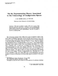
Baddeley Model L= 6 0.08 0.07 0.06 PPP variance Variance of NND

of radius r centered at y. Let Dx (r) denote the node degree of node x in a disk graph of radius r. For a homogeneous PPP, E(Dx (r)) = λπr2 . For any regular lattice process it is a staircase function of r. For an equilateral triangle lattice, it jumps by 6 for r increasing by the mean NND. For any regular lattice var(Dx (r)) = 0, and for a Poisson process var(Dx (r)) = λπr2 . var(Dx (r)) indicates the irregularity of the point process with regard to the number of points in a bounded set.

0.05 0.04 0.03 0.02 0.01

A. Some point process models 0

The Baddeley Construction [1] is a construction of a point process with the same second order characteristics as the PPP. One of the key properties of PPP is E(φ(B)) = var(φ(B)) where B is a bounded Borel set. A Baddeley process is constructed as follows. Divide the plane by randomly throwing a square grid. Let N denote the number of points in a square grid. P (N = 0) = 1 − p1 − pb ; P (N = 1) = p1 ; P (N = b) = pb , where p1 = (b − 2)/(b − 1); pb = 1/(b2 − b) and b is an integer greater than one.

Baddeley dealt with the special case of b = 10 which we generalized to any b. It is shown in [1] that E(φ(B)) = var(B) = πVB . Also k(r) = πr2 . So one cannot distinguish between a homogeneous PPP and Baddeley by observing only second order properties. In addition to these well known processes, we also use Matern hard core processes [3], and the Neyman-Scott cluster processes [3]. We have come up with other interesting point processes, defined below. Quantized Poisson processes result from quantizing homogeneous PPP in one dimension. If the area under consideration is a square of length L and one starts with initial intensity of λL, the resulting process on each line is also Poisson [5] with average density of λ. The quantized process is not a homogeneous process. Hole-0, Hole-1 processes are obtained by thinning a homogeneous PPP of intensity λp . The processes are generated as follows. • • • •

Start with a homogeneous PPP φ1 of intensity λp . Generate another homogeneous PPP φ2 of intensity µ < λp . For each x ∈ φ2 remove all the points in φ1 ∩ b(x, R). All the removed points of φ1 form the hole-0 process and the remaining points form the hole-1 process.

The intensity of the hole-1 process is given by λ exp(−µπR2 ). The intensity of the hole-0 process is given by λ(1 − exp(−µπR2 )). Lattice processes are obtained by adding d dimensional Gaussians with zero mean to the points of an integer lattice. The resulting process is stationary and is characterized by the variance of the Gaussian distribution. This may be a good model for the node placement of sensor networks if the nodes are regularly spaced with limited accuracy. Lattice processes are not homogeneous processes.

2

3

4

5

6 b

7

8

9

10

11

Fig. 1. Variance of NND for the generalized Baddeley process and homogeneous PPP, λ = 1 L(r) 1.6 1.4 1.2 1 L(r)

• •

1

0.8 Poisson Mattern, λ =1.17, h=0.3 b

0.6

Hole−0, λ =3, R=0.6,µ=0.97 p

Hole−1, λ =3,R=0.6, µ=0.36 p

0.4

Baddeley, b=10 Lattice, var=0.3 Lattice, var=0 Quantized Poisson

0.2 0

0

0.2

0.4

0.6

Fig. 2.

0.8 r

1

1.2

1.4

1.6

L-function: L(r)

B. Simulation and Results Although the homogeneous PPP is a model for CSR, it does not achieve either maximum or minimum for most of the above metrics. For example, the variance of NND which decides the link lifetime is not maximum for a stationary Poisson process. The Baddeley process which has the same second order properties as that of PPP has a larger variance for NND for some values of the parameter b as shown in Fig. 1. So on an average Baddeley network would have a lower lifetime for b > 3 (and vice-versa for b ≤ 3). In Fig. 2, L(r) is plotted for the above processes. A square of size 15 × 15 was used for the purpose of simulation. The intensity of all processes was normalized to 1. This figure indicates that Hole-0 and Hole-1 are clustered processes whereas lattice and Matern’s hard core processes [3] are regular. The Baddeley process coincides with the Poisson process as expected. Hole-0 and Hole-1 processes, which are complementary processes, are both clustered. Lattice processes with no noise and quantized Poisson processes are neither

quantities are given in [3]. Above, below and exact indicate above, below and exact match with the corresponding metric for a homogeneous PPP of the same intensity. One observes p that J(r) and E(Dx (r)) are consistent with each other. The variance of NND increases from clustering to Poisson and then reduces for regular processes.

Var(D(r)) 12 Poisson Mattern Hole−0 Hole−1 Baddeley, b=10 Baddeley, b=2 Lattice, Var=0.3 Quantized Poisson

10

Var(D(r))

8

6

4

2

0

0

Fig. 3.

Parameters Var(NND) L(r) Noise Figure p E(Dx (r)) Parameters Var(NND) L(r) Noise Figure p E(Dx (r))

0.2

0.4

0.6 r

0.8

1

1.2

Variance of node degree of disk graph: var(Dx (r))

Poisson λ=1

Matern λb = 1.175 h = 0.3

0.064 exact 1.04 exact Baddeley b = 10 0.068 exact 0.58 exact

0.039 below 0.55 below Lattice var =0.3 0.058 below 0.64 below

Hole-0 λp = 3 R = 0.6 µ = 0.97 0.06 above 2.63 above Quantized λ=1 0.11

Hole-1 λp = 3 R = 0.6 µ = 0.36 0.043 above 2.11 above

1.85

TABLE I R EGULARITY METRICS FOR DIFFERENT POINT PROCESS

strictly above or below the Poisson process. Their position depends on the scale of observation. To obtain a singleparameter metric for regularity, one can use the area under the L(r) curve to decide on the regularity of the process. In Fig. 2, the area √ under the quantized Poisson process from r = 0 to r = 1/2 λ (which is the average nearest neighbor distance of a PPP) is greater than for PPP which indicates clustering, while the area under the perfect lattice is less than that of PPP indicating regularity. In Fig. 3, the variance of the node degree for the disk graph was plotted. The Baddeley process for b = 10 is above the Poisson process whereas for b = 2 is below the Poisson process. But for the Baddeley process, E(φ(B)) = var(φ(B)) = VB . This can be explained as follows. While calculating E(Dx (r)) one conditions on the event that the node whose degree is being calculated is present, i.e., one uses the following probability in calculating expectation: P (φ(Bx (r)) = N |x ∈ φ) (Palm probability [3]). For the Poisson process, P (φ(Bx (r)) = N |x ∈ φ) = P (φ(Bx (r)) = N ), which may not be true for the Baddeley process. In Table I, the metrics in Section III were evaluated for the above processes. The estimators used for calculating these

V. C ONCLUSION In this paper, the need for defining and understanding the regularity of point process in the context of sensor networks has been motivated. Some practical metrics have been proposed and evaluated for interesting processes. These metrics only consider certain aspects of the process and are far from defining a complete regularity metric. They are important in understanding the regularity associated with a particular process and help compare other point processes with Poisson point processes with regard to their connectivity and communication properties. When deciding about the regularity of a point process, one should take into account both the irregularity in the number of points and the position of points. So it seems reasonable to combine some of the above metrics in assessing the regularity. We rate the above process in increasing order of regularity using var(Dx (r)) and variance of NND as regularity metrics. Baddeley: b = 10 < Hole-0 < Hole-1 < Quantized Poisson < Poisson < Baddeley: b = 2 < Matern hard core: h = 0.3 < Lattice: var = 0.3 < Perfect Lattice. • The Baddeley process with b = 10 has the largest variance of the node degree and also the same K(r) as the PPP. • Hole-0 and Hole-1 have a high variance of the node degree and NND. Also they are clustered processes. • The Baddeley process with b = 2 has a lower variance of node degree than PPP. • The Matern process has lower NND variance than the lattice process with noise. But the lattice process with noise has a higher variance of node degree and higher K(r). This order reverses at r = 0.6 (inhibition diameter). If the metric K(r) (area under the curve K(r)) is used, the processes would be rated as follows. Hole-1 < Hole-0 < Quantized Poisson < Poisson = Baddeley: b = 2, 10 < Lattice: var = 0.3 < Matern hard core: h = 0.3 < Perfect Lattice. R EFERENCES [1] B. W. Silverman A. J. Baddeley. A cautionary example on the use of second-order methods for analyzing point patterns. Biometrics, 40:1089– 1093, 1984. [2] D. J. Daley and D. Vere-Jones. An Introduction to the Theory of Point Processes. Springer, New York, second edition, 1998. [3] Wilfrid S. Kendall Dietrich Stoyan and Joseph Mecke. Stochastic Geometry and its Applications. Wiley, New York, 1995. [4] Peter J. Diggle. Statistical Analysis of Spatial Point Patterns. Arnold Publishers, 2003. [5] J.F.C. Kingman. Poisson Process. Oxford University Press, 1993. [6] Peter A. W. Lewis. Stochastic Point Processes: Statistical Analysis, Theory, and Applications. Wiley-Interscience, 1972. [7] Mohamed-Slim Alouini Marvin K. Simon. Digital Communication over Fading Channels. Wiley, 2000. [8] D. Stoyan. Inequalities and bounds for variances of point processes and fibre processes. Math. Operationsf. Statist., Ser. Statistics, 14:409–419, 1983.