Grupo de Dinámica Espacial (SDG–UPM) Departamento de Física Aplicada a las Ingenierías Aeronáutica y Naval
Escuela Técnica Superior de Ingenieros Aeronáuticos Universidad Politécnica de Madrid
Regularization in Astrodynamics: applications to relative motion, low-thrust missions, and orbit propagation Ph.D. Dissertation
Javier Roa Vicens Ingeniero Aeronáutico
Supervised by
Prof. Jesús Peláez Álvarez Doctor Ingeniero Aeronáutico
Madrid September 2016
Tribunal nombrado por el Sr. Rector Magfco. de la Universidad Politécnica de Madrid, el día ...... de .................... de 2016.
Presidente:
Dr. José Manuel Perales
Vocal:
Dr. Michael Efroimsky
Vocal:
Dr. Anastassios Petropoulos
Vocal:
Dr. Hodei Urrutxua
Secretario:
Dra. Ana Laverón Simavilla
Suplente:
Dr. Martín Lara Coira
Suplente:
Dr. Manuel Sanjurjo Rivo
Calificación: ...................................................
Realizado el acto de defensa y lectura de la Tesis el día 30 de septiembre de 2016 en la E.T.S.I. Aeronáuticos.
LOS VOCALES
EL PRESIDENTE
EL SECRETARIO
i
“The true voyage of discovery consists not in seeking new landscapes, but in having new eyes.” — Marcel Proust
iii
Regularization in Astrodynamics: applications to relative motion, low-thrust missions, and orbit propagation Abstract
Regularized formulations of orbital motion provide powerful tools for solving various problems in orbital mechanics, both analytically and numerically. They rely on a collection of dynamical and mathematical transformations that yields a more convenient description of the dynamics. The goal of the present thesis is to recover the foundations of regularization, to advance the theory toward practical applications, and to use this mathematical contrivance for solving three key challenges in modern astrodynamics: the dynamics of spacecraft formations, the design of low-thrust trajectories, and the high-performance numerical propagation of orbits. The introduction of a fictitious time is a typical practice when regularizing the equations of motion. This technique leads to a new theory of relative motion, called the theory of asynchronous relative motion. It improves the accuracy of the linear propagation by introducing nonlinear terms through simple dynamical mechanisms, and simplifies significantly the derivation of analytic solutions. In addition, it admits any type of orbital perturbation. The method is compact and seems well suited for its implementation in navigation filters and control laws. Universal and fully regular solutions to the relative dynamics follow naturally from this theory. They are valid for any type of reference orbit (circular, elliptic, parabolic, or hyperbolic) and are not affected by the typical singularities related to the eccentricity or inclination of the orbit. The nonlinear corrections proposed by the method are generic and can be applied to existing solutions to improve their accuracy without the need for a dedicated re-implementation. We present a novel shape-based method for preliminary design of low-thrust trajectories: the family of generalized logarithmic spirals. This new solution arises from the search for sets of orbital elements in the accelerated case. It is fully analytic and involves two conservation laws (related to the equations of the energy and angular momentum) that make the solution surprisingly similar to the Keplerian case and simplify the design process. The properties of the solution to the Keplerian Lambert problem find direct analogues in the continuous-thrust case. An analysis of the dynamical symmetries in the problem shows that the perturbing acceleration can be generalized and provides two additional families of analytic solutions: the generalized cardioids and the generalized sinusoidal spirals. As the complexity of space missions increases, more sophisticated orbit propagators are required. In order to integrate flyby trajectories more efficiently, an improved propagation scheme is presented, exploiting the geometry of Minkowski space-time. The motion of the orbital plane is decoupled from the in-plane dynamics, and the introduction of hyperbolic geometry simplifies the description of the planar motion. General considerations on the accuracy of the propagation of flyby trajectories are presented. In the context of N-body systems, we prove that regularization yields a simplified Lyapunov-like indicator that helps in assessing the validity of the numerical integration. Classical concepts arising from stability theories are extended to higher dimensions to comply with the regularized state-space. In this thesis, we present, for the first time, the gauge-generalized form of some element-based regularized formulations.
v
Regularización en Astrodinámica: aplicaciones al movimiento relativo, misiones de bajo empuje, y propagación de órbitas Resumen
Las formulaciones regularizadas del movimiento orbital son potentes herramientas para resolver diversos problemas en mecánica orbital, tanto analítica como numéricamente. Se basan en un conjunto de transformaciones físico-matemáticas que proveen una descripción más conveniente de la dinámica. El objetivo de esta tesis es recuperar las bases de la regularización, avanzar en sus fundamentos teóricos para abordar cuestiones prácticas, y emplear este artificio matemático para resolver tres retos fundamentales en la astrodinámica moderna: el movimiento de formaciones de satélites, el diseño de trayectorias de bajo empuje, y la propagación numérica de órbitas de alta precisión. Introducir un tiempo ficticio es una práctica habitual cuando se regularizan las ecuaciones del movimiento. Esta técnica da lugar a toda una nueva teoría del movimiento relativo, denominada teoría del movimiento relativo asíncrono. Mejora la precisión de la propagación al introducir términos no lineales mediante mecanismos dinámicos sencillos, y simplifica notablemente la obtención de soluciones analíticas. Además, la teoría admite cualquier tipo de perturbación. El método es compacto y adecuado para su implementación en algoritmos de navegación y leyes de control. Soluciones universales y completamente regularizadas surgen de forma natural al emplear esta teoría. Dichas soluciones son válidas para cualquier tipo de órbita de referencia (circular, elíptica, parabólica, hiperbólica) y no se ven afectadas por las típicas singularidades relacionadas con la excentricidad o la inclinación de la órbita. Las correcciones no lineales introducidas por este método son generales, y pueden aplicarse a soluciones ya existentes para mejorar su precisión sin necesidad de reimplementarlas. Se ha desarrollado un nuevo método basado en la forma para el diseño preliminar de trayectorias con bajo empuje: las espirales logarítmicas generalizadas. Esta solución surge de buscar conjuntos de elementos orbitales que permanezcan constantes en el caso acelerado. Es completamente analítica y admite dos leyes de conservación (relacionadas con las ecuaciones de la energía y el momento angular) que hacen que la solución sea sorprendentemente parecida al caso kepleriano, lo que simplifica el proceso de diseño. Las propiedades de la solución al problema de Lambert kepleriano pueden traducirse al problema con empuje continuo, donde aparecen propiedades similares. Un análisis detallado de las simetrías dinámicas del problema revela que la aceleración de perturbación puede generalizarse, dando lugar a dos familias de soluciones adicionales: los cardioides generalizados, y las espirales sinusoidales generalizadas. Conforme aumenta la complejidad de las misiones espaciales, se necesitan propagadores orbitales más avanzados. Para integrar trayectorias con flybys de forma más eficiente, se presenta un esquema de propagación mejorado que se sirve de la geometría sobre la que se fundamenta el espacio-tiempo de Minkowski. El movimiento del plano orbital se desacopla de la dinámica dentro del plano, que se ve simplificada al emplear la geometría hiperbólica. La discusión incluye consideraciones generales sobre la precisión de la propagación. En el contexto de sistemas de N-cuerpos, se demuestra que la regularización da lugar un indicador de Lyapunov simplificado que ayuda a evaluar la validez de la integración numérica. Los conceptos clásicos que se derivan de las teorías de estabilidad serán extendidos a dimensiones más altas de acuerdo con el espacio de fases regularizado. En esta tesis se presenta, por primera vez, la generalización gauge de ciertas formulaciones regularizadas basadas en elementos.
vii
Acknowledgments Gracias, Jesús. I feel like I would never say this enough. I first contacted Prof. Jesús Peláez by chance back in 2012 (referred by Prof. Rafael Ramis, to whom I will always be grateful), and I completed my master’s thesis under his supervision. Not only did he teach me all I know about astrodynamics, but I also owe him my passion for orbital mechanics. That is why I did not hesitate about pursuing a Ph.D. under his supervision. This was to become one of the best decisions of my life, and I want to thank him for accepting me as his student. He has truly been a maestro, in all its Spanish meaning, more than a mere teacher. If this were not enough, he was also who arranged my trip to the Jet Propulsion Laboratory during the second year of my doctorate (I still remember that first email he sent me on August 7, 2014). Then, he gave me his full support when I suggested the possibility of finishing what remained of my Ph.D. from the U.S., and agreed to supervise my work remotely. I will miss those Skype calls. Thanks to him I am living my dream, and I just hope that I will be able to repay him, somehow, in the future. Gracias, Juan. If it were not for Dr. Juan Senent, I would have never come to JPL in the first place. And for that I am indebted to him. He convinced me of the importance of solving actual problems in engineering, as opposed to just developing abstract methods, and helped me complete this thesis with realworld applications. Moreover, he motivated me to look into continuous-thrust trajectories, which resulted in the new analytic solution and design strategy presented in Chapters 9–12. I could not have felt more welcomed: in fact, have I had a different advisor, I may not have considered extending my stay. Gracias, Fernando. I feel truly lucky to have met Fernando Abilleira while at JPL. Specially because I met him almost by chance. He had no obligation toward me: still, he became a constant support both in the professional and personal sides. For me, he has been an example of motivation and perseverance, and he always found the right encouraging words for the not-so-good times. He welcomed Marta and me into his family, and I will never forget that. Thanks to him California felt a little more like home. I feel fortunate that this adventure has just started. But I am sure that I would not have made it without his help. I want to thank Dr. Michael Efroimsky for his selfless help and guidance. To me, he has been the perfect example of how a researcher should be: willing to collaborate, to discuss exciting concepts, and always open to new ideas. He referred me to the gauge freedom in celestial mechanics, a topic that I found fascinating from the first time I looked into it. In addition, he read this dissertation thoroughly and made very valuable suggestions. A good part of this thesis focuses on the numerical integration of orbits. And I owe almost all I know about this subject to Dr. Hodei Urrutxua. He was always there to answer my questions, providing a detailed explanation. I really enjoyed our conversations, and I look forward to working together in so many projects that we discussed. I would also like to thank Dr. Sebastien Le Maistre for his company, for sharing his office with me, and for all he taught me about planetary science. The trailer is not the same without him… Dr. Anatoliy Ivantsov was kind enough to share his expertise on rotation models with me. Let me also thank Jordi Paredes for transmitting me his resolve, and for showing me that it pays to persevere. Dr. Claudio Bombardelli got me involved in very exciting projects that helped me learn many things, and he taught me many others. His door was always open to me, and I cannot wait to recover some of the ideas that we discussed and to collaborate in the future. Gracias, Claudio. Dr. Anastassios Petropoulos and Dr. Nitin Arora’s help was invaluable when developing the continuous-thrust theory. Many ideas came up during our meetings. I would like to thank Dr. Vladimir Martinuşi for our conversations about relative motion, which contributed to improving the present work. Similarly, I would like to thank Dr. Giulio Baù for many interesting debates about orbit propagation, and I hope that we will find the time in the future to finish our projects. I had a great time discussing historical references with Dr. Aaron Rosengren. I thank Carolina Silva, Kim Jackson, Arpine Margallan, and Claudia Tobar for their assistance while at JPL. I was lucky enough to participate in the Caltech Space Challenge with Team Voyager, and to meet so interesting people. I am also grateful to Prof. Carlos Blanco-Pérez for our exciting conversations. I can only be grateful to the people I worked with in Madrid: to Juan Luis Gonzalo, for all his help with coding, and everything related to computers; to Dr. Manuel Sanjurjo and David Morante, for their work on trajectory optimization using generalized logarithmic spirals; to Davide Amato and Javier Hernando,
ix
for their help when facing the doctoral courses; to Mari Carmen Velasco, María Rosa García, María Jesús de Andrés, Pablo Velasco and Silvia Muñoz, for solving each and every administrative problem I had. And to Ana, for welcoming me every morning with a smile. I can say that this Ph.D. would not have been possible without their constant assistance. Many people helped me in one way or the other during these years. Dr. Rodney Anderson referred me to very interesting problems involving periodic orbits, and helped me prepare several proposals. I would also like to thank Dr. Jon Sims, Dr. Roby Wilson, Dr. Ralph Roncoli, and Dr. Joe Guinn for their patience and council, and I hope did not get too persistent. This Acknowledgments section would not be complete without thanking Dr. Ryan Park, Dr. Paul Chodas, and Dr. Steve Chesley for believing in me and for offering me the opportunity to work with them. Dr. Mar Vaquero was a constant support to me, and I thank her for referring me to this group in the first place. I would like to thank Prof. Jeremy Kasdin for inviting me to Princeton, and Prof. Simone D’Amico for his time and consideration; I hope we will have the chance to work on some of the ideas we discussed. I am deeply grateful to all the members of the committee evaluating this thesis (Prof. José Manuel Perales, Dr. Michael Efroimsky, Dr. Anastassios Petropoulos, Dr. Hodei Urrutxua, Prof. Ana Laverón, Dr. Martín Lara, and Dr. Manuel Sanjurjo) and also to Prof. Terry Alfriend and Prof. Massimiliano Vasile for reviewing this manuscript in great detail. This past year I have asked for a lot of recommendation letters, for which I would like to acknowledge Dr. Martín Lara, Dr. Martin Ozimek, Dr. Johan Knapen (also for hosting me at the Instituto de Astrofísica de Canarias in 2013), Prof. Ryan Russell, and Prof. Roberto Furfaro. Dr. Ozimek also made valuable contributions to the low-thrust work, and Dr. Lara helped me with various proposals. I could not forget that Prof. Peláez, Dr. Senent, F. Abilleira, and Dr. Efroimsky acted as references many times too. My Ph.D. was possible thanks to the financial support of Obra Social “La Caixa”. I am grateful not only for the doctoral fellowship, but for all the help that I received, the activities of the society, the networking events, etc. I thank Ainhoa Martín, Anna Mauri, María Inmaculada Jiménez, Elisabeth Linero, and the rest of the team at Fundación “La Caixa”. I am also grateful to Prof. Carmina Crusafón for including me in the board. So many emotions and memories come to my mind when thanking my parents. They have always been there for me, specially in the most stressful moments. Always supportive, always understanding my dedication, and always putting my needs before theirs. I hope that they realize that all I achieved was because of them, and that they are proud of who I have become. With their example and dedicated lives they taught me the most important lessons one can learn. They are the best models I can think of. In my brother I have always found the right piece of advice, the perfect words of encouragement, and I thank for him for his patience and for teaching me with his brilliant example. My sister has been able to transmit her illusions to me, her will for living, and her constant joy. She has the gift of cheering up every situation, a gift that was most valuable in the difficult moments. Einstein once said that love is power, because it multiplies the best we have. And this is his only theory that I have been able to prove, or at least to experience myself. And for that I thank Marta. She has always been there, she has been my constant support, encouraging me to keep going. She made so many sacrifices for me… It has not been an easy path. But, precisely because it was hard, we can now look back happily and enjoy the fact that we finally made it. With time one realizes that the best of achieving your goals is to have someone to share them with. I could not have been luckier. And this thesis is my gift to you. Gracias, Marta.
Javier Roa Vicens Pasadena, CA, August 2016
x
Dissertation Overview This dissertation consists in two parts. The first part focuses on the theoretical aspects of regularization, and the second part exploits the properties and advantages of regularized formulations to tackle different problems in astrodynamics. When reading a dissertation for the first time, it is often hard to know what sections are reviews of existing work, and what sections introduce new and truly original material. For this reason, the following lines describe briefly the contents of each chapter, stating clearly where the new concepts and results are presented. Chapter 1: this is the introduction to the thesis. It discusses the relevance of the three problems that will be addressed in the second part of the dissertation: spacecraft relative motion, low-thrust mission design, and orbit propagation. Chapter 2: the second chapter is devoted to the theory of regularization. It starts by justifying why regularization is useful, and revisits various methods and techniques that improve the description of orbital motion. This chapter introduces several concepts that will be recovered throughout the dissertation. Chapter 3: a completely new theory of stability is presented in this chapter, based on the topology of Kustaanheimo-Stiefel (KS) space. It leads to a novel Lyapunov indicator. The second part of the chapter provides the elements attached to KS space with an innovative geometric interpretation. Finally, the gauge-generalized form of the equations of motion in this formalism is derived for the first time. Chapter 4: the first part of this chapter is a review of the Dromo formulation, a special-perturbation method. The second part presents new results related to the singularity of Dromo, and the gaugegeneralized version of the equations of motion. Chapter 5: the chapter presents a novel propagation method for hyperbolic orbits, based on the geometry of Minkowski space-time and recovering the dynamical structure of the Dromo propagator. The result is a more stable integration scheme, which is more accurate because of not being affected by periapsis passage. Chapter 6: this chapter explains the structure of the high-fidelity orbit propagator developed during this doctoral work. The force models are discussed in detail. The main goal of the software is to compare the performance of various numerical propagation methods. Chapter 7: this is the first chapter in the second part of the dissertation, and focuses on spacecraft relative motion. After an introduction to the problem, the theory of asynchronous relative motion is presented. It is a novel concept that approaches the problem from the perspective of regularization. It improves the accuracy of the purely linear solution without complicating the algorithm significantly. This new theory can be applied in many other scenarios apart from relative motion (as long as they involve the variational equations of motion) and admits any source of perturbation. Chapter 8: making use of the theory of asynchronous relative motion, this chapter models the relative dynamics using various regularized formulations. The result is a fully universal and regular solution, more accurate than the linear one and valid for any type of orbit. Chapter 9: a new analytic solution with continuous thrust is derived: the generalized logarithmic spirals. This new family of curves has interesting properties for preliminary design of low-thrust missions. There are two integrals of motion that make the solution very similar to the Keplerian case. The thrust decreases with the square of the radial distance and it is directed along the velocity vector. Chapter 10: using the new analytic solution presented in the previous chapter, Chapter 10 solves Lambert’s problem with continuous thrust. The versatility of the solution is improved by introducing a control parameter. It affects both the magnitude and direction of the thrust vector: it is no longer tangential. The properties of the ballistic Lambert problem are then translated to the continuous-thrust case. Examples of application to mission design can also be found. Chapter 11: advancing on the solution to Lambert’s problem, in Chapter 11 the reader will find a new design strategy for generating preliminary continuous-thrust transfer solutions, including examples. Al-
xi
though the original solution is planar, a fully three-dimensional approach is derived in this chapter. In Appendix G the potential of Seiffert’s spherical spirals for mission design is explored. Chapter 12: in this chapter, it is demonstrated that the family of generalized logarithmic spirals can be generalized by adding an extra degree of freedom to the perturbing acceleration in order to yield new families of orbits. The symmetries of Kepler’s problem are exploited to render integrals of motion with continuous thrust. Keplerian orbits and generalized logarithmic spirals appear naturally as particular instances of this new and more general integrable system. Chapter 13: the final chapter includes the conclusions to the thesis and suggests future lines of research. The paper based on Chapter 7 won the Best Paper Award at the 25th AAS/AIAA Space Flight Mechanics Meeting in Williamsburg, VA, January 11-15, 2015. The next section includes the complete list of publications based on the present dissertation.
xii
xiii
List of Publications During my doctoral studies I have been involved in the preparation of the following research papers, and I presented several others in international conferences:
Publications in Journals of the JCR 1. Roa, J. (2016): “Nonconservative extension of Keplerian integrals and a new class of integrable system,” Monthly Notices of the Royal Astronomical Society. Available online, doi: 10.1093/mnras/stw2209. 2. Roa, J. and Peláez, J. (2016): “The theory of asynchronous relative motion I: Time transformations and nonlinear terms,” Celestial Mechanics and Dynamical Astronomy. Available online, doi: 10.1007/s10569-016-9728-6. 3. Roa, J. and Peláez, J. (2016): “The theory of asynchronous relative motion II: Universal and regular solutions,” Celestial Mechanics and Dynamical Astronomy. Available online, doi: 10.1007/s10569-016-9730-z. 4. Roa, J., Peláez, J. and Senent, J. (2016): “New analytic solution with continuous thrust: generalized logarithmic spirals,” Journal of Guidance, Control and Dynamics, Vol. 39, No. 10, pp. 2336–2351. doi: 10.2514/1.G000341. 5. Roa, J., Peláez, J. and Senent, J. (2016): “Spiral Lambert’s problem,” Journal of Guidance, Control and Dynamics, Vol. 39, No. 10, pp. 2250–2263. doi: 10.2514/1.G000342. 6. Bombardelli, C., Gonzalo, J.L. and Roa, J. (2016): “Approximate solution of nonlinear circular orbit relative motion in curvilinear coordinates,” Celestial Mechanics and Dynamical Astronomy. Available online, doi: 10.2514/1.G000341. 7. Roa, J., Urrutxua, H., and Peláez, J. (2016): “Stability and chaos in Kustaanheimo-Stiefel space induced by the Hopf fibration,” Monthly Notices of the Royal Astronomical Society, Vol. 459, No. 3, pp. 2444–2454. doi: 10.1093/mnras/stw780. 8. Roa, J. and Peláez, J. (2015): “Orbit propagation in Minkowskian geometry,” Celestial Mechanics and Dynamical Astronomy, (123) 13–43. doi: 10.1007/s10569-015-9627-2. 9. Roa, J., Sanjurjo-Rivo, M. and Peláez, J. (2015): “Singularities in Dromo formulation. Analysis of deep flybys,” Advances in Space Research, Vol. 56, No. 3, pp. 569–581. doi: 10.1016/j.asr.2015.03.019. 10. Roa, J. and Peláez, J. (2015): “Frozen-anomaly transformation for the elliptic rendez-vous problem,” Celestial Mechanics and Dynamical Astronomy, Vol. 121, No. 1, pp. 61–81. doi: 10.1007/s10569-0149585-0. 11. Knapen, J.H., Erroz-Ferrer, S., Roa, J., Bakos, J., Cisternas, M., Leaman, R. and Szymanek, N. (2014): “Optical imaging of galaxies from the Spitzer Survey of Stellar Structure in Galaxies.” Astronomy and Astrophysics, Vol. 569, A91. doi: 10.1051/0004-6361/201322954
Conference Proceedings 1. Roa, J. and Peláez, J.: “Spiral Lambert’s problem with generalized logarithmic spirals,” 26th AAS/AIAA Space Flight Mechanics Meeting in Napa, CA, USA. February 14-18, 2016. AAS 16-316. 2. Roa, J. and Peláez, J.: “Introducing a degree of freedom in the family of generalized logarithmic spirals,” 26th AAS/AIAA Space Flight Mechanics Meeting in Napa, CA, USA. February 14-18, 2016. AAS 16-317. 3. Roa, J. and Peláez, J.: “Three-dimensional generalized logarithmic spirals,” 26th AAS/AIAA Space Flight Mechanics Meeting in Napa, CA, USA. February 14-18, 2016. AAS 16-323. xiv
4. Urrutxua, H., Roa, J., Gonzalo, J. L., Peláez, J. and Bombardelli, C.: “Quantification of the Performance of Numerical Orbit Propagators,” 26th AAS/AIAA Space Flight Mechanics Meeting in Napa, CA, USA. February 14-18, 2016. AAS 16-351. 5. Bombardelli, C., Roa, J. and Gonzalo, J.L.: “Approximate Analytical Solution of the Multiple Revolution Lambert’s Problem,” 26th AAS/AIAA Space Flight Mechanics Meeting in Napa, CA, USA. February 14-18, 2016. AAS 16-212. 6. Roa, J. and Peláez, J.: “Generalized logarithmic spirals for low-thrust trajectory design,” 2015 AAS/AIAA Astrodynamics Specialist Conference in Vail, CO, USA. August 9-13, 2015. AAS 15-729. 7. Roa, J. and Peláez, J.: “Efficient trajectory propagation for orbit determination problems,” 2015 AAS/AIAA Astrodynamics Specialist Conference in Vail, CO, USA. August 9-13, 2015. AAS 15-730. 8. Bombardelli, C., Gonzalo, J.L. and Roa, J.: “Compact solution of circular orbit relative motion in curvilinear coordinates,” 2015 AAS/AIAA Astrodynamics Specialist Conference in Vail, CO, USA. August 9-13, 2015. AAS 15-661. 9. Roa, J. and Peláez, J.: “Regularized formulations in relative motion,” 25th AAS/AIAA Space Flight Mechanics Meeting in Williamsburg, VA, USA. January 11-15, 2015. AAS 15-210. 10. Roa, J., Gómez-Mora, J.I. and Peláez, J.: “Error propagation in relative motion,” 25th AAS/AIAA Space Flight Mechanics Meeting in Williamsburg, VA, USA. January 11-15, 2015. AAS 15-272. 11. Roa, J. and Peláez, J.: “Orbit propagation in Minkowskian geometry,” 25th AAS/AIAA Space Flight Mechanics Meeting in Williamsburg, VA, USA. January 11-15, 2015. AAS 15-209. 12. Roa, J., Sanjurjo-Rivo, M. and Peláez, J.: “A nonsingular Dromo formulation,” 2nd KEPASSA Workshop, La Rioja, Spain. April 14-17, 2014. 13. Roa, J. and Peláez, J.: “The elliptic rendezvous problem in Dromo formulation,” 24th AAS/AIAA Space Flight Mechanics Meeting in Santa Fe, NM, USA. January 26-30, 2014. AAS 14-382.
Non-Refereed Publications 1. Roa, J. and Handmer, C. (2015): “Quantifying hazards: asteroid disruption in lunar distant retrograde orbits,” arXiv preprint arXiv:1505.03800.
xv
Contents Abstract
v
Resumen
vii
Acknowledgments
ix
Dissertation Overview
xi
List of Publications
xiii
Contents
xvii
1
Introduction. Current challenges in space exploration 1.1 Accessible space . . . . . . . . . . . . . . . . . 1.2 Distributed space systems . . . . . . . . . . . . 1.3 Efficient orbit transfers . . . . . . . . . . . . . 1.4 Orbit propagation . . . . . . . . . . . . . . . . 1.5 The aim of the present thesis . . . . . . . . . .
I
Regularization
2
Theoretical Aspects of Regularization 2.1 Why bother? . . . . . . . . . . . . . . 2.2 The Sundman transformation . . . . . . 2.3 Stabilization of the equations of motion 2.4 Linearization . . . . . . . . . . . . . . 2.5 Sets of orbital elements . . . . . . . . . 2.6 Canonical transformations . . . . . . . 2.7 Gauge-freedom in celestial mechanics . . 2.8 Conclusions . . . . . . . . . . . . . . .
3
. . . . .
. . . . .
. . . . .
. . . . .
. . . . .
. . . . .
. . . . .
. . . . .
. . . . .
. . . . .
. . . . .
. . . . .
. . . . .
. . . . .
. . . . .
. . . . .
. . . . .
. . . . .
. . . . .
. . . . .
. . . . .
. . . . .
. . . . .
. . . . .
. . . . .
. . . . .
. . . . .
. . . . .
. . . . .
. . . . .
. . . . .
. . . . .
. . . . .
. . . . .
. . . . .
1 1 2 3 4 5
7 . . . . . . . .
. . . . . . . .
. . . . . . . .
. . . . . . . .
. . . . . . . .
. . . . . . . .
. . . . . . . .
. . . . . . . .
The Kustaanheimo-Stiefel space and the Hopf fibration
. . . . . . . .
. . . . . . . .
. . . . . . . .
. . . . . . . .
. . . . . . . .
. . . . . . . .
. . . . . . . .
. . . . . . . .
. . . . . . . .
. . . . . . . .
. . . . . . . .
. . . . . . . .
. . . . . . . .
. . . . . . . .
. . . . . . . .
. . . . . . . .
. . . . . . . .
. . . . . . . .
. . . . . . . .
. . . . . . . .
. . . . . . . .
. . . . . . . .
. . . . . . . .
. . . . . . . .
. . . . . . . .
. . . . . . . .
. . . . . . . .
. . . . . . . .
. . . . . . . .
. . . . . . . .
. . . . . . . .
9 10 11 14 15 18 20 21 23 25
xvii
3.1 3.2 3.3 3.4 3.5 3.6 3.7 3.8 4
5
6
The need for an extra dimension: fibrations of hyperspheres The KS transformation as a Hopf map . . . . . . . . . . . Stability in KS space . . . . . . . . . . . . . . . . . . . . . Order and chaos . . . . . . . . . . . . . . . . . . . . . . . Topological stability in N -body problems . . . . . . . . . . Gauge-generalized elements in KS space . . . . . . . . . . . Orthogonal bases . . . . . . . . . . . . . . . . . . . . . . Conclusions . . . . . . . . . . . . . . . . . . . . . . . . .
. . . . . . . .
. . . . . . . .
. . . . . . . .
. . . . . . . .
. . . . . . . .
. . . . . . . .
. . . . . . . .
. . . . . . . .
. . . . . . . .
. . . . . . . .
. . . . . . . .
. . . . . . . .
. . . . . . . .
. . . . . . . .
. . . . . . . .
. . . . . . . .
. . . . . . . .
. . . . . . . .
. . . . . . . .
. . . . . . . .
. . . . . . . .
. . . . . . . .
. . . . . . . .
. . . . . . . .
. . . . . . . .
. . . . . . . .
. . . . . . . .
. . . . . . . .
. . . . . . . .
26 27 30 33 34 36 40 41
The Dromo formulation 4.1 Hansen ideal frames . . . . . . . . . . . . . . . . . . 4.2 Dromo . . . . . . . . . . . . . . . . . . . . . . . . 4.3 Improved performance . . . . . . . . . . . . . . . . 4.4 Variational equations and the noncanonicity of Dromo 4.5 Gauge-generalized Dromo formulation . . . . . . . . 4.6 Singularities . . . . . . . . . . . . . . . . . . . . . . 4.7 Modified Dromo equations . . . . . . . . . . . . . . 4.8 Numerical experiments . . . . . . . . . . . . . . . . 4.9 Conclusions . . . . . . . . . . . . . . . . . . . . . .
. . . . . . . . .
. . . . . . . . .
. . . . . . . . .
. . . . . . . . .
. . . . . . . . .
. . . . . . . . .
. . . . . . . . .
. . . . . . . . .
. . . . . . . . .
. . . . . . . . .
. . . . . . . . .
. . . . . . . . .
. . . . . . . . .
. . . . . . . . .
. . . . . . . . .
. . . . . . . . .
. . . . . . . . .
. . . . . . . . .
. . . . . . . . .
. . . . . . . . .
. . . . . . . . .
. . . . . . . . .
. . . . . . . . .
. . . . . . . . .
. . . . . . . . .
. . . . . . . . .
. . . . . . . . .
. . . . . . . . .
. . . . . . . . .
. . . . . . . . .
. . . . . . . . .
. . . . . . . . .
43 44 44 47 48 49 49 50 51 53
Orbit propagation in Minkowskian geometry 5.1 Orbital motion . . . . . . . . . . . . . . . 5.2 Hyperbolic rotations and the Lorentz group 5.3 Variation of Parameters . . . . . . . . . . . 5.4 Orbital plane dynamics . . . . . . . . . . . 5.5 Time element . . . . . . . . . . . . . . . . 5.6 Numerical evaluation . . . . . . . . . . . . 5.7 Conclusions . . . . . . . . . . . . . . . . .
. . . . . . .
. . . . . . .
. . . . . . .
. . . . . . .
. . . . . . .
. . . . . . .
. . . . . . .
. . . . . . .
. . . . . . .
. . . . . . .
. . . . . . .
. . . . . . .
. . . . . . .
. . . . . . .
. . . . . . .
. . . . . . .
. . . . . . .
. . . . . . .
. . . . . . .
. . . . . . .
. . . . . . .
. . . . . . .
. . . . . . .
. . . . . . .
. . . . . . .
. . . . . . .
. . . . . . .
. . . . . . .
. . . . . . .
. . . . . . .
. . . . . . .
. . . . . . .
55 56 58 59 61 62 63 66
. . . .
. . . .
. . . .
. . . .
. . . .
. . . .
. . . .
. . . .
. . . .
. . . .
. . . .
. . . .
. . . .
. . . .
. . . .
. . . .
. . . .
. . . .
. . . .
. . . .
69 70 72 76 79
. . . . . . .
. . . . . . .
. . . . . . .
. . . . . . .
. . . . . . .
PERFORM: Performance Evaluation of Regularized Formulations of Orbital Motion
6.1 6.2 6.3 6.4
Implementation . . . . . . . . . . . . PERFORM as a high-fidelity propagator Evaluating the performance . . . . . . Conclusions . . . . . . . . . . . . . .
. . . .
. . . .
. . . .
. . . .
. . . .
. . . .
. . . .
. . . .
. . . .
. . . .
. . . .
. . . .
. . . .
. . . .
. . . .
. . . .
. . . .
. . . .
. . . .
. . . .
II Applications 7
8
9
The theory of asynchronous relative motion 7.1 Definition of the problem . . . . . . . 7.2 Synchronism in relative motion . . . . 7.3 Generalizing the transformation . . . . 7.4 The circular case . . . . . . . . . . . . 7.5 Numerical evaluation . . . . . . . . . 7.6 Conclusions . . . . . . . . . . . . . .
83 . . . . . .
. . . . . .
. . . . . .
. . . . . .
. . . . . .
. . . . . .
. . . . . .
. . . . . .
. . . . . .
. . . . . .
. . . . . .
. . . . . .
. . . . . .
. . . . . .
. . . . . .
. . . . . .
. . . . . .
. . . . . .
. . . . . .
. . . . . .
. . . . . .
. . . . . .
. . . . . .
. . . . . .
. . . . . .
. . . . . .
. . . . . .
. . . . . .
. . . . . .
. . . . . .
. . . . . .
. . . . . .
. . . . . .
. . . . . .
. . . . . .
85 86 87 91 94 96 98
Regularization in relative motion 8.1 Relative motion in Dromo variables . . . . . . . . 8.2 Relative motion in Sperling-Burdet variables . . . 8.3 Relative motion in Kustaanheimo-Stiefel variables 8.4 On the fictitious time . . . . . . . . . . . . . . . 8.5 Numerical examples . . . . . . . . . . . . . . . . 8.6 Generic propagation of the variational equations . 8.7 Conclusions . . . . . . . . . . . . . . . . . . . .
. . . . . . .
. . . . . . .
. . . . . . .
. . . . . . .
. . . . . . .
. . . . . . .
. . . . . . .
. . . . . . .
. . . . . . .
. . . . . . .
. . . . . . .
. . . . . . .
. . . . . . .
. . . . . . .
. . . . . . .
. . . . . . .
. . . . . . .
. . . . . . .
. . . . . . .
. . . . . . .
. . . . . . .
. . . . . . .
. . . . . . .
. . . . . . .
. . . . . . .
. . . . . . .
. . . . . . .
. . . . . . .
. . . . . . .
. . . . . . .
. . . . . . .
. . . . . . .
. . . . . . .
. . . . . . .
101 102 103 105 106 107 108 112
Generalized logarithmic spirals: a new analytic solution with continuous thrust 9.1 The Equations of Motion. First Integrals . . . . . . . . . . . . . . . . . 9.2 Elliptic Spirals (K1 < 0) . . . . . . . . . . . . . . . . . . . . . . . . . . 9.3 Parabolic Spirals (K1 = 0) . . . . . . . . . . . . . . . . . . . . . . . . . 9.4 Hyperbolic Spirals (K1 > 0) . . . . . . . . . . . . . . . . . . . . . . . .
. . . .
. . . .
. . . .
. . . .
. . . .
. . . .
. . . .
. . . .
. . . .
. . . .
. . . .
. . . .
. . . .
. . . .
. . . .
. . . .
. . . .
. . . .
. . . .
. . . .
. . . .
. . . .
113 114 119 120 121
. . . . . .
. . . . . .
. . . . . .
. . . . . .
. . . . . .
xviii
9.5 9.6 9.7 9.8 9.9 9.10
Summary . . . . . . . . . Osculating Elements . . . . In-Orbit Departure Point . Practical Considerations . . Continuity of the solution Conclusions . . . . . . . .
. . . . . .
. . . . . .
. . . . . .
. . . . . .
. . . . . .
. . . . . .
. . . . . .
. . . . . .
. . . . . .
. . . . . .
. . . . . .
. . . . . .
. . . . . .
. . . . . .
. . . . . .
. . . . . .
. . . . . .
. . . . . .
. . . . . .
. . . . . .
. . . . . .
. . . . . .
. . . . . .
. . . . . .
. . . . . .
. . . . . .
. . . . . .
. . . . . .
. . . . . .
. . . . . .
. . . . . .
. . . . . .
. . . . . .
. . . . . .
. . . . . .
. . . . . .
. . . . . .
. . . . . .
. . . . . .
. . . . . .
. . . . . .
. . . . . .
. . . . . .
. . . . . .
. . . . . .
. . . . . .
125 125 126 128 128 129
10 Lambert’s problem with generalized logarithmic spirals 10.1 Introduction to Lambert’s problem . . . . . . . 10.2 Controlled generalized logarithmic spirals . . . . 10.3 The two-point boundary-value problem . . . . 10.4 Fixing the time of flight . . . . . . . . . . . . . 10.5 Repetitive transfers . . . . . . . . . . . . . . . 10.6 Evaluating the performance . . . . . . . . . . . 10.7 Additional properties . . . . . . . . . . . . . . 10.8 Additional dynamical constraints . . . . . . . . 10.9 Conclusions . . . . . . . . . . . . . . . . . . .
. . . . . . . . .
. . . . . . . . .
. . . . . . . . .
. . . . . . . . .
. . . . . . . . .
. . . . . . . . .
. . . . . . . . .
. . . . . . . . .
. . . . . . . . .
. . . . . . . . .
. . . . . . . . .
. . . . . . . . .
. . . . . . . . .
. . . . . . . . .
. . . . . . . . .
. . . . . . . . .
. . . . . . . . .
. . . . . . . . .
. . . . . . . . .
. . . . . . . . .
. . . . . . . . .
. . . . . . . . .
. . . . . . . . .
. . . . . . . . .
. . . . . . . . .
. . . . . . . . .
. . . . . . . . .
. . . . . . . . .
. . . . . . . . .
. . . . . . . . .
. . . . . . . . .
. . . . . . . . .
. . . . . . . . .
. . . . . . . . .
. . . . . . . . .
131 131 132 134 138 139 140 140 141 143
11 Low-thrust trajectory design with extended generalized logarithmic spirals 11.1 Orbit transfers . . . . . . . . . . . . . . . . . . . . . . . . . . . . 11.2 Periodic orbits . . . . . . . . . . . . . . . . . . . . . . . . . . . . 11.3 Multinode transfers . . . . . . . . . . . . . . . . . . . . . . . . . 11.4 Three-dimensional motion . . . . . . . . . . . . . . . . . . . . . 11.5 Applications . . . . . . . . . . . . . . . . . . . . . . . . . . . . . 11.6 Conclusions . . . . . . . . . . . . . . . . . . . . . . . . . . . . .
. . . . . .
. . . . . .
. . . . . .
. . . . . .
. . . . . .
. . . . . .
. . . . . .
. . . . . .
. . . . . .
. . . . . .
. . . . . .
. . . . . .
. . . . . .
. . . . . .
. . . . . .
. . . . . .
. . . . . .
. . . . . .
. . . . . .
. . . . . .
. . . . . .
. . . . . .
. . . . . .
. . . . . .
. . . . . .
145 145 150 151 152 156 159
12 Nonconservative extension of Keplerian integrals and new families of orbits 12.1 The role of first integrals . . . . . . . . . . . . . . . . . . . . . . . 12.2 Dynamics . . . . . . . . . . . . . . . . . . . . . . . . . . . . . . . 12.3 Case γ = 1: conic sections . . . . . . . . . . . . . . . . . . . . . . . 12.4 Case γ = 2: generalized logarithmic spirals . . . . . . . . . . . . . . 12.5 Case γ = 3: generalized cardioids . . . . . . . . . . . . . . . . . . . 12.6 Case γ = 4: generalized sinusoidal spirals . . . . . . . . . . . . . . . 12.7 Summary . . . . . . . . . . . . . . . . . . . . . . . . . . . . . . . 12.8 Unified solution in Weierstrassian formalism . . . . . . . . . . . . . 12.9 Physical discussion of the solutions . . . . . . . . . . . . . . . . . . 12.10 Conclusions . . . . . . . . . . . . . . . . . . . . . . . . . . . . . .
. . . . . . . . . .
. . . . . . . . . .
. . . . . . . . . .
. . . . . . . . . .
. . . . . . . . . .
. . . . . . . . . .
. . . . . . . . . .
. . . . . . . . . .
. . . . . . . . . .
. . . . . . . . . .
. . . . . . . . . .
. . . . . . . . . .
. . . . . . . . . .
. . . . . . . . . .
. . . . . . . . . .
. . . . . . . . . .
. . . . . . . . . .
. . . . . . . . . .
. . . . . . . . . .
. . . . . . . . . .
. . . . . . . . . .
. . . . . . . . . .
. . . . . . . . . .
. . . . . . . . . .
161 161 163 166 166 166 169 172 172 173 175
13 Conclusions to the thesis 177 13.1 Outlook and advances . . . . . . . . . . . . . . . . . . . . . . . . . . . . . . . . . . . . . . . . . . . . . . . . . 177 13.2 Future work . . . . . . . . . . . . . . . . . . . . . . . . . . . . . . . . . . . . . . . . . . . . . . . . . . . . . . 178
Appendices
180
A Hypercomplex numbers 183 A.1 Complex and hyperbolic numbers . . . . . . . . . . . . . . . . . . . . . . . . . . . . . . . . . . . . . . . . . . . 184 A.2 Quaternions . . . . . . . . . . . . . . . . . . . . . . . . . . . . . . . . . . . . . . . . . . . . . . . . . . . . . . 185 B Formulations in PERFORM
187
C Stumpff functions
189
D Inverse transformations D.1 Inverse transformations in equinoctial variables . . . . . . . . . . . . . . . . . . . . . . . . . . . . . . . . . . . . D.2 Cartesian to Dromo . . . . . . . . . . . . . . . . . . . . . . . . . . . . . . . . . . . . . . . . . . . . . . . . . . D.3 Linear form of the Hopf fibration . . . . . . . . . . . . . . . . . . . . . . . . . . . . . . . . . . . . . . . . . . .
193 193 194 195
E Elliptic integrals and elliptic functions 197 E.1 Properties and practical relations . . . . . . . . . . . . . . . . . . . . . . . . . . . . . . . . . . . . . . . . . . . 198 xix
E.2 E.3 E.4
Implementations . . . . . . . . . . . . . . . . . . . . . . . . . . . . . . . . . . . . . . . . . . . . . . . . . . . 198 Jacobi elliptic functions . . . . . . . . . . . . . . . . . . . . . . . . . . . . . . . . . . . . . . . . . . . . . . . . 199 Weierstrass elliptic functions . . . . . . . . . . . . . . . . . . . . . . . . . . . . . . . . . . . . . . . . . . . . . 199
F Controlled generalized logarithmic spirals F.1 Elliptic spirals . . . . . . . . . . . F.2 Parabolic spirals . . . . . . . . . . F.3 Hyperbolic spirals . . . . . . . . . F.4 Osculating elements . . . . . . . .
. . . .
. . . .
. . . .
. . . .
. . . .
. . . .
. . . .
. . . .
. . . .
. . . .
. . . .
. . . .
. . . .
. . . .
. . . .
. . . .
. . . .
. . . .
. . . .
. . . .
. . . .
. . . .
. . . .
. . . .
. . . .
. . . .
. . . .
. . . .
. . . .
. . . .
. . . .
. . . .
. . . .
. . . .
. . . .
. . . .
. . . .
. . . .
. . . .
. . . .
201 202 203 203 205
G Dynamics in Seiffert’s spherical spirals G.1 Dynamics . . . . . . . . . . . . . . . . G.2 The geometry of Seiffert’s spherical spirals G.3 Groundtracks . . . . . . . . . . . . . . G.4 Relative motion between Seiffert’s spirals G.5 The significance of Seiffert’s spirals . . .
. . . . .
. . . . .
. . . . .
. . . . .
. . . . .
. . . . .
. . . . .
. . . . .
. . . . .
. . . . .
. . . . .
. . . . .
. . . . .
. . . . .
. . . . .
. . . . .
. . . . .
. . . . .
. . . . .
. . . . .
. . . . .
. . . . .
. . . . .
. . . . .
. . . . .
. . . . .
. . . . .
. . . . .
. . . . .
. . . . .
. . . . .
. . . . .
. . . . .
. . . . .
. . . . .
. . . . .
. . . . .
. . . . .
. . . . .
207 207 210 210 211 212
. . . .
. . . .
List of Figures
213
References
217
Index
229
xx
“I would like to die on Mars. Just not on impact.” — Elon Musk
1
Introduction. Current challenges in space exploration
S
pace programs have undergone profound changes, from economic restructuring to the implementation of novel mission architectures. During the Cold War, space projects enjoyed an apparently unlimited funding that led to unprecedented technical and scientific breakthroughs in just a few years. In fact, between 1958 and 1966, when it reached its historical maximum, the budget of NASA raised from 0.1% up to 4.4% of the total US federal budget. However, after the Apollo program this figure has been going down progressively until reaching a steady 0.5%, which has remained almost constant in the last decade. In order to maintain the highest scientific standards with a shrinking budget, the efficiency of the mission concepts must be maximized.
A poor model will lead to unexpected maneuvers to correct the course, reducing the amount of fuel available for nominal operations and, consequently, shortening the duration of the mission.
1.1 Accessible space An exciting advance in the last decade has been the rise of private ventures to satisfy the increasing demand for efficient launch vehicles. With the end of the Space Shuttle Program approaching, NASA needed to guarantee its launch capabilities to supply the International Space Station (ISS). In December 2008, two privately owned companies, SpaceX and Orbital Sciences (currently Orbital ATK), were awarded Commercial Resupply Services contracts to conduct unmanned cargo launches to the ISS. Russia had been in charge of this task for more than 20 years, with over 50 launches. On May 22, 2012, Elon Musk’s SpaceX became the first company to send commercial cargo to the ISS, followed by Orbital Sciences’ Antares rocket launch in September 2013. In 2014, NASA awarded $4.2B and $2.6B contracts to Boeing and SpaceX, respectively, in order to regain the capability of launching astronauts to the ISS from US soil. Boeing is developing the Orion capsule, whereas SpaceX is focusing on the crewed version of the Dragon capsule. In the future, the Orion capsule will send astronauts to an asteroid as part of the Asteroid Redirect Mission (ARM), whereas the Dragon capsule will evolve into the Red Dragon, designed to carry humans to Mars.
From a scientific perspective, the exciting goals set for the future require pushing the boundaries of the current technology levels, mission architectures, and even changing the paradigm of space exploration in general. In the coming decades we may see probes investigating the subsurface oceans of the icy moons, asteroid rocks brought to Earth, lunar bases, and even humans walking on the surface of Mars. The way to go is more or less clear, but much work needs to be done to reach such objectives. Leaving the Earth is one of the most expensive phases of a mission, with the launch costs becoming as high as 30-40% of the total cost. It is also the most violent part, and malfunctions at this stage are catastrophic. Once in orbit, the probe still needs to travel to its final destination. The amount of propellant that remains in the spacecraft after reaching its target orbit determines the mission lifetime. Planning an efficient space travel requires high-fidelity physical models to ensure that the probe will follow an orbit that is at least close to the optimized nominal trajectory.
These initiatives have improved the competitiveness between launch providers significantly, resulting in reductions of the cost of the launchers. Table 1.1 compares the cost-per-kilogram of
1
2
1
Introduction. Current challenges in space exploration
launches to low Earth orbit (LEO) with different vehicles from various providers. It is worth noticing that the ultimate goal of the Space Shuttle Program was to reduce the launch costs thanks to partially reusing the launch vehicle. Due to several factors like changes in the design or high maintenance requirements, the final cost was around 18,000 USD/kg to LEO, much higher than the Russian Proton. This factor, together with safety concerns, resulted in the cancellation of the program in 2011. SpaceX followed a different approach toward reusability: the first stage of the rocket lands autonomously and, after refueling, it will be ready for the next launch. Given the success of Falcon 9, the future Falcon Heavy will eventually reduce the launch cost down to 2,500 USD/kg, the most affordable option to date. Table 1.1: Launch cost to LEO (in USD/kg). Ariane 5
Delta IV-H
Falcon 9
Falcon Heavy
Vega
Proton M
10,500
13,800
4,100
2,500
15,600
4,300
A direct consequence of the launch cost reductions is space becoming more accessible. This factor, combined with the advances in miniaturization, has led to the flourishing of cubesats. Cubesats are smaller, cheaper, and easier to build than regular spacecraft and have many applications, ranging from merely university experiments to astronomical observations, remote sensing, and communications. Their reduced size and mass make them perfect candidates for secondary payloads, or even for exploring alternative deployment strategies. The NanoRacks CubeSat Deployer aboard the ISS is capable of deploying 6U cubesats, which can be sent as cargo with the supply capsules. Another popular concept is the use of rocoons, the combination of a rocket and a balloon. The Spanish company Zero 2 Infinity has already conducted successful experiments based on this concept. The rapid development in these areas have turned small satellites into key players in space industry.
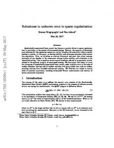
concept, and it also generated a high-accuracy digital elevation model of the Earth using synthetic aperture radar. The Gravity Recovery and Climate Experiment mission (GRACE) consists in two spacecraft flying in formation taking precise measurements of their relative states. This data allows scientists to generate the most precise gravity model of the Earth to date. This same concept was exploited by the Gravity Recovery and Interior Laboratory (GRAIL), which mapped the Moon’s gravity field. In February 2016, the LIGO team announced the detection of gravitational waves for the first time, confirming Einstein’s theory of general relativity. To extend these pioneering results the evolved Laser Interferometer Space Antenna (eLISA), consisting in three spacecraft in wide formation, will be launched in the 2030s to detect more accurately the ripples in space-time. LISA Pathfinder was launched in 2015 to test the key technologies required by eLISA, in particular the formation-keeping capabilities. When designing a telescope, the aperture of the instrument is determined by the diameter of the main mirror. This is limited by obvious practical constraints, like the diameter of the launch vehicle. For instance, the diameter of the main mirror aboard the Hubble Space Telescope is 2.4 m, just enough to fit in the space shuttle cargo bay. The James Webb Space Telescope (JWST) will replace Hubble in 2018, and the new observatory mounts a mirror of 6.5 m in diameter. The mirror cannot fit inside the Ariane 5 fairing, so the engineering team opted for a foldable mirror composed by hexagons. Although more flexible, this solution is still limited by the launcher and future concepts explore the use of multiple satellites. The Terrestrial Planet Finder concept (Fig. 1.1) involved multiple small infrared telescopes flying in precise formation, simulating an unprecedentedly large aperture observatory. In addition, having multiple collectors allows the astronomers to apply sophisticated reduction techniques in the data pipeline to subtract bright stars. Unfortunately, this mission was canceled in 2011 due to budget issues.
1.2 Distributed space systems The full potential of miniaturized spacecraft relies on operating several satellites that perform cooperative tasks, forming a distributed space system. The relative motion between small spacecraft (down to the pico-scale, weighing around 100 g) has received much attention for industrial applications in recent years. Some advanced concepts promoted by DARPA, among others, even consider the use of spacecraft swarms, with tens of thousands of spacecraft. Formation flying introduces a new paradigm of space mission design, and it is rapidly replacing monolithic solutions in many scenarios. Even the startup world is taking advantage of the wide range of possibilities provided by this concept. The San Francisco-based Planet Labs, for example, currently operates a constellation of almost a hundred 4 kg-spacecraft, which image the Earth continuously. But the potential of distributed space systems is not merely economic. It also opens a whole new world of possibilities from a scientific and operational perspective. The German TanDEMX formation flying mission (launched in 2010) served as a proof
Figure 1.1: Artistic view of the Terrestrial Planet Finder. Source: NASA.
The Kepler space telescope has discovered up to 2,327 exoplanets, improving our knowledge about extrasolar worlds and unveiling astonishing examples of bizarre planetary systems. The telescope only instrument is a photometer, which transmits lightcurves of almost 150,000 stars back to Earth. The search for exoplanets is based on the transit method: if the apparent brightness of a star decreases periodically, this could mean that a planet is orbiting it. This method has some disadvantages, like the high
§1.3 Efficient orbit transfers
3
number of false positives (around 40% for Kepler) and the fact that the only planets that can be detected are those in edge-on orbits. An interesting alternative to transit detection is the direct imaging of the planets. The telescope observes the planets themselves, instead of focusing on the central star. The challenge is that the stars are much brighter than the planets, and light reflected on them is typically lost. To solve this problem, coronographs can be placed between the telescope and the source to block the light of the star, and then the telescope is pointed to the planets. The most flexible solution is to design an occulter that flies in formation with the telescope, and blocks the light accordingly. The New Worlds mission features an occulter that will possibly fly with the JWST enabling direct observations of exoplanets. A proof of concept mission is also under development at Stanford, the Miniaturized Distributed Occulter/Telescope (mDOT). The required precision in both the relative positioning and pointing of the spacecraft make formation flying for astronomical applications one of the major challenges in future missions. Relative motion between spacecraft will soon have interplanetary applications. The InSight mission incorporates two cubesats, which will become the first to fly in deep space. Provided with both UHF and X-band antennas, the Mars Cube One (MarCO) will serve as a communication relay for InSight, specially during entry, descent and landing. The cubesats will follow their own orbits to Mars, and this poses an important challenge in regards to the navigation and operation of multiple spacecraft. Even the design team of the Europa mission, the latest of NASA’s flagship program, is considering the use of two cooperative spacecraft. After reaching Jupiter’s moon Europa along a low-energy transfer, the main spacecraft will deploy a lander that will maintain a communication link with the mothership. When the lander completes its experiments on the surface of Europa, it will take off, rendezvous, and dock to the carrier. These are just some applications showing the relevance of distributed space systems in future mission concepts.
tween the different engineering and scientific teams.
1.3 Efficient orbit transfers
In the industrial side, low-thrust electric propulsion has great potential for placing geostationary satellites into orbit. The high altitude of the geostationary orbit (GEO), which is almost 36,000 km, makes it impossible for a rocket to insert a satellite directly into this orbit. The rocket puts the spacecraft into a highly elliptical orbit with its apogee at GEO altitude, and then the satellite’s engines are used to circularize the orbit. The ABS-3A geostationary satellite (Boeing 702SP bus) was launched in March 2015 and used a revolutionary transfer strategy, as it was the first GEO satellite using electric propulsion. The spacecraft spiraled for over six months until it reached its operational orbit. Less propellant was spent in this phase and, as a result, there is more fuel available for the required station-keeping maneuvers, increasing its operational life. These corrective maneuvers compensate the drift of the satellites at GEO due to the Earth’s nonspherical gravity field. The design of a transfer using chemical propulsion consists in finding the optimal distribution of the maneuvers along the orbit, and in characterizing such maneuvers. When using electric thrusters, the engine is on for almost the entire duration of the transfer. The steering and throttling of the engine needs to be
Advances in launch systems have cut down the cost of leaving the Earth, and the use of spacecraft formations reduces the unitary cost of the craft and improves the scientific capabilities. But, once in space, the problem of reaching the final orbit still remains. A mission comes to an end when the spacecraft runs out of fuel. Thus, the propellant expenditures during the cruise phase need to be minimized, so the craft has as much fuel as possible when starting its nominal operations. Interplanetary travels are the best examples of the need for smart transfer strategies. Finding the adequate launch window is one of the key elements. For example, a 154-day transfer to Mars launched on April 18, 2018 will require a mass of propellant that is 55% of the total mass of the spacecraft. However, if the launch is delayed by only 20 days, the propellant fraction will rise to 93% to keep the same time of flight, because of the configuration of the planets. Trajectories are usually very sensitive to changes, what complicates the design process. This is particularly critical during the preliminary phases, in which there are many iterations be-
1.3.1
Low-thrust missions
The specific impulse (Isp ) of a propulsion system can be regarded as a measure of its efficiency: the higher the specific impulse, the less propellant is needed to exert the same change in the velocity of the spacecraft. Table 1.2 compares the specific impulse and maximum thrust of different propulsion systems. Solid rocket boosters deliver high-thrust levels with low specific impulses, and are good choices for launch vehicles. Once ignited, the combustion cannot be stopped. Rockets with liquid fuel (bipropellant) can be switched on and off, and they have been the preferred choice for space maneuvers. New concepts based on electric propulsion, like ion engines and the variable specific impulse magnetoplasma rocket (VASIMR), increase the specific impulse significantly, at the cost of producing smaller thrust forces. Table 1.2: Specific impulse and thrust of different propulsion systems.
Isp [s] Thrust [N]
Solid rocket
Bipropellant rocket
Ion engine
VASIMR
(STS booster)
(RS-25)
(NEXT)
(VX-50)
250
350-450
4,000
5,000
13,800,000
1,900,000
0.250
0.500
A typical space maneuver consists in switching on a chemical engine for a few minutes, which yields a change of velocity that is almost instantaneous given the total duration of the mission. But its low specific impulse makes it less efficient than electric propulsion systems. For these reason, missions like Deep Space 1, Hayabusa, or Dawn used the latter instead of the usual chemical thrusters. Given the low thrust levels of ion engines, the thruster needs to be on for months instead of minutes, and the spacecraft follows a spiral trajectory that slowly takes it to its final orbit. The mass of propellant can be reduced significantly, at the cost of increasing the time of flight.
4
1
Introduction. Current challenges in space exploration
determined, and this process turns out to be a complex optimization problem.
1.3.2 Solar sailing The Russian space pioneer Konstantin Tsiolkovsky envisioned potential alternatives to rockets like the use of solar sails that, by the effect of the solar radiation pressure, accelerate the spacecraft without spending fuel. The concept has been around for decades, but it involves some technical difficulties that have hindered its implementation in actual missions. In 2010, the Japan Aerospace Exploration Agency (JAXA) launched IKAROS, the first successful interplanetary mission provided with a solar sail. The spacecraft deployed a 200 m2 sail that propelled it to Venus. Later that year, NASA launched the NanoSail-D2 cubesat equipped with a 10 m2 solar sail. Figure 1.2 shows an artistic conception of the LightSail cubesat, launched in 2015 and promoted by the Planetary Society.
Figure 1.2: The LightSail spacecraft. Source: The Planetary Society.
The dynamics of spacecraft using solar sails are similar to the motion of probes with low-thrust electric propulsion systems. The force due to the solar radiation is small in magnitude, and it is accelerating the spacecraft continuously. This acceleration can be controlled by changing the attitude of the sail. The techniques used for low-thrust trajectory optimization can be extrapolated to the design of solar sail missions. The advantage of the latter is the fact that no propellant is required.
1.3.3
Gravity-assist trajectories
In 1966, Gary Flandro published an interesting discovery he made during a summer he spent at the Jet Propulsion Laboratory (JPL). Between 1977 and 1978, Jupiter, Saturn, Uranus, and Neptune would be aligned in such a way that a flyby at Jupiter would send a spacecraft to Saturn, a second flyby at Saturn would aim the trajectory to Uranus, and a third flyby would send the probe toward Neptune. He coined the term Planetary Grand Tour, and this sequence was exploited during the design the trajectory of Voyager 2 (see Fig. 1.3). During the close approach there is an energy exchange between the probe and the planet that is flown by. Because of the difference in their masses the change in the orbit of the planet is negligible, but the spacecraft experiences an important change in its velocity. Although Pioneer 10 was the first mission to use this technique, it showed all its potential with the Voyager program.
Figure 1.3: The orbit of Voyager 2 from 08/21/1977 (launch) to 12/01/1992, represented in the ICRF/J2000 frame.
Gravity-assist maneuvers have been widely used since the 1970s. In fact, most interplanetary trajectories involve flybys of intermediate planets in order to reduce the use of its engines. This makes the design process even more complicated for the mission analyst: determining the optimal trajectory is not about finding the most direct way, but rather to come up with the best sequence of flybys, dates, impulsive maneuvers, etc. The preliminary design becomes a counterintuitive task, with millions of possible combinations and solutions. Adequate analytical and numerical tools need to be implemented as the mission goals become more ambitious. Specially if the trajectory involves not only planetary flybys but also arcs with low-thrust electric propulsion, which need to be optimized as well.
1.4
Orbit propagation
The Pioneer 10 and 11 spacecraft were the first to visit Jupiter and Saturn, respectively, in 1973 and 1979. After reaching the two gas giants, they initiated their journey to interstellar space. But the spacecraft were not moving as they were expected to. An anomalous acceleration was reducing their speed faster than the models predicted. This phenomenon, known as the Pioneer anomaly, puzzled the scientific community for many years. In fact, it was not until 2012 when scientists agreed that the most likely cause was the effect of the emission of thermal radiation from the spacecraft. The magnitude of the anomalous acceleration was just of the order of 10−10 m/s2 , which shows how extremely accurate force models and simulations need to be. A careful analysis of Doppler data taken during the geocentric flybys of Galileo (December 8, 1990), NEAR (January 23, 1998), and Rosetta (March 4, 2005) revealed an unexpected change in their velocities, of the order of the millimeter per second. The origin of this energy gain remains a mystery, and has motivated many theories: from the existence of dark matter halos around the Earth to relativistic effects, issues with the sensors at the DSN stations, propagation errors…These anomalies are, in the end, unexpected differences between the motion predicted by the models and the actual measurements. The flyby anomaly and the Pioneer anomaly are famous ex-
§1.5 The aim of the present thesis amples, but discrepancies between the computed trajectory and the actual measurements always appear. In fact, measuring these differences can provide valuable scientific data. For example, the Juno science team, which recently completed the Jupiter orbit insertion, will study the structure of Jupiter’s interior and winds based on the deviations between the true and predicted orbits, which are obtained with numerical simulations. Numerical errors are always present, and minimizing this error is a critical task because errors in the propagation may lead to wrong scientific conclusions. From an operational point view, accurate and reliable orbit propagators are used to compute the nominal trajectory. The navigation and control teams will be in charge of making sure that the spacecraft stays on its design course. If the nominal orbit is constructed with a poor force model, adjusting maneuvers will be constantly needed, because the probe will never follow the predicted path. This is even more critical when multiple flybys are present. A close encounter has an amplifying effect on the numerical error. Therefore, the propagation must be as accurate as possible for the trajectory solution to be trusted. With examples like the Cassini mission, which has completed 120 flybys of Titan, 22 of Enceladus, and others of Iapetus, Rhea and Dione, ensuring the accuracy of the propagation becomes a complicated problem. Figure 1.4 depicts the orbit of Cassini during its first 18 months of operation, and shows the complexity of the trajectory.
Figure 1.4: The orbit of Cassini in the ICRF/J2000 frame centered at
Saturn (06/20/2004-12/01/2005).
Every effort toward more efficient and accurate propagation methods benefits almost every application in celestial mechanics. Trajectory optimization problems are interesting examples. In practice, optimization algorithms will be given a cost function to minimize. This cost function typically includes orbit propagations. Since the function will be evaluated thousands of times, the runtime needs to be as short as possible. In addition, numerical errors will make the optimizer converge to erroneous solutions, or it simply will not converge to any solution. On the other hand, the relative motion between spacecraft is sensitive to the differential effect of orbital perturbations. Numerical models are required for high-precision formation flying applications, which again involve numerical propagations.
5
1.5
The aim of the present thesis
The physics that govern the motion in space have not changed since the time Kepler formulated his celebrated laws. It is only our perception, our models, what have evolved. And depending on how a physical problem is described using a mathematical model, different conclusions may be derived. This thesis focuses on the theory of regularization, which was born in an attempt to eliminate the singularities in the equations of orbital motion. This theory can be regarded as a collection of mathematical and dynamical contrivances that provide a more adequate description of the dynamics. In the second chapter of his book The Prisoner, Marcel Proust writes: “The only true voyage of discovery, the only fountain of Eternal Youth, would be not to visit strange lands but to possess other eyes [...]” This quote captures the motivation of the dissertation. Taking regularized formulations as “new eyes”, this thesis approaches three of the main challenges in modern astrodynamics: formation flying, low-thrust mission design, and high-performance orbit propagation. The use of an unconventional formulation of the dynamics has yielded new results in these three areas, presented in the following chapters. The main application of regularization for the last 60 years, basically the age of space engineering, has been the development of improved schemes for numerical integration. By recovering the basics of the theory, this dissertation shows how regularization can be applied systematically to solve other problems of practical interest, as well as how to exploit all the advantages of these methods for conducting numerical simulations. The first part of the thesis is of theoretical nature, and focuses on regularization itself. Chapter 2 introduces the theory, justifying why it is worth seeking alternative representations of the dynamics. The different methods and techniques that lead to regularization are presented, together with their advantages. Chapter 3 is focused on a specific formulation, the KustaanheimoStiefel regularization (KS for short), and presents new results. In particular, a new theory of stability is developed resulting in a novel Lyapunov indicator for characterizing chaotic regimes. The next chapter, Chap. 4, analyzes the Dromo formulation and proposes some advances to the theory. In Chap. 5 an entirely new formulation is derived, based on the geometrical construction of Minkowski space-time. It improves the numerical integration of flyby trajectories. The last chapter of the first part, Chap. 6, describes the main software tool that has been developed along with this doctoral research. It is a propagator with high-fidelity force models and different formulations, conceived for testing their numerical performance. The second part of the dissertation includes the applications of regularization to spacecraft relative motion and low-thrust mission design. Chapter 7 presents the theory of asynchronous relative motion, a new approach to the relative dynamics in space. In Chap. 8 this same problem is solved using different formulations, each presenting particular advantages. The search for more convenient descriptions of the problem of low-thrust transfers led to the discovery of a whole new family of spiral trajectories,
6
1
Introduction. Current challenges in space exploration
called generalized logarithmic spirals. The definition and main properties of the orbits can be found in Chap. 9. In Chap. 10, the spiral Lambert problem is solved using this new family of spirals, and Chap. 11 presents a complete strategy for designing threedimensional low-thrust transfers. These results can be generalized to define other families of new orbits, with different physical interpretations ranging from solar sailing to representing the Schwarzschild geodesics (Chap. 12).
Part I
Regularization
7
“Read Euler, read Euler, he is the master of us all” —Pierre-Simon Laplace
2 Theoretical Aspects of Regularization
P
hillip Herbert Cowell (1870–1949) lived during an exciting period of dynamical astronomy, and was one of the various luminaries who contributed to the theory of the motion of the Moon. As second chief assistant at the Royal Observatory at Greenwich, he became intrigued by the discrepancies between the observed trajectory of the Moon and the predictions in Hansen’s tables. He corrected some coefficients of the periodic terms predicted by Hansen, and introduced new terms to account for long-period dynamics. With powerful perturbation theories at hand, he then focused his attention on the imminent return of Halley’s comet (it approached the Earth in 1910). Andrew C. Crommelin noticed in 1906 a difference of almost three years in the predictions of the date of the approaching return of the comet and, being Cowell’s colleague at the Greenwich Observatory, Crommelin suggested he recalculate the orbit. In 1892, 1904 and 1905 three additional moons were discovered orbiting Jupiter. Astronomers were struck by these findings, because for almost 400 years the Galilean moons were thought to be the only Jovian satellites. But on the night of February 28, 1908, an even more surprising discovery was made. A new moon was observed with a period that seemed tens of times larger than that of the Galilean moons. A direct orbit with this characteristics could not be stable according to Laplace’s classical theory, so Crommelin made a revolutionary suggestion: the orbit might be retrograde.* He then teamed up with Cowell to explore the rare motion of this object. The perturbation from the Sun attrac-
tion was so large (between six and ten percent of the attraction from Jupiter), that they did not even consider relying on the analytical theories that worked so well for the Moon. Instead, they decided to integrate the equations of motion in Cartesian coordinates by numerical quadrature. The method presented by Cowell and Crommelin (1908) was later referred to as Cowell’s method, and it is possibly the most common method for propagating orbits. It reduces to integrating the system of differential equations
* In 1975 this moon was called Pasiphae, and its orbit is indeed retrograde. Its orbital period of 764.1 days is significantly longer than the period of Io (1.8 days), Europa (3.5 days), Ganymede (7.1 days) and Callisto (16.7 days). The moon was discovered at the Royal Greenwich Observatory by astronomer Philibert J. Melotte, a colleague of Cowell and Crommelin.
Regularization is a collection of mathematical and dynamical transformations that seek a more convenient formulation of the equations of motion. In the second half of the 19th century and the first half of the 20th century regularization was mostly applied
d2 r µ + r = ap dt2 r3
(2.1)
in which r = [x, y, z]⊤ is the position vector in an inertial frame, µ is the gravitational parameter, and a p are external perturbations. Cowell himself was well aware of the power of this method and he soon applied it to the propagation of the orbit of Halley’s comet (Cowell and Crommelin, 1910). It is interesting to note that, in the mean time, Tullio Levi-Civita was looking for alternatives to the use of Cartesian coordinates in the problem of three bodies (Levi-Civita, 1903, 1904, 1920). In the N-body problem collisions may occur, meaning that the denominator in Eq. (2.1) will vanish. Thus, the equations of motion become singular and fail to reproduce the dynamics. An entire new branch of celestial mechanics was born from the pioneering studies by Levi-Civita and Peter Hansen about the three-body problem: the theory of regularization. In Sect. 2.4 we will discuss early contributions by Laplace.
9
10
2
Reviewing all the available methods and techniques for regularizing the equations of motion (or for improving its numerical behavior in general) will fill an entire book, and there will still be some missing formulations. This chapter is just devoted to presenting the foundations of regularization, together with more detailed historical notions and a review of the state of the art in the field. Section 2.1 deals with the question of whether it is worth or not to use sets of variables different from the Cartesian ones. The Sundman time transformation, one of the best known regularizing transformations, is discussed in Sect. 2.2. Sections 2.3– 2.5 present different techniques for improving the overall performance of the integration, including the stabilization of the equations of motion by embedding first integrals, or the use of orbital elements. Canonical transformations are briefly discussed in Sect. 2.6, and the concept of gauge-freedom in celestial mechanics, developed by Efroimsky and Goldreich (2003), is reviewed in Sect. 2.7.
2.1 Why bother? Cowell’s method presents a series of issues related to its numerical behavior and the form of the equations themselves. A singularity arises from the form of the potential of a particle orbiting a central mass with gravitational parameter µ = Gm, V (r) = −
µ r
Indeed, at the origin of the potential well (r → 0) the function V (r) takes infinite values. This is not only a theoretical singularity, because during close encounters and deep flybys the relative separation decreases rapidly. This singularity is even more critical in the context of the Nbody problem, where the potential takes the form V (r) = −G
∑ mi m j ||ri − r j || i< j
and becomes singular when any pair of particles (i, j) collide. Collisions in N-body simulations of stellar systems are usual, and the singularity needs to be overcome. We refer to Aarseth (2003, chap. 5) for a more detailed discussion about the need for regularization in N-body systems. The singularity also affects the velocity. The local circular velocity of a particle orbiting a central mass is simply √ µ v= r It increases as the orbit reduces its size. Thus, in the limit case when the orbit collapses to the origin (r → 0) the corresponding
orbital velocity becomes infinite. This phenomenon can also be understood in view of the conservation of the angular momentum, h = rv in a circular orbit. As the radial distance goes to zero, the velocity grows rapidly to compensate the angular momentum. Another issue related to the form of Eq. (2.1) is its behavior when integrated numerically. If one solves these differential equations in the Keplerian case (a p = 0), which is the simplest case possible, the evolution of the error is that shown in Fig. 2.1. It is computed as the difference between the solution propagated numerically and the analytic solution. Even when integrated with the Störmer-Cowell integrator and a fine tolerance (10-14 ), the error grows exponentially in time, which yields a separation of about 500 m after 20,000 revolutions. The example corresponds to a geocentric orbit with e = 0.3 and a = 8000 km. 4
10 Error [m]
in the context of the three-body problem. With the rise of computers and the Space Age in the 1960s and 1970s, the numerical integration of the equations of orbital motion received renewed interest. Regularization was no longer a mere theoretical artifact, for scientists like Joachim Baumgarte, Eduard Stiefel, or André Deprit proved that regularized schemes were better suited for numerical integration. Different formulations were published in those years with operational applications.
Theoretical Aspects of Regularization
2
10
0
10
0
5
10 Thousands of revolutions
15
20
Figure 2.1: Evolution of the propagation error of a Keplerian orbit. The orbit is integrated with a variable step-size Störmer-Cowell integrator of order nine with a tolerance of 10-14 .
The exponential growth of the error in Cowell’s method can be understood by studying the relative dynamics between two neighboring trajectories. Let r∗ define a Keplerian orbit, initially separated a distance δr0 from a reference solution r. The relative motion is governed by the equation r¨ ∗ − r¨ = −
µ ∗ µ r + 3r r r∗3
Under the assumption that the separation is small, i.e. ||δr0 || ≪ ||r0 ||, the dynamics can be linearized about the reference trajectory. Retaining only the first order terms the problem reduces to ] µ[ r¨ ∗ − r¨ ≈ − 5 r2 I − 3(r ⊗ r) ◦ δr = A(r) δr r Here I is the second-order unit tensor (represented by the identity matrix), ⊗ is the dyadic product, and ◦ denotes contraction.* This second order dynamical system can be reduced to a first order system when introducing the state vector δx that contains both the * Under this notation it is:
(a ⊗ b) ◦ c = a (b · c) The dyadic product of two rank-one tensors (vectors) results in a rank-two tensor (matrix), a1 b1 · · · a1 bn . . .. .. a ⊗ b = .. . an b1 · · · an bn It is often written in matrix form as a b⊤ , with a and b column vectors.
§2.2 The Sundman transformation relative position and velocity vectors, δr and δv: d(δx) = L(x) δx dt The linear operator L(x) is I 0 L(x) = A(x) 0 and models the linear dynamics of the system. The spectrum of the linear operator is √ √ √ µ 2µ 2µ λ1 = − 3 , λ2 = + 3 , λ3,4 = −λ5,6 = i 3 (2.2) r r r Four eigenvalues are purely imaginary and yield oscillatory modes. There are two eigenvalues with nonzero real parts, λ1 and λ2 ; the real part of λ1 is negative, whereas the real part of λ2 is positive. This yields an exponential growth of the separation, according to the law eλ2 t . The system is unstable in the sense of Lyapunov. See Bond (1982) for a connection with the stability of the numerical integration methods. The stable and unstable manifolds associated to the resulting saddle configuration relate to the right eigenvectors v1 and v2 , associated to λ1 and λ2 , respectively. If the components of the position vector in an inertial frame I are [x, y, z], the eigenvectors v1 and v2 read v1 = [−kx, −ky, −kz, x, y, z]⊤ v2 = [+kx, +ky, +kz, x, y, z]⊤ √ with k = r3/2 / 2µ. The referred instability is closely related to the choice of the independent variable. Consider two circular orbits of radii r and r + δr. Even if the relative separation is initially small, δr ≪ r, the evolution of the angular separation between the particles δϑ can be visualized thanks to a simple series expansion: √ ] √ [√ µ µ 3 µ δϑ = − t=− t δr + O(δr2 ) (2.3) 2 r5 (r + δr)3 r3 It grows secularly in time (the motion is Lyapunov unstable). However, the separation between the orbits, δr, is constant, and remains small. That is, the orbital motion is Poincaré (or orbitally/structurally) stable. Let Σ be a Poincaré section that is transversal to the flow and let p1 , p2 , . . . be the consecutive intersections of the orbit with Σ. The Poincaré map P : Σ 7→ Σ is such that pn+1 = P(pn ) and for a periodic orbit pi = p j ≡ p or Pn (p) = p. When the separation between the orbits is measured at a given time t it is defined as ||r∗ (t) − r(t)||, and grows exponentially. However, when the separation is measured at a value of the true anomaly (which is equivalent to analyzing the separation on a Poincaré section) it is ||p∗ − p||, and remains constant. This suggests that the independent variable plays a critical role when formulating orbital motion. Szebehely (1967, pp. 233–234) presents an elegant and unified treatment of the Lyapunov and structural stabilities by introducing the concepts of isochronous and normal correspondence.
11 The former yields a synchronization in physical time and therefore Lyapunov stability, whereas the latter relates to the synchronism in an angular variable and involves structural stability.
2.2
The Sundman transformation
The three-body problem is the simplest among the N-body systems, and collisions appear naturally. The Finnish astronomer Karl F. Sundman worked extensively on this problem and was well aware of the importance of regularizing the equations of motion. He introduced the time transformation* dt = r ds
(2.4)
that was later named after him. The fictitious time s replaces the physical time t as the independent variable, and behaves as an angle. For historical reasons we shall mention that LeviCivita (1906) and Bohlin (1911) also considered this transformation when regularizing the restricted three-body problem. The latter worked directly with the eccentric anomaly instead of considering it a fictitious time. The derivatives with respect to physical time transform into ( 2 ) d 1 d d2 1 d dr d = and = r − dt r ds dt2 r3 ds2 ds ds The typical notation for the derivatives with respect to fictitious time is the prime □′ , whereas dots □˙ refer to derivatives with respect to physical time. If Eq. (2.1) is rewritten in terms of the fictitious time it transforms into d2 r 1 dr dr µ − + r = r2 a p ds2 r ds ds r
(2.5)
This equation still presents problems for r → 0 although the order of the singularity has been reduced, changing the denominator from r3 to r. Additional transformations are required to achieve the complete regularization of the system. The Sundman transformation has a beneficial effect in the numerical integration process. It yields what Jörg Waldvogel calls “the slow motion movie” (Waldvogel, 2007); if the orbital motion is discretized using a fixed step in physical time, most of the points will be gathered around the apoapsis of the ellipse. Unfortunately, at periapsis, where the dynamics are faster and require a finer step size, there will be fewer points. This is shown by Kepler’s second law: given a differential dt the particle sweeps a differential of area which is constant, dA =
1 1 2 r dϑ =⇒ dϑ ∝ 2 2 r
* We refer to the memoir that the mathematician Magnus G. Mittag-Leffler invited Sundman to write on the subject in 1913 (Sundman, 1913). The results presented in that paper were a collection of previous results obtained by the author and published in different works, mainly in Recherches sur le problème des trois corps and Nouvelles recherches sur le problème des trois corps. These two papers appeared in Acta Societatis Scientiarum Fennicae, volumes 34 (1907) and 35 (1909) respectively. Although in this chapter we only recover the time transformation, we must emphasize that the most memorable result presented in Sundman’s Mémoire is the conclusion that all solutions to the regularized three-body problem can be represented by convergent series. The time transformation from Sundman (1913, eq. 71) yields a new form of the canonical system; Levi-Civita (1920, §2) referred to that transformation as the Darboux-Sundman transformation.
12
2
and dϑ is angular separation in true anomaly between consecutive points. When the particle is closer to the origin (periapsis) the angular separation grows. Conversely, when r is large (apoapsis) the points are close to each other, and yield the distribution shown in Fig. 2.2(a). On the other hand, differentiating Kepler’s equation yields dt = αr dE
(2.6)
with E the eccentric anomaly and α a constant depending on the semimajor axis and the mean motion. Identifying Eqs. (2.4) and (2.6) shows that the fictitious time s is in fact equivalent to the eccentric anomaly E, except for a constant factor affecting its time evolution. The discretization of the orbit with fixed steps in fictitious time (equivalent to E) is shown in Fig. 2.2(b).
(a) Fixed step in t
(b) Fixed step in s
= 0.8) using the physical and the fictitious times and the same number of points. Figure 2.2: Discretization of a highly elliptical orbit (e
The examples in Fig. 2.2 have been constructed with the same number of points, meaning that the integrator will take the same number of steps. However, using the discretization in physical time (Fig. 2.2(a)) yields very large steps during periapsis passage. This introduces important numerical errors because the integration fails to capture the rapid changes in the states. On the contrary, a discretization in fictitious time (Fig. 2.2(b)) leads to a finer representation of the dynamics around periapsis, and the result will be more accurate. At apoapsis, where the dynamics are much slower, the wider step size of Fig. 2.2(b) reduces the number of unnecessary steps, speeding up the integration.
2.2.1 Generalized Sundman transformation The time transformation in Eq. (2.4) is often generalized to dt = αrn ds
(2.7)
where α is an arbitrary constant and n defines the order of the transformation. Different values of n have been tested in the past century. Before diving into the possible transformations we shall first borrow a theorem from Stiefel and Scheifele (1971, p. 78): Theorem 1: (Stiefel and Scheifele, 1971, Thm. 3) Given the analytic step-size adaption in Eq. (2.7), a full regularization of the equations of motion (2.1) can only be achieved for n < 3/2. The original transformation by Sundman corresponds to n = 1 and, according to this theorem, the complete regularization of the equations of motion is possible. If the constant parameter α takes the value α = (a/µ)1/2 , the fictitious time becomes
Theoretical Aspects of Regularization
the eccentric anomaly. Many regularization methods are based on the transformation n = 1. Some examples are the formulations by Levi-Civita (1904, 1906, 1920) and later extended by Kustaanheimo and Stiefel (1965), or alternative methods by Sperling (1961), Burdet (1967), Janin (1974), Bond and Gottlieb (1989), Bond (1990), Roa and Peláez (2015d) and Baù et al. (2015), among others. The case n = 3/2 was explored by Nacozy (1977), who coined the term intermediate anomaly for referring to the fictitious time in this case. The constant factor α reads α = µ−1/2 (1 + e2 )1/2 . The intermediate anomaly relates to the true anomaly by virtue of s = ek2 F(ϑ/2, k) with k2 = 2e/(1 + e) and F(ϑ/2, k) the incomplete elliptic integral of the first kind. Nacozy’s discovery was motivated by the concept of the partial anomalies proposed by Hansen (1853), a method that he had already applied to determine the orbit of Comet Encke (Nacozy, 1969). Hansen (1853) derived a new general perturbation method for propagating cometary orbits. As the director of the Seeberg Observatory he was concerned about the accuracy of the computations. The orbits of comets are typically elliptical and cross the circular orbits of the planets. Consequently, the planetary perturbations upon the comet vary in different time scales and involve many frequencies. This phenomenon complicates the development of series solutions because they depend heavily on the natural frequencies. In order to account for the different time scales, he introduced the inferior and superior partial anomalies related to the quadrants of the ellipse. In Hansen (1853, §3, p. 57) a detailed discussion of the possible situations regarding the in-orbit position of the comet can be found. Later, Glydén (1870) improved the convergence of the series solution by introducing elliptic functions. A review of the methods can be found in a dedicated publication by Baillaud (1876). In the case n = 2 and α = 1/h, the fictitious time evolves like the true anomaly. There are a number of regularized theories based on this time transformation, for example those from Burdet (1969); Vitins (1978); Palacios and Calvo (1996); Peláez et al. (2007) and Urrutxua et al. (2015b). It is interesting to note that Burdet (1969) introduced the terms central and focal method, referring to the regularization with n = 1 and n = 2 respectively. The names come from the fact that the eccentric anomaly rotates around the center of the conic section, whereas the true anomaly is referred to the focus. Vitins (1978) and Peláez et al. (2007) exploited the gyroscopic representation of the orbital plane, the later taking advantage of the theory of ideal frames developed by Hansen (1857). We refer to Jochim (2012) for a translation of the most important parts of the original manuscript, as well as for a detailed analysis of the fundamental results. It is worth noticing that this transformation was already applied by Laplace (1799, book II, chap. 2, p. 150) when deriving his theory of orbital motion. The time transformation in Eq. (2.7) can be written in its most general form as dt = g(r) ds
(2.8)
§2.2 The Sundman transformation where g(r) , 0 is an arbitrary function. Many different forms of the function g(r) have been explored, specially for regularizing N-body systems (see Sect. 2.2.2). For example, Cid et al. (1983) addressed the dynamics of particles moving in a central force-field governed by the potential ∑ ai V (r) = ri i and introduced a time transformation with rn/2 gn (r) = √ rn−2 + b1 rn−3 + . . . + bn−2 in order to achieve the full regularization of the Hamiltonian. Ferrándiz et al. (1987) unified the transformation g3 (r) and the one proposed by Belen’kii (1981), g(r) = r3/2 (1 + br)−1/2 , by introducing the time transformation: r3/2 dt = √ ds b0 + b1 r A similar equation played a key role in the regularization and linearization (in Stiefel and Scheifele’s sense) of the radial intermediary introduced by Cid et al. (1986). The last section of the celebrated work by Kustaanheimo and Stiefel (1965) has not received much attention in the past; this section is devoted to the formal treatment of nonconservative perturbations in KS formalism. They suggested the use of a generic time transformation, in an attempt to find an adequate form of g(r) so that the angular frequency of the harmonic oscillator is preserved. In their book, Stiefel and Scheifele (1971, §19) introduced a new time variable that relates to the total energy of the particle. Thus, disturbing potentials are introduced in the time transformation improving the stability of the integration. Baumgarte and Stiefel (1974) published a dedicated analysis of other possible transformations and discussed their advantages. Satō (1998) published an ingenuous regularization of collisional orbits by representing Keplerian motion in the projective space. Thanks to this construction he arrived to the concept of the projective anomaly, a new parameterization of orbital motion that successfully regularizes the problem when r → 0. By connecting the projective anomaly with the eccentric anomaly, Satō introduced the generalized anomaly. This variable includes not only the eccentric and projective anomaly as special cases, but also the true anomaly. Kopeikin et al. (2011, §1.3.5 and §1.3.6) reviewed this concept in detail, and took advantage of its properties for exploring the gauge freedom of orbital motion (see Sect. 2.7).
2.2.2
Time transformations in N-body systems
It was Sundman (1913, §11) himself one of the first to realize that the transformation in Eq. (2.4) does not work well when there are more than two bodies. For an N-body system r is not unique, because there are N(N − 1)/2 relative distances ri j between the particles. He focused on the three-body problem and defined an alternative transformation in terms of the regularizing function ( )( )( ) g(ri j ) = 1 − e−r12 /ℓ 1 − e−r13 /ℓ 1 − e−r23 /ℓ
13 Here ℓ is a constant depending on the physical properties of the system. Finding an adequate transformation of the independent variable is a critical part of the regularizing strategy. As shown by Sundman, when there are more than two bodies it is more convenient to define a transformation involving the relative states of all the bodies. Aarseth and Zare (1974) arrived to a remarkable regularization of the three-body problem by introducing the KS transformation in order to model the dynamics of a single binary. Binary collisions are completely regularized, and the integration of triple encounters is well behaved numerically. They found a regular form of the Hamiltonian in KS variables relying on the time transformation dt = αrik r jk ds
(2.9)
Under this notation the regularized double encounters are rik → 0 and r jk → 0. Later that year, Heggie (1974) advanced on Aarseth and Zare’s method by generalizing the regularization to any pair of particles, and then extending the formulation to generic N-body systems. For that he considered the new time transformation ∏ dt = ri j ds i< j
that involves the relative separation between all the particles. In the particular case N = 3 he explored an alternative transformation r12 r13 r23 dt = ds (r12 + r13 + r23 )3/2 and found slight improvements in the accuracy and numerical performance. The special role of the exponent 3/2, which later led to the intermediate anomaly (Nacozy, 1977), will be discussed in more detail in Sect. 2.3. It is again remarkable that a transformation similar to the one in Eq. (2.9) can be found in a note by Levi-Civita.* An important breakthrough in the definition of time transformations was the introduction of conserved quantities such as the energy or the Hamiltonian in the regularizing function g. Zare and Szebehely (1975) approached the problem from a rigorous perspective looking for values of g that makes ∫ ∑ pi qi = g(2T − V ) ds i
integrable, where qi and pi are the coordinates and the momenta, and T is the kinetic energy. Noting that 2T − V = H + T = 2H + V = (3H + L)/2, with L the Lagrangian, the previous expression transforms into ∫ ∫ ∑ pi qi = g(H + T) ds = H(t − t0 )+ gT ds i
∑
∫ pi qi =
i
∑ i
∫ pi qi =
∫ g(2H + V ) ds = 2 H(t − t0 )+ g(3H + L) ds =
1 3 H(t − t0 ) + 2 2
gV ds ∫
gL ds
* Levi-Civita, T. “Sul problema piano dei tre corpi. Caso limite in cui una delle masse eè infinitesima”, Rendiconti del Lincei, 1915, 24, p. 559.
14
2
The form of the last term suggests the use of the regularizing functions g = 1/T, g∫ = 1/V or g = 1/L in order to arrive to the trivial integrals ds. Recall that the use of the potential function in the regularizing process had already been explored by Levi-Civita (1903, p. 66) and Stiefel and Scheifele (1971, §19). The transformation g = 1/L was introduced in Heggie’s method by Mikkola (1985). Thanks to this modified transformation, the referred method now allows to handle simultaneous binary collisions. In addition, the Hamiltonian adopts a more compact form that makes its differentiation with respect to canonical coordinates and momenta simpler. The resulting method is easier to implement than the original version by Heggie. The transformation g = 1/L has a remarkable implication: the fictitious time is defined by ∫ t s= L dt t0
and it is equivalent to the action integral S . Thus, the action is used as the new independent variable. The principle of least action states that δS = 0, and therefore δs = 0. The path followed by the particle is the one that minimizes the fictitious time between the departure and arrival points.
2.3 Stabilization of the equations of motion Baumgarte (1972b) proved in a seminal work that embedding conserved quantities in the system of differential equations to be integrated improves significantly the stability of the integration process. Stability in this case refers to how well the integrals of motion or dynamical constraints are conserved. This technique comes from noting that the numerical integration scheme has in general no information about the conservation laws. Thus, if they are introduced in the system they behave as control terms and reduce the error-growth rate. This technique proves useful not only in the Keplerian case, but also in presence of conservative perturbations where the total energy is conserved (Baumgarte, 1972a). Stabilization can be understood from two different perspectives, as Velez (1974) observed: the equations can be stabilized numerically and analytically. The techniques aiming for one or the other type of stabilization are similar, and reduce to: 1. Transforming the independent variable by introducing a fictitious time. 2. Linearizing the equation of motion in order to transform Eq. (2.1) into a linear oscillator. 3. Embedding the energy equation into the system of equations. An alternative to steps 2 and 3 is to integrate sets of elements instead of coordinates (Sect. 2.5 is devoted to the use of elements in orbit propagation). In the 1970s, Dr. C. E. Velez’s group did a lot of work on numerical integration of orbits at Goddard Space Flight Center, while developing the Goddard Trajectory Determination System
Theoretical Aspects of Regularization
(GTDS, see Wagner and Velez, 1972). For example, Velez (1967) presented an innovative predictor-corrector algorithm to integrate multi-revolution orbits more efficiently. Velez and Hilinski (1978) analyzed the impact of time transformations on the truncation errors when integrating Cowell’s method through a number of numerical experiments. The question about the stability of the numerical integration was further developed by Velez (1975). The system of equations (2.1) is unstable in the sense of Lyapunov. Under an adequate transformation these equations may be transformed to a harmonic oscillator, which is stable (see Sect. 2.4 for a detailed analysis of the linearization of the equations). The Lyapunov instability of the system mainly affects the propagation of the truncation error and is reduced when introducing a fictitious time. Recall the example in Eq. (2.3), which proved that the angular separation between two neighboring particles grows in time proportionally to −(3/2)r−5/2 µ1/2 . Considering now a Sundman transformation of the form dt = r ds, the separation between the particles is governed by the equation √ ] [ √ µ µ δϑ s = (r + δr) −r s (r + δr)3 r3 √ 1 µ s δr + O(δr2 ) =− 2 r3 In a normalized example (µ = 1 and r = 1) it is simply δϑ s = −(s/2) δr, whereas the separation given in Eq. (2.3) evolves as δϑt = −(3t/2) δr. The fact that δϑ s /δϑt = 1/3 is what motivated Baumgarte’s statement: the introduction of a fictitious time dt = r ds reduces the Lyapunov instability of orbital motion by a factor three (Baumgarte, 1972a). A partial analytic stabilization is achieved. Clearly, when the true anomaly is the independent variable δϑ does not change, meaning that for dt = r2 ds the system is completely stabilized in Lyapunov’s sense. Although orbital motion referred to the fictitious time is stabilized, the time transformation needs to be integrated to provide the physical time: ∫ t − t0 = g(s) ds and reducing the Lyapunov instability might not improve the numerical conditioning of this integral. The error in the propagation of the time variable is coupled with the total error of the trajectory, and it is difficult to assess its impact in the most general case. An interesting result from Velez (1974) in the case of an orbit perturbed by the J2 gravity terms of the central body is that the error growth rate is minimum for n ∼ 1.5, although the system is not strictly stabilized. The stabilizing effect of embedding first integrals in the equations of motion can be seen in the following example. Let us recover the equations of motion in terms of the fictitious time — Eq. (2.5)—, r′′ −
r′ ′ µ r + r = r2 a p r r
(2.10)
The equation of the Keplerian energy can be understood as a control term; multiplying this integral of motion by r renders [ ′ ′ ] (r · r ) µ − − Ek r = 0 r 2r2
§2.4 Linearization
15
This control term appears recursively in the literature and it is sometimes referred to as the Poincaré term (Baumgarte and Stiefel, 1974; Janin, 1974). Adding the previous two equations yields the controlled equations of motion [ ′ ′ ] r′ ′ (r · r ) ′′ r − r + − Ek r = r 2 a p (2.11) r 2r2
In presence of conservative perturbations it is possible to replace the Keplerian energy by the total energy, defining a generalized eccentric anomaly, φ. It is the variable that evolves in time like
Figure 2.3 shows the difference in accuracy between integrating Eq. (2.10) and Eq. (2.11), which includes the control term. In order to isolate the effect of the control term, the nominal orbit is considered circular. The particle orbits around the Earth and the orbital radius is 8000 km. The equations of motion are integrated using a RKF 5(4) scheme, with absolute and relative tolerances ε = 10−11 . The error growth rate of the controlled equations is smaller than the uncontrolled case. As a result, after for example 5,000 revolutions, the error in position is reduced by about three orders of magnitude, from about 500 m down to 0.5 m.
and φ(0) = E0 . The element formulations proposed by Stiefel and Scheifele (1971, §19) and Baù et al. (2015), for example, are based on this construction.
Figure 2.3: Error in position for the integration of the uncontrolled
equations (Eq. (2.10), in black) compared to the controlled equations (Eq. (2.11), in gray).
Using the energy equation as a stabilizing mechanism is particularly powerful when dealing with conservative perturbations. The perturbing acceleration derives from a disturbing potential
dφ = dt
2.4
√
−2E r
Linearization
The linearization of the equations of motion is crucial in the regularization procedure. In this context, linearization does not refer to expansions for small values of a given parameter. It means transforming a system of nonlinear equations into a system of linear equations, without neglecting any terms in the equations. The book by Stiefel and Scheifele (1971) and the essay by Deprit et al. (1994) are two of the most complete works on this particular subject. The first approach to the linear form of the equations of motion is possibly due to Laplace. We credit Deprit et al. (1994) for writing the original form of the equations by Laplace in a more friendly way.* Let C = {uρ , uθ , uz } be a rotating frame with uz normal to the reference plane, uρ defined by the projection of the position vector onto the reference plane, and uθ completing a dextral frame, uθ = uz × ur . Figure 2.4 depicts the geometry of the problem.
a p = −∇V p The total energy of the system is constant and reads E = Ek + V p Thus, the control term can be referred to the total energy, [ ′ ′ ] (r · r ) µ − − E + V p r=0 r 2r2 so the controlled system adopts the form [ ′ ′ ] (r · r ) r′ 2 r′′ − r′ + − E + V p r = r ap r 2r2 Thanks to using the total energy instead of the Keplerian energy, the constant of motion E is embedded in the system. This technique is widely applied in regularization theories. It is advantageous not only from the numerical perspective, as it might also simplify analytic formulations. In Sect. 2.2 a number of time transformations involving the potential or the energy were discussed. For instance, using the eccentric anomaly as the fictitious time, for a Keplerian orbit it is r dt = √ dE −2Ek
Figure 2.4: Geometric decomposition of Laplace's linearization.
The projected radius is ρ = r · uρ , the projected angular momentum reads λ = h · uz , and the transversal component of the motion is z = r · uz . Introducing the variables ϱ = 1/ρ, ζ = z/ρ and the transformation ds = λϱ2 dt, the equations of orbital motion * The system (K) presented by Laplace (1799, p. 151) is written in scalar form and the components of the perturbing acceleration are represented by the derivatives of a force function Q. The time transformation introducing a new independent variable is rather complicated since it involves the integral of a perturbing term.
16
2
take the form: d2 ϱ + ϱ = −ϱ (a p · uρ ) − ds2 d2 ζ + ζ = −ζ (a p · uρ ) − ds2 dλ = λ (a p · uθ ) ds
dϱ (a p · uθ ) ds dζ (a p · uθ ) + (a p · uz ) ds
2.4.1
Levi-Civita variables
Tullio Levi-Civita was particularly interested by the problem of regularizing collisions between pairs of bodies. In 1906 he suggested the introduction of a new set of coordinates for defining the planar motion, by means of his celebrated transformation in the complex plane (Levi-Civita, 1906): x + iy = (ξ + iη)2
(2.12)
which provides x = ξ2 − η2
and
y = 2ξη
and therefore x2 + y2 = (ξ2 + η2 )2
(2.13)
He achieved a global regularization of the motion when introducing a fictitious time, dt = r ds. Special attention was paid to the canonicity of the transformed system. His regularization scheme can be applied to the general perturbed two-body problem. Writing r = [x, y]⊤ and u = [ξ, η]⊤ the Levi-Civita transformation L : u 7→ r reduces to [ ] ξ −η r = L(u) u with L(u) = η ξ Matrix L(u) is the Levi-Civita matrix. Applying this transformation to Eq. (2.5) yields: 2
d u r + ω2 u = L⊤ (u) a p 2 ds2
(2.14)
It is the equation of an oscillator of frequency ω2 = −E/2, with E the energy of the system (total or Keplerian), forced by the external perturbations: dω2 = −[L(u) u′ ] · a p ds
the errors in one variable propagate rapidly to the others. In addition, Eq. (2.14) has effectively embedded the energy. Its evolution can be integrated separately in order to rake advantage of the stabilization mechanism described by Baumgarte (1972b). Figure 2.5 compares the error growth rate of Cowell’s method (already shown in Fig. 2.1) with that of Eq. (2.14). The dynamical instability has been weakened, as expected, and the final error in position is reduced by two orders of magnitude. However, the error still grows in time even for this simple case because of the instability of the time transformation. 4
10 Error [m]
The resulting differential equations are linear, and explicitly decoupled. In addition, if there are no external perturbations acting on the system (a p = 0) then the previous equations reduce to harmonic oscillators of unit frequency.
(2.15)
The derivation of Eq. (2.14) and some interesting properties of the Levi-Civita matrix can be found in Chap. 3, and also in the dedicated monograph by Stiefel and Scheifele (1971, §8). In the Keplerian case a p = 0 and Eq. (2.14) reduces to a harmonic oscillator. The differential equations are linear and decoupled, an important improvement with respect to Eq. (2.1). In the latter
Theoretical Aspects of Regularization
2
10
0
10
0
5
10 Thousands of revolutions
15
20
Figure 2.5: Evolution of the propagation error of the Keplerian orbit discussed in Fig. 2.1. The black line corresponds to the integration of Eq. (2.1), and the gray line shows the accuracy of Eq. (2.14). The latter is integrated with a variable order and variable step-size Adams scheme, setting the tolerance to 10-13 .
The volume XXIV of Rendiconti del Lincei, published in 1915, includes a total of five notes by Levi-Civita. In the first one, entitled “Sulla regolarizzazione del problema piano dei tre corpi” and presented to the Academy in July, he recovered the transformation in Eq. (2.12) and refined the regularization. The second note dives into more profound concepts related to the dynamics of a special type of holonomic system. The third (November 21) and fourth (December 5) notes focus on the canonical formalism of the three-body problem regularized by means of Eq. (2.12). Finally, his fifth note “Sul problema piano dei tre corpi. Caso limite in cui una delle masse è infinitesima” focuses on the restricted problem and explores more general forms of his transformation, namely x + iy = f (ξ + iη) He even introduced a set of elliptic coordinates thanks to the transformation x + iy = r/2 cosh(ξ + iη). Most of these results were collected in his renowned 1920 memoir. This memoir starts by reviewing the previous efforts by the author toward regularization of the three-body problem, and discusses the work done by P. Painlevé, R. Ball, and K. Sundman. It is interesting to note that Levi-Civita pointed out that Karl Weierstrass, famous for his work on elliptic functions, also contributed to the regularization of the N-body problem. Indeed, in a letter to Sophie Kowalevski* , he briefly discussed the topic and hoped to advance on it in the future. There is an intriguing phenomenon related to the transformation in Eq. (2.12): transformations of this type exist only for dimensions 1, 2, 4, and 8, as proved by Hurwitz (1898) and later * The letter dated December 16, 1874, can be found in Weierstrass’ biography by Mittag-Leffler (1912, p. 30)
§2.4 Linearization
17
by Adams (1960). Thus, is it possible to extend Levi-Civita’s regularization to three-dimensions? The answer to this problem required the joint efforts of Paul Kustaanheimo and Eduard Stiefel (Kustaanheimo and Stiefel, 1965). We save the detailed explanation of the KS transformation for Chapter 3, where the need for an extra dimension is explained. Transformations in the complex plane were also exploited by George D. Birkhoff. In 1915 he published a novel regularization of the restricted three-body problem. First, he sets the origin of the system not at the barycenter (the common practice) but at the midpoint between the primaries. By introducing the complex variable q = x + iy + 1/2 − ν (with ν the mass ratio of the primary bodies) he succeeded in reducing the problem to q¨ + 2i˙q = ∇q V (q) A concise summary of the exposition by Birkhoff (1915) was provided by Szebehely (1967, pp. 97–103). Birkhoff acknowledges that a few months before the publication of his paper Levi-Civita referred him to a previous global regularization admitting double collisions: it was the Thiele-Burrau regularization.* Other transformations like the Lemaître regularization are based on similar concepts, and were beautifully unified by Szebehely (1967, §3.8).
Let us now recover Eq. (2.5) and write it in compact form: r′′ −
(r · r′ ) ′ µ r + r = r2 a p r r2
The second term can be solved from Eq. (2.17), and when introduced in the previous expression yields ] [ ′ ′ (r · r ) µ r′′ − 2 − r = r2 a p − µe r 2r2 The terms in brackets correspond to the definition of the energy given in Eq. (2.16), meaning that r′′ − 2Er = r2 a p − µe
(2.18)
This equation needs to be integrated together with the Sundman transformation in order to compute the physical time. To achieve the stabilization described by Baumgarte (1972b) one should also integrate the evolution of the Laplace-Runge-Lenz vector, µe′ = 2(r′ · a p ) r − (r · a p ) r′ − (r′ · r) a p together with E ′ = (r′ · a p )
2.4.2 Cartesian coordinates Linearization can also be achieved relying on the usual position and velocity vectors, as Laplace’s results suggest. A major breakthrough was that of Hans Sperling and Claude Burdet, who were able to achieve the linear and regular form of the equations of motion (Sperling, 1961; Burdet, 1967). Sperling embedded the integral of motion of the energy and transformed the time variable, seeking a generalized solution to Kepler’s problem. Burdet, who was Eduard Stiefel’s doctoral student and was deeply influenced by his work in regularization, followed a similar approach but he also introduced the eccentricity vector in the formulation. We shall now derive this formulation as an illustrative example of the steps toward regularization described in Sect. 2.3: introducing a fictitious time, linearizing the nonlinear equations, and embedding integrals of motion in the formulation. First, the integrals of motion of Kepler’s problem are written in terms of the fictitious time, defined by dt = r ds. The energy takes the form v2 µ (r′ · r′ ) µ − = E= − 2 r r 2r2
(2.16)
Similarly, the Laplace-Runge-Lenz vector is defined as e=
] µ v×h r 1 [ − =⇒ µe = 2 (r′ · r′ ) r − (r′ · r) r′ − r µ r r r (2.17) * Thiele (1895) presented a transformation involving a complex transforma-
tion of the form ξ + iη = cos(E + iF), with ξ and η relating to the coordinates (x, y), and E and F defining the relative orientation of the bodies. This solution assumed that the primaries had equal masses, as it emanated from the Euler problem of three-bodies. In 1906 C. Burrau extended the method in order to account for cases different from ν = 1/2. It is remarkable that Thiele already made use of the time transformation dt = r12 r13 ds that would be adopted later by Levi-Civita.
Practical comments about the method can be found in the book by Bond and Allman (1996, §9.3). Baumgarte (1972a) and Janin (1974) followed almost the same procedure, although they did not introduce the eccentricity vector.
2.4.3
Universal solutions
Transforming the equations of orbital motion to an oscillator presents additional advantages apart from regularization and numerical stability. In absence of perturbations the angular frequency of the oscillator is defined in terms of the Keplerian energy Ek , which is constant. The sign of the frequency squared is given by the sign of the energy, or equivalently by the type of orbit (elliptic, parabolic and hyperbolic). Because Eq. (2.14) reduces to u′′ + ω2 u = 0 with ω2 = Ek /2 constant, this equation is integrated easily and the solution depends on the type of orbit: u0 cos(ωs) + (u′0 /ω) sin(ωs), Elliptic, ω2 > 0 u(s) = u0 cosh(ωs) + u′0 s, Parabolic, ω2 = 0 u0 cosh(ωs) + (u′ /ω) sinh(ωs), Hyperbolic, ω2 < 0 0 The solution can be unified by introducing the Stumpff functions Ck (z), with k their degree and z = (ωs/2)2 their argument. Namely u(s) = u0 C0 (z) + s u′0 C1 (z) A dedicated analysis of the Stumpff functions including some aspects on their implementation can be found in Appendix C .
18
2
Equation (2.18) can be solved in a similar way for the case a p = 0, resulting in r(s) = r0 C0 (4z) + s r0 C1 (4z) v0 − µs2 C2 (4z) e
(2.19)
It provides a universal vectorial solution to Kepler’s problem (see the work by Condurache and Martinuşi, 2007a, for a thorough study). In addition, the Sundman transformation dt = r ds can be integrated in closed form and yields the universal form of Kepler’s equation t − t0 = sr0 C1 (4z) + s2 r0′ C2 (4z) + µs3 C3 (4z)
t − tp =
s (6r p + s2 ) 6
(2.21)
The identity r0′ = r′0 · r0 /r0 = r0 · v0 = 0 holds because of being computed at periapsis. The time of periapsis passage is t p . The fictitious time relates to the true anomaly thanks to dϑ dϑ h h = 2 =⇒ = dt ds r r Inverting this expression and integrating from periapsis to ϑ it is ϑ s = (h/µ) tan 2 Introducing the semilatus rectum p one can write r p = p/2 and h = (pµ)1/2 , and Eq. (2.21) finally becomes √ 1 t − tp = 6
form of Lagrange’s planetary equations: da dt de dt di dt dω dt
(2.20)
This equation avoids the usual complications related to replacing the eccentric anomaly by the hyperbolic anomaly, or switching to Barker’s equation. As an exercise we shall prove that this equation indeed reduces to Barker’s equation in the parabolic case: the energy vanishes, meaning that ω = 0; provided that Ck (0) = 1/k! —see Eq. (C.1)—, and assuming that the particle departs from periapsis (r0 = r p ) it follows
( ) ϑ ϑ p3 3 tan + tan3 µ 2 2
which is, indeed, Barker’s equation (Battin, 1999, p. 150).
2.5 Sets of orbital elements Elements are the integration constants in orbital motion. Stiefel and Scheifele (1971, p. 83) extended the concept of element by stating that an element is any variable that remains constant or grows linearly with the independent variable in the Keplerian case. Under this definition the mean anomaly, for example, is considered an element. Consider the set of classical elements oe = {a, e, i, ω, Ω, M0 }, namely the semimajor axis, eccentricity, inclination, argument of periapsis, right ascension of the ascending node, and (initial) mean anomaly. Their time evolution is governed by the Gauss
Theoretical Aspects of Regularization
dΩ dt dM0 dt
] 2a2 [ re sin ϑ (˜a p · i) + p (˜a p · j) (2.22) pr ] 1[ = sin ϑ (˜a p · i) + (p + r) cos ϑ + re (˜a p · j) (2.23) p r = cos(ϑ + ω) (˜a p · k) (2.24) p 1 p+r = − cos ϑ (˜a p · i) + sin ϑ (˜a p · j) e ep r (2.25) − cot i sin(θ + ω) (˜a p · k) p r sin(ϑ + ω) = (˜a p · k) (2.26) p sin i √ ] 1 − e2 [ = (p cos ϑ − 2re)(˜a p · i) − (p + r) sin ϑ(˜a p · j) ep (2.27) =
in which p is the semilatus rectum of the orbit. The basis L = {i, j, k} is the orbital frame, defined by i = r/r, k = h/h and j = k × i. The modified perturbing term reads a˜ p = h/(n2 a3 ) a p Equations (2.22–2.27) can be integrated numerically in lieu of Eq. (2.1), obtaining the osculating classical elements at each integration step. The state vector is then solved analytically from the dynamics in a Keplerian orbit. When there are no perturbations acting on the system Eq. (2.1) reduces to d2 r µ =− 3r dt2 r
(2.28)
whereas the system of equations (2.22–2.27) abides by doe =0 dt
(2.29)
Equation (2.29) is integrated trivially and the values of the elements will not be affected by numerical errors. On the contrary, the right-hand side of Eq. (2.28) is non-zero and the solution may suffer from truncation errors. The reduction of the computational time is also a direct consequence of using Eq. (2.29) instead of Eq. (2.28). Figure 2.6 shows this phenomenon with a trivial example. A Keplerian orbit is integrated using Cowell’s method (with the Störmer-Cowell integrator of order nine) and using a set of elements. The error in the integration of the Cartesian equations of motion grows in time. Conversely, the only source of error in the propagation using elements is the numerical resolution of Kepler’s equation, and the round-off error in the transformation of the elements to the state vector. When perturbations are present the right-hand side of Eqs. (2.22–2.27) will no longer be zero. However, it scales with the magnitude of the perturbation. In practical scenarios the magnitude of the perturbations will typically be smaller than the Keplerian term. Thus, the derivatives of the elements will be small in magnitude compared to the derivatives of the coordinates. The evolution of the elements will be smoother, because they evolve with the time scale of the perturbation. All these factors are highly beneficial from a numerical perspective.
§2.5 Sets of orbital elements
19 used instead, being (Arnold et al., 2007, p. 260): Λ = L, √ ξ = + 2(L − G) cos(g + h), √ p = + 2(G − Θ) cos h,
Figure 2.6: Propagation error along a Keplerian orbit in Cartesian
coordinates (black) and using a set of elements (gray).
The classical elements have been the preferred choice for centuries due to their simplicity and intuitive interpretation.* The intrinsic singularities of the classical elements (for e = 0 and for i = 0) can be readily observed in Eqs. (2.22–2.27) and motivated researchers to propose alternative sets of elements. Broucke and Cefola (1972) suggested the use of a new set of elements, called the equinoctial elements, that avoid the referred singularities of the classical elements. In the original notation proposed by the authors they form the set {a, h, k, λ0 , p, q}, and read h = e sin(ω + Ω), k = e cos(ω + Ω), λ0 = M0 + ω + Ω, i i p = sin Ω tan , q = cos Ω tan 2 2 A slightly improved version from the implementation point of view was proposed by Walker et al. (1985). Like Euler, Lagrange, Laplace, D’Alembert, Clairaut and many other great names, Charles-Eugène Delaunay devoted himself to improving the theory of lunar motion. In the very first chapter of his book (Delaunay, 1860, pp. 1–13) he suggested the use of a new set of elements for parameterizing orbital motion, {ℓ, g, h, L, G, H} (in the original order and notation). They relate to the classical orbital elements by means of ℓ = M, √ L = µa,
g = ω, √ G = L 1 − e2 ,
h =Ω H = G cos i
Their evolution in terms of the disturbing potential is also given explicitly by Delaunay (1860, p. 13, eq. 9). The canonicity of these elements in Kepler’s problem, proved by the simplified form of the resulting Lagrange and Poisson brackets, makes them appealing for analytic studies. The interested reader is referred to works such as those by Brouwer (1959), Deprit (1981), Alfriend and Coffey (1984) or Gurfil and Lara (2014) for examples of their use. The Delaunay equations become singular for small eccentricities and inclinations, and the Poincaré elements {Λ, ξ, p, λ, η, q} are often * As a historical comment we recall that it was Johannes Kepler the one who parameterized the orbits using the eccentricity and the axes. “Ergo ellipſis eſt Planetæ iter”. With this sentence he stated that the planets follow elliptic orbits around the Sun. It is found in chapter 58 of his Astronomia Nova, published in 1609. His reasoning was based on observations of the orbit of Mars. It was not until 1775 that Leonhard Euler published his theory about the rotation of solids, entitled “Du mouvement d’un corps solide quelconque lorsq’il tourne autour d’un axe mobile” and presented in Memoires de l’academie des sciences de Berlin, vol. 16, pp. 176–227. He introduced what were later called the Euler angles. Gauss (born just two years after) already made extensive use of the angles {i, ω, Ω} in most of his work, and they also appear in the work of Laplace (1799, chap. 4).
λ=ℓ+g+h √ η = − 2(L − G) sin(g + h) √ q = − 2(G − Θ) sin h
With only 21 years, Bengt Strömgren published a special perturbation method based on a vectorial set of elements. He parameterized the orbit in terms of the instantaneous angular velocity associated to the rotation of the orbit (dΨ/dt in his original notation), the eccentricity, the mean motion, and mean longitude at epoch (Strömgren, 1929). The angular momentum vector and the Laplace-Runge-Lenz vector, constant in magnitude and direction in the Keplerian case, were exploited by Milankovitch (1939). In the work by Roy and Moran (1973) not only a more compact formulation of Milankovitch’s method was presented, but they also derived a modified method for dealing with rectilinear and quasi-rectilinear orbits. In the introduction they discussed the connection with Hansen’s lunar theory and the parameterization by Herrick (1953). The latter introduced the semimajor axis and semiminor axis vectors as the elements defining the orbit, and the mean anomaly behaved as independent variable. Recently, Rosengren and Scheeres (2014) exploited the properties of Milankovitch’s vectorial elements in Hamiltonian formalism. As an example of application they solved in closed-form the secular motion of a particle accelerated by the solar radiation pressure. Laplace noted the potential of accounting for the radial motion and the rotation of the radial direction separately (see for example the derivations leading to the system of equations labeled (H) in his “Traité de Mécanique Céleste”, p. 149). This technique was developed in all its splendor by Deprit (1975), who recovered the concept of Hansen ideal frames (see Sect. 4.1), and byFerrándiz (1988), who introduced the concept of the projective decomposition of the dynamics when developing his dimensionrising canonical transformation. Deprit’s elements and later those proposed by Vitins (1978) used quaternions for modeling the dynamics of the orbital plane. These concepts were later unified by Peláez et al. (2007), who published a new special perturbation method that they called Dromo. Chapter 4 is devoted to this particular formulation.
Time elements From a numerical point of view, the main advantage of elementbased parameterizations of orbital motion is that the propagation in the Keplerian case is trivial. Moreover, in the presence of weak perturbations the problem is still well behaved since the derivatives are small in magnitude and evolve in the time scales of the perturbations. When the physical time t is replaced by a fictitious time s the Sundman transformation needs to be integrated numerically in order to compute the physical time. In its simplest form the equation to be integrated is dt =r ds
20
2
Theoretical Aspects of Regularization
The right hand-side does not vanish (except for collision trajectories): the derivative is not necessarily small, it evolves in the time scale of orbital motion, and suffer from truncation errors even in the Keplerian case.
symmetry of the equations. In its most general form the Hamiltonian can be written
In order the time transformation to benefit from the properties of element-like variables, a time element is introduced. Stiefel and Scheifele (1971, §18) presented possibly the first dedicated analysis of the theory of time elements. They opened their presentation explaining how the mean anomaly can be considered an element, and somehow behaves as a simplified time element. They then defined a time element τ attached to the set of natural elements in KS space.
The time evolution of the Hamiltonian along a solution in phase space is governed by ( ) dH ∂H ∑ ∂H dq j ∂H dp j = + + dt ∂t ∂q j dt ∂p j dt j
Given a generic time element τ, if the perturbations vanish the evolution of the time element will reduce to dτ =γ ds where γ is constant. If γ , 0 then τ is a linear time element, whereas γ = 0 yields a constant time element. The physical time is recovered thanks to t = τ + ft (s, r, r′ ) ′
Here ft (s, r, r ) denotes a generic nonlinear function. For example, using the eccentric anomaly as the independent variable and the time of periapsis passage as the time element (τ ≡ t p ), it is 1 t = τ + (E − e sin E) n The introduction of a time element was a technique that Baumgarte (1976a) explored as part of his efforts toward stabilizing the equations of motion. Nacozy (1981) considered different definitions of the time element based on the eccentric, the true, and the intermediate anomalies. He supported his analysis with numerical examples showing the improvements in the numerical performance when propagating an orbit perturbed by the Earth’s J2 . Numerical explorations by Fukushima (2005) yielded two important conclusions about the use of time elements (in the context of the KS regularization): first, the error growth rate is reduced from quadratic to linear; second, it removes the periodic components of the error in unperturbed problems. A detailed review on time elements can be found in the work by Baù and Bombardelli (2014), where they also attached a constant and a linear time element to the set of Dromo elements.
2.6
Introducing Eqs. (2.30–2.31) in the convective term yields ) ( dH ∂H ∑ ∂H ∂H = + Qj − Pj (2.32) dt ∂t ∂q j ∂p j j This is the law of energy. If there are no canonical forces acting on the system (Q j = P j = 0) then this equation reduces to the conservation law: dH ∂H = dt ∂t This expression proves that the Hamiltonian of a conservative system is constant if it does not depend explicitly on time. Consider now a generic Sundman transformation dt = g(q, p) ds that introduces a fictitious time s. The physical time t becomes a dependent variable. We shall attach the time to the coordinates q by writing q0 = t, so the extended vector results in q = [q0 , q1 , q2 , q3 ]⊤ . In order to preserve the symmetry of the system the conjugate momentum p0 is attached to p. Following Stiefel and Scheifele (1971, chap. VIII), this construction yields the homogeneous Hamiltonian Hh = H + p0 Setting j = 0 in Eq. (2.30) leads to dq0 ∂Hh = − Q0 = 1 − Q0 dt ∂p0 The fact that q0 ≡ t shows that it must be Q0 = 0. Similarly, Eq. (2.31) renders dp0 ∂Hh ∂H ∂t ∂H =− + P0 = − + P0 = − + P0 dt ∂q0 ∂t ∂q0 ∂t
Canonical transformations
Let q = [q1 , q2 , q3 ]⊤ and p = [p1 , p2 , p3 ]⊤ be the set of generalized coordinates and momenta. Given the Hamiltonian H and the canonical forces (Q1 , Q2 , Q3 ) and (P1 , P2 , P3 ), the canonical equations of motion read dq j ∂H =+ − Qj dt ∂p j dp j ∂H =− + Pj dt ∂q j
H = H(t; q1 , q2 , q3 , p1 , p2 , p3 )
(2.30) (2.31)
with j = 1, 2, 3. The canonical force P j relates to the nonconservative perturbations and Q j is introduced to preserve the
(2.33)
If the canonical force P0 is defined as P0 = −
3 ( ∑ ∂H j=1
∂q j
Qj −
∂H Pj ∂p j
)
then Eq. (2.33) can be identified with Eq. (2.32) by making p0 ≡ −H and the canonical equation for p0 is the law of energy. In what remains of the section the canonical forces Q j and P j are neglected (Keplerian case). Using the coordinates (t, x, y, z)
§2.7 Gauge-freedom in celestial mechanics
21
and momenta (−H, x˙, y˙ , z˙), the homogeneous Hamiltonian in the Keplerian case reduces to Hh =
1 2 (p + p22 + p23 ) − √ 2 1
µ q21 + q22 + q23
+ p0
(2.34)
The canonical equations readily lead to the equations of motion and the conservation of the energy, dq0 ∂Hh =+ = 1, dt ∂p0 dp0 ∂Hh =− = 0, dt ∂q0
dq j ∂Hh =+ = pj dt ∂p j dp j ∂Hh µ =− = − 3 qj dt ∂q j r
with j = 1, 2, 3. Let G be the time transformation
G : (t; q0 , . . . , q3 , p0 , . . . , p3 ) 7→ (s; q0 , . . . , q3 , p0 , . . . , p3 ) The fictitious time s is the new independent variable, with dt = g(r) ds. The coordinates and momenta are left unchanged. Considering the transformed Hamiltonian ˜ h = g(r) Hh (q0 , . . . , q3 , p0 , . . . , p3 ) H the canonical equations take the form ˜h ∂H dq0 =+ = g(r), dσ ∂p0 ˜h ∂H dp0 =− = 0, dσ ∂q0
˜h dq j ∂H =+ = g(r)p j dσ ∂p j ˜h dp j ∂H µ =− = − 3 g(r)q j dσ ∂q j r
shows that matrix A will only be symplectic for g(r) = 1. Consequently, transformations of this type are not canonical. If A is symplectic then its inverse A
−1
= −J A ⊤ J
is symplectic too. Thus, the canonicity of a transformation can be verified both with the Jacobian of the new variables with respect to the old ones and with the Jacobian of the old variables with respect to the new ones. The condition in Eq. (2.35) can be stated in terms of the Lagrange brackets. This operator applies to any pair of variables (a, b) and is referred to a set of coordinates and momenta. It reads ) ( [ ] ∑ ∂p j ∂q j ∂p j ∂q j ∂p ∂q ∂p ∂q − = · − · a, b = ∂a ∂b ∂b ∂a ∂a ∂b ∂b ∂a j The Lagrange brackets satisfy [ ] [ ] a, b = − b, a Following the reasoning that yielded Eq. (2.35), the transformation T is canonical if it leaves the Lagrange brackets unchanged, meaning that [ ] [ ] a, b p,q = a, b p,˜ q˜ A necessary and sufficient condition for the T -invariance of the Lagrange brackets is [ ] [ ] [ ] q˜ k , q˜ ℓ = 0, p˜ k , q˜ ℓ = δi j , p˜ k , p˜ ℓ = 0 (2.36)
with j = 1, 2, 3. The transformation is a trivial canonical transformation provided that the coordinates and momenta are invariant. Since we have introduced a fictitious time, it is natural to explore the canonicity of the transformation from the physical velocity v to the fictitious velocity r′ , which leads to Eq. (2.5). There are different methods for checking the canonical nature of a generic transformation of the coordinates and momenta,
Introducing the Poisson brackets ( ) { } ∑ ∂a ∂b ∂a ∂b ∂a ∂b ∂a ∂b a, b = − = · − · ∂q ∂p ∂p ∂q ∂q ∂p ∂p ∂q j j j j j and exploiting the properties of symplectic maps the condition in Eq. (2.36) turns out to be equivalent to { } { } { } q˜ k , q˜ ℓ = 0, p˜ k , q˜ ℓ = δi j , p˜ k , p˜ ℓ = 0
˜ p) ˜ T : (q, p) 7→ (q, Denoting by A the matrix containing the partial derivatives of ˜ p) ˜ with respect to the old variables the transformed variables (q, (q, p), the transformation T is canonical if A is symplectic, i.e. ⊤
A JA
=J
with [ 0 J= −I
(2.35)
I
]
0
Taking q˜ ≡ q and p˜ = g(r)p the matrix A results in g(r)I 0 1 A= g(r) −v ⊗ ∇r g(r) I The form of the product [ ] 1 ∇r g(r) ⊗ v − v ⊗ ∇r g(r) I ⊤ A JA = −I 0 g(r)
2.7
Gauge-freedom in celestial mechanics
The elements are the constants of integration in Kepler’s problem. Considering a particular set of elements oe, the position and velocity vectors will be defined by nonlinear functions of the form r(t) = f(t; oe1 , . . . , oen )
and
v(t) = g(t; oe1 , . . . , oen )
The state vector is the solution to the unperturbed two-body problem µ d2 r =− 3r≡F 2 dt r Here F denotes the acceleration on the particle. The motion under an external perturbation ∆F is governed by the equation d2 r = F + ∆F dt2
(2.37)
22
2
The solution to the perturbed motion can be obtained through the variation of parameters technique. The method was originally developed by Euler in his works about the precession of the equinoxes (Euler, 1749) and further developed by Laplace in a series of papers entitled “Théorie des variations séculaires des élémens des Planetes”,* in which he studied the evolution of the orbital elements of the planets. In presence of perturbations the orbital elements are no longer constant, but functions of time. Thus, the solution follows from r(t) = f(t; oe1 (t), . . . , oen (t)) v(t) = g(t; oe1 (t), . . . , oen (t)) The time derivative of the position vector yields dr ∂f ∑ ∂f doei = + =g+Φ dt ∂t ∂oei d t
(2.38)
Note that it is the full derivative of the radius vector. It is defined in terms of g = ∂f/∂t and the convective terms, grouped under Φ=
∑ ∂f doe j ∂oe j d t j
(2.39)
In order for the velocity of the perturbed problem, dr/dt, to have the same form than the velocity of the unperturbed problem, g, Lagrange imposed the constraint Φ≡
∑ ∂f doe j =0 ∂oe j d t j
This ensures that the computed elements define the osculating orbit at every point. But this constraint can be relaxed in practice, as Michael Efroimsky proved in a series of works (Efroimsky, 2002, 2005). Let us transform the system (2.37) to a first order system and assume that the right-hand side is uniformly Lipschitz continuous, which is a fair assumption provided that typically the perturbing terms are continuously differentiable. The PicardLindelöf theorem readily shows that the solution (r, v) is unique. This proves that r and v are invariant to the selection of the function Φ. Different forms of Φ render different sets of nonosculating elements, but they will define the same state vector under the corresponding transformation. Motivated by this freedom of choice, Efroimsky (2002) suggested that the Lagrange constraint is rather arbitrary and it can be relaxed making Φ , 0. He referred to Φ as a gauge function, representing a reparameterization of the solution (r, v). The set of all possible definitions of the gauge function forms the gauge group, a symmetry group denoted G.
The gauge-generalized equations of motion The invariance of r(t) under the action of the symmetry group G yields relations between different sets of elements emanating * Published in Nouveaux Mémoires de l’Académie Royale des Sciences et Belles-lettres (Berlin) in three parts: the first one appeared in 1781 (pp. 199–276), the second in 1782 (pp. 169–292), and the third in 1783 (pp. 161–190).
Theoretical Aspects of Regularization
from different definitions of the gauge. In particular, denoting ˆ j , it follows the osculating elements by oe ˆ = f(t; oe) f(t; oe)
(2.40)
Similarly, the velocity matching condition renders ˆ = g(t; oe) + Φ(t; oe) g(t; oe)
(2.41)
These two systems of nonlinear algebraic equations can be solved for the nonosculating elements given the osculating ones, and vice-versa. Differentiating Eq. (2.38) once more with respect to time renders d2 r ∂g ∑ ∂g doe j dΦ + + = ∂t ∂oe j d t dt dt2 where ∂g/∂t ≡ F. Equating this result to Eq. (2.37) leads to ∑ ∂g doe j dΦ + = ∆F ∂oe j d t dt
(2.42)
If Eq. (2.39) is multiplied by ∂g/∂oen and Eq. (2.42) is multiplied by ∂f/∂oen , subtracting the resulting equations provides: ∂f dΦ ∂f ∑ ∂g doe j ∂g ∑ ∂f doe j · + · − · ∂oen d t ∂oen j ∂oe j d t ∂oen j ∂oe j d t =
∂f ∂g · ∆F − ·Φ ∂oen ∂oen
The left-hand side simplifies to ∑[ ] doe j ∂f dΦ ∂f ∂g oen , oe j + · = · ∆F − ·Φ d t ∂oe d t ∂oe ∂oe n n n j [ ] where oen , oe j are the Lagrange brackets using the position and velocity vectors as canonical variables in phase space (q ≡ f and p ≡ g), [
] ∂f ∂g ∂f ∂g oen , oe j = · − · ∂oen ∂oe j ∂oe j ∂oen
(2.43)
This result yields the gauge-generalized Lagrange planetary equations ( ) ∑[ ] doe j dΦ ∂f ∂g oen , oe j = ∆F − · − ·Φ (2.44) dt dt ∂oen ∂oen j Making Φ = 0 yields the classical form of the planetary equations. Note that this expression involves the full derivative of the gauge function, which reads dΦ ∂Φ ∑ ∂Φ doe j = + dt ∂t ∂oe j d t j Therefore, if the gauge depends on the elements Eq. (2.44) should be resorted to ) ∑ ([ ] ∂Φ ∂f doe j · oen , oe j + ∂oe j ∂oen d t j ( ) ∂Φ ∂f ∂g = ∆F − · − ·Φ (2.45) ∂t ∂oen ∂oen
§2.8 Conclusions The choice of a nontrivial gauge might have theoretical and practical advantages. Efroimsky and Goldreich (2003, 2004) showed that the gauge can be defined in order to preserve the canonicity of the formulation in presence of velocity-dependent perturbations. Gurfil and Klein (2006) found the optimal form of the gauge that minimizes the integration error of a RungeKutta scheme. Later, Gurfil (2007) exploited the gauge freedom in the problem of spacecraft relative motion in order to find new families of frozen orbits. More details can be found in the book by Kopeikin et al. (2011, §1.5.3).
2.8
Conclusions
Regularization was born from the necessity of avoiding the singularities in the three-body problem. At first, regularized theories were mathematical contrivances that helped researchers to analyze the dynamics of the system. The formulations were based on different principles, from Hamiltonian mechanics to topological transformations. During the design and operation of a space mission, however, the dynamical regime is far from the singularity and it seems that regularization is not useful. But it was soon realized that the transformations that worked so well in the three-body problem exhibited important advantages in the two-body problem too. Different techniques aim for an improved numerical scheme. For example, the introduction of special variables can potentially alleviate the negative effects that the Lyapunov instability of orbital motion has on the numerical integration of the Cartesian equations of motion. By replacing the time by an alternative independent variable one achieves an analytic step-size adaption that enhances the performance of the numerical integrator. Similarly, embedding integrals of motion in the equations behaves as a control term that slows down the error growth. The use of orbital elements to model the dynamics is advantageous in many cases. Since weakly perturbed problems are close to Keplerian orbits, in such cases the evolution of the elements will be smoother than the evolution of the coordinates. From a numerical perspective, the right-hand side of the equations to be integrated will be smaller, meaning that the problem is less sensitive to truncation errors. Recent discoveries prove that the elements need not be referred to the osculating orbit (see, for example, the work by Dosopoulou and Kalogera, 2016, which derives a physical model for mass-transferring binary systems using nonosculating elements). The freedom of choice in the dynamical modeling has great potential for analytic and numerical studies. In the following chapters the foundations of regularization are recovered and applied to different problems in astrodynamics. The techniques described in the present chapter will be exploited for finding new analytic solutions to some problems, and for deriving new formulations to describe particular phenomena.
23
R:
S0 ,→ S1 → S1
C:
S1 ,→ S3 → S2
H : S3 ,→ S7 → S4 O : S7 ,→ S15 → S8 Fibrations of hyperspheres and their correspondence to the four normed algebras: real numbers, complex numbers, quaternions, and octonions.
3
The Kustaanheimo-Stiefel space and the Hopf fibration
I
n the 1960s, Eduard Stiefel started to organize the Oberwolfach Meetings on Celestial Mechanics, in an attempt to draw the interest of mathematicians into this subject. The first of those meetings took place in 1964 and Paul Kustaanheimo presented his work on describing Keplerian motion using spinors. His work on spinors combined with Stiefel’s experience in topology and numerical calculus gave birth to the celebrated extension of the Levi-Civita transformation to the three-dimensional case, known as the Kustaanheimo-Stiefel transformation or KS for short (Kustaanheimo and Stiefel, 1965). This extension had eluded researchers since Levi-Civita (1920) presented his original regularization of the planar problem and Hurwitz (1898) and Adams (1960) proved that transformations of this type only exist in spaces of dimension n = 1, 2, 4, 8. Heinz Hopf discovered a particular transformation from the unit three-sphere S3 (a three-dimensional manifold embedded in R4 ) onto the unit two-sphere S2 (a two-dimensional manifold embedded in R3 ) so that the preimage of each point in threedimensional space turns out to be a circle on S3 , called a fiber (Hopf, 1931). All points in this fiber transform into the same point in three-dimensional space. Such transformation is referred to as the Hopf fibration. In fact, the Kustaanheimo-Stiefel transformation can be understood as a particular Hopf map (Stiefel and Scheifele, 1971, §44). Hopf was Stiefel’s doctoral advisor and influenced other areas of his research, including the Hopf-Stiefel functions and the Stiefel manifolds. Davtyan et al. (1987) developed the generalization of KS transformation to the case R8 → R5 in order to transform the problem of the five-dimensional hydrogen atom into an eight-dimensional oscillator. They successfully rewrote the Hamiltonian of the hydrogen atom as the
Hamiltonian of an eight-dimensional isotrope oscillator. Deprit et al. (1994) published an exhaustive treaty on the transformations underlying KS regularization. They focused on the topic of linearization, connecting with prior work from Lagrange. The KS transformation provides a robust regularization scheme for dealing with close approaches or even impact trajectories. Close encounters are one of the major challenges in N-body simulations. The first extensions of the KS transformation to Nbody problems are due to Peters (1968), Aarseth (1971) and Bettis and Szebehely (1971). We refer to the work of Szebehely and Bettis (1971) for a review of the methods developed in those years. Aarseth and Zare (1974) focused on the three-body problem and their method was later generalized by Heggie (1974), who reformulated the Hamiltonian for dealing with an arbitrary number of particles. The shortcoming of Heggie’s method is that it fails to reproduce collisions of more than two particles. Mikkola (1985) discovered a technique for avoiding this singularity by rewriting the Sundman time transformation in terms of the Lagrangian of the system. This method integrates 4N(N − 1) + 1 equations of motion, so its use is recommended for few-body problems. The formulations based on the KS transformation have been improved throughout the years (Mikkola and Aarseth, 1998; Mikkola and Merritt, 2008), especially since the development of the chain regularization techniques (Mikkola and Aarseth, 1989, 1993). The introduction of relativistic corrections in the models has occupied different authors: Kupi et al. (2006) modified the KS regularization for two-body close encounters in N-body simulations by introducing post-Newtonian effects; Funato et al. (1996) published a reformulation of the KS transformation focused on time-symmetric algorithms. Aarseth (1999, 2003) pre25
26
3
sented several reviews of the evolution and keystones in the development of N-body simulations. The Levi-Civita variables have recently been recovered by Lega et al. (2011) to detect resonant close encounters in the three-body problem, and used by Astakhov and Farrelly (2004) in combination with an extension of the phase space to analyze the elliptic restricted three-body problem. The topological implications and numerical performance of the KS transformation has motivated many studies on the subject. Stiefel was a committed teacher and supervised over sixty doctoral students. Some of them made significant contributions to regularization and celestial mechanics in general, names like Claude Burdet, Jiri Kriz, Gerhard Scheifele, Michael Vitins, and Jörg Waldvogel. Velte (1978) explored the representation of the KS transformation in the language of quaternions, a task that also occupied Vivarelli (1983) and Waldvogel (2006a,b). Different representations of KS regularization have been published by Vivarelli (1986, 1994), including a representation in hypercomplex algebra (Vivarelli, 1985). Hypercomplex numbers will be recovered in Chap. 5 to formulate a propagator based on the geometry of Minskowski space-time. Deprit et al. (1994) re-derived the KS transformation by doubling, using quaternions and octonions. They concluded by deriving the Burdet-Ferrándiz transformation from the foundations of KS regularization (Ferrándiz, 1988). Saha (2009) has recently reformulated the problem by combining quaternions with the Hamiltonian formalism. ElBialy (2007) approached the KS transformation from an alternative perspective, focusing on the connection with the Hopf map and the topological structure of the transformation. Moser (1970) determined the topological structure of Kepler’s problem by regularizing the energy manifold. In a series of papers, Fukushima (2003, 2004, 2005) analyzed different numerical aspects of regularization, seeking scaling factors that guarantee the conservation of the integrals of motion and time elements for improving the stability of the time transformation. Recently, Roa et al. (2016c) discovered a topological phenomenon in KS space related to the transition to chaos. By analyzing the structure supporting Hopf’s fibration they proved that numerical errors related to the exponential divergence of the orbits may break down the KS transformation, as fibers will no longer be transformed to points in three-dimensions. The first part of this chapter explains the need for an additional dimension when regularizing the three-dimensional problem. It is combined with historical notes about the relevance of this problem in mathematics. The equations of the KS transformation can be found in Sect. 3.2, with comments emphasizing the connection with the Hopf fibration. The inverse transformation is defined explicitly in terms of the Hopf map. The main contribution of this chapter is the development of a new theory of stability, by translating classical concepts to KS space (see Sect. 3.3 and Roa et al., 2016c). These new results serve as foundation for introducing the new concept of manifold of solutions and topological stability, which will lead to a novel Lyapunov indicator (Sect. 3.4). Numerical examples of N-body systems are presented in Sect. 3.5 to show the consequences of topological instabilities. Finally, in Sect. 3.6 we derive, for the first time, the gaugegeneralized equations for the elements attached to KS space, after presenting a new geometric interpretation of the elements. Sec-
The Kustaanheimo-Stiefel space and the Hopf fibration tion 3.7 serves as an appendix discussing geometrical and algebraic aspects of the KS transformation.
3.1
The need for an extra dimension: fibrations of hyperspheres
The Levi-Civita variables, introduced in Sect. 2.4.1, yield a global regularization of the planar problem. Levi-Civita himself admitted that the extension of his transformation to the threedimensional problem was not straightforward (in fact, he never achieved it): “The problem in space has long resisted my efforts, as I tried to approach it by similar coordinate changes. The usual canonical transformations relating to elliptical motion do not regularize either.” Levi-Civita (1920, p. 2, in French) Where is the difficulty coming from? Why did Kustaanheimo and Stiefel define a transformation in four dimensions? The answer comes from a classical problem in number theory, later extended to more profound topological results, related to quadratic forms of the type (x12 + . . . + xr2 )(y21 + . . . + y2s ) = z21 + . . . + z2n
(3.1)
where the terms zk are bilinear functions of xi and y j . This identity is said to be of dimension (r, s, n). It is uncertain how he arrived to this result, but in the third century Diophantus of Alexandria stated (in words) that the identity (2, 2, 2) holds for z1 = x1 y1 + x2 y2 ,
z2 = x1 y2 − x2 y1
(3.2)
The reader might observe that taking two complex numbers p = x1 − i x2 and q = y1 + i y2 this identity reduces to z = pq with z = z1 + i z2 . Under this formalism Eq. (3.1) is none other than the relation between the moduli of two complex numbers: |p|2 |q|2 = |z|2 Here |p|2 = pp† with p† the conjugate of p. Writing p = q = ξ+i η and z = x+i y one readily obtains the fundamental relation of the Levi-Civita transformation presented in Eq. (2.13), namely x2 + y2 = (ξ2 + η2 )2 Equation (3.2) becomes the Levi-Civita transformation itself, x = ξ2 − η2 and y = 2ξη. On May 4, 1748, Leonhard Euler wrote a letter to Christian Goldbach in which he noted that if p = x12 + x22 + x32 + x42 and q = y21 + y22 + y23 + y24 then pq = z21 + z22 + z23 + z24 , with z1 = x1 y1 + x2 y2 + x3 y3 + x4 y4 z2 = x1 y2 − x2 y1 − x3 y4 + x4 y3 z3 = x1 y3 + x2 y4 − x3 y1 − x4 y2 z4 = x1 y4 − x2 y3 + x3 y2 − x4 y1
§3.2 The KS transformation as a Hopf map
27
That is, he proved that Eq. (3.1) holds also for dimension (4, 4, 4). Just like the case (2, 2, 2) relates to multiplication in C, Euler’s polynomial identity is equivalent to the quaternion product (although defined almost a century before Hamilton described quaternions in 1843). Indeed, taking two quaternions p, q ∈ H defined as p = x1 − ix2 − jx3 − kx4 and q = y1 + iy2 + jy3 + ky4 , Euler’s result reduces to
circles, S1 , on the four-dimensional sphere to points on the threedimensional sphere, defining the fiber bundle S1 ,→ S3 → S2 . The KS transformation is, in fact, a particular case of the Hopf map.
z = pq
S p ,→ Sn → Sn−p
where again |p|2 |q|2 = |z|2 and z ∈ H. It took 150 years after Euler’s discovery until Adolf Hurwitz proved that this kind of construction with dimension (n, n, n) exists only for n = 1, 2, 4, 8 (Hurwitz, 1898). This is an extremely beautiful result, since these are precisely the dimensions of the four only normed algebras: real numbers, R, complex numbers, C, quaternions, H, and octonions, O.* Provided that there are no normed algebras of dimension n = 3, Kustaanheimo and Stiefel (1965) decided to move to the four-dimensional case, and then sought a transformation to three dimensions. They had the right tools since Heinz Hopf, who was Stiefel’s doctoral advisor, had already presented important results regarding the transformation of spheres from four dimensions to three dimensions (Hopf, 1931). Consider the four dimensional sphere S3 ,
which connect the spheres with (p, n) pairs (0, 1), (1, 3), (3, 7), and (7, 15). Their representation complies with R, C, H, and O, respectively.
x12 + x22 + x32 + x42 = 1 and identify R4 with C2 , i.e. (x1 , x2 , x3 , x4 ) ↔ (z1 , z2 ) = (x1 + ix2 , x3 + ix4 ). Thus, S3 admits an alternative definition: |z1 |2 + |z2 |2 = 1 Hopf introduced the mapping F : C2 7→ C × R
F(z1 , z2 ) = (2z1 z2 † , |z1 |2 − |z2 |2 ) = (y1 + iy2 , y3 )
3.2
The KS transformation as a Hopf map
Kustaanheimo and Stiefel (1965) introduced the fourdimensional vector u = [u1 , u2 , u3 , u4 ]⊤ , defined in the parametric space U4 , in order to regularize the motion in three-dimensional Euclidean space E3 . The parametric space is identified with C2 thanks to considering the pair of complex numbers (v1 , v2 ) = (u1 + iu4 , u2 − iu3 ). Introducing this pair in the Hopf fibration, Eq. (3.3) provides (y + iz, x), with: x = u21 − u22 − u23 + u24 y = 2(u1 u2 − u3 u4 ) z = 2(u1 u3 + u2 u4 )
(3.5)
By identifying (x, y, z) with the components of the position vector r in an inertial frame, Kustaanheimo and Stiefel defined the KS transformation K : U4 7→ E3 . It can be written in a compact matrix form just like the Levi-Civita transformation, x = K (u) = L(u) u
(3.3)
that is called the Hopf fibration or the Hopf map. The first component of its image is a complex number, whereas the second component is a real number. Thus, the Hopf fibration maps fourdimensional spheres to three-dimensional spheres, S3 → S2 . In addition, if we define a different point on a great circle of S3 in terms of (w1 , w2 ) = (b z1 , b z2 ) and with |b| = 1 defining the great circle, it follows
F(w1 , w2 ) = F(b z1 , b z2 ) = |b| F(z1 , z2 ) = F(z1 , z2 )
For completeness we note that a direct consequence of the fundamental theorem by Adams (1960) is that there are four admissible fiber bundles,
(3.4)
This means that every point on the great circle |b| = 1 of S3 transforms into the same point on S2 . The Hopf fibration transforms * Dickson (1919) tackled the problem described in Eq. (3.1) and referred to it as the eight square theorem. He was possibly the first to note that the resulting formulas are indeed the norm of complex numbers, quaternions, and octonions (Cayley numbers). This leads to the Cayley–Dickson construction, which generates the higher-dimensional algebras by doubling the lower-dimensional ones. They allow to define additional algebras, like sedenions with n = 16, but these are no longer normed algebras: the algebra C is commutative and associative under multiplication, H is associative but not commutative, and O is only alternative. Beyond octonions these properties are lost. Mathematicians like Ferrándiz (1988) and Deprit et al. (1994) made extensive use of these observations when deriving regularized theories. The latter connected the so called binary trees with the standard basis in hypercomplex systems related to quaternions, octonions, and sedenions.
(3.6)
simply noting that x = [x, y, z, 0]⊤ is the trivial extension to R4 of the position vector. The KS matrix L(u) reads: u1 u 2 L(u) = u3 u4
−u2 u1 u4 −u3
−u3 −u4 u1 u2
u4 −u3 u2 −u1
Alternative representations of the KS transformation have been provided by Vivarelli (1983) and Waldvogel (2006b), in the language of quaternions, spinors, and hypercomplex numbers. The properties of the KS matrix are similar to those of the Levi-Civita matrix. To emphasize the connection with Hopf’s results we refer the reader to Hopf (1931, eq. 1). He stated that the coordinates (x1 , x2 , x3 , x4 ) in R4 relate to the coordinates (ξ1 , ξ2 , ξ3 ) in R3 by means of Eq. (3.5). The KS matrix is r-orthogonal, i.e. L
−1
(u) =
1 ⊤ L (u) r
(3.7)
Every point u is KS-mapped to one single point in Cartesian space E3 . The radial distance r relates to the KS variables by means of r = u21 + u22 + u23 + u24 = ||u||2
(3.8)
28
3
The of radius √ KS 4transformation maps fibers on the three-sphere r in U to points on the two-sphere of radius r in E3 . Regularizing the equations of orbital motion by means of the KS transformation requires the time transformation due to Sundman: dt = r ds
(3.9)
which was widely discussed in the previous chapter.
3.2.1 Defining the fibers
The Kustaanheimo-Stiefel space and the Hopf fibration space that are mapped into the same point in E3 by means of the KS transformation, { } F = w(ϕ) ∈ U4 x = K (w), ∀ϕ ∈ [0, 2π) A different fiber transforms into a different point. Consequently, two fibers cannot intersect because the intersection point will then be transformed into the same point in E3 despite belonging to two different fibers (Stiefel and Scheifele, 1971, p. 271). The stereographic projection of the fibers onto E3 (see for example Griguolo et al., 2012) reveals that two fibers in KS space are connected by a Hopf link, as sketched in Fig. 3.1.
Hopf (1931) proved that the transformation from the threesphere to the two-sphere maps circles to single points, defining the structure S1 ,→ S3 → S2 . A direct consequence of the result shown in Eq. (3.4) is the fact that Eq. (3.6) is invariant under the gauge transformation R : u 7→ w, x = L(u) u = L(w) w
(3.10)
Vector w = [w1 , w2 , w3 , w4 ]⊤ takes the form: w = R(ϕ; u) = R(ϕ) u
(3.11)
where R(ϕ) is the matrix cos ϕ 0 R(ϕ) = 0 sin ϕ
0 0 − sin ϕ cos ϕ sin ϕ 0 − sin ϕ cos ϕ 0 0 0 cos ϕ
Figure 3.1: Hopf link connecting two different fibers in KS space. The Hopf fibration is visualized by means of the stereographic projection to E3 .
(3.12)
3.2.2
Let u, w ∈ U4 . The KS matrix satisfies the property
This matrix is orthogonal, and also ⊤
R
The velocity and the bilinear relation
(ϕ) = R(−ϕ)
L(u) w
= L(w) u ⇐⇒ ℓ(u, w) = 0
Being R(ϕ) orthogonal Eq. (3.11) can be inverted to provide
where ℓ(u, w) denotes the bilinear relation
u = R−1 (ϕ; w) = R(−ϕ) w
ℓ(u, w) = u1 w4 − u2 w3 + u3 w2 − u4 w1
(3.13)
The transformation R preserves the radius r, i.e.
(u · u) L(w) w − 2(u · w) L(u) w + (w · w) L(u) u = 0
r =u·u=w·w Since the radius is invariant to the selection of the point in the fiber it follows that the physical time, defined by Eq. (3.9), is R-invariant as well.* The identity in Eq. (3.10) and the rorthogonality of matrix L furnish a useful relation: w = L−1 (w) L(u) u = R(ϕ) u =⇒
In addition, if ℓ(u, w) = 0 then
⊤
L
(w) L(u) = rR(ϕ)
This property was referred to as the “reciprocity of KS-operators” by Deprit et al. (1994). It is easy to verify that ℓ(u, u) = 0 is responsible for the fourth component of L(u) u being null, and the result is the extension to U4 of a three-dimensional vector. The fourth component of L(u) w is null if, and only if, ℓ(u, w) = 0. The operator L(u) is linear, meaning that L(ku)
The angular variable ϕ parameterizes the Hopf fibration in four-dimensional space. In fact, Eq. (3.11) defines explicitly the fiber F: changing the value of ϕ defines different points in U4 that are KS transformed to the same point in E3 . This yields the definition of fiber as the subset of all points in four-dimensional * Alternative
forms of the time transformation can be found in the literature, generalized as dt/ds = g(x, x˙ ). We refer to Sect. 2.2 for a survey of transformations involving different powers of the radial distance, the potential, the Lagrangian, or combinations of the relative separations for the case of N-body problems. The vectors x and x˙ are R-invariant, so the uniqueness of the physical time is also guaranteed for more general transformations.
(3.14)
= kL(u),
L(u + w)
= L(u) + L(w)
Differentiating Eq. (3.6) with respect to fictitious time and taking into account the time transformation from Eq. (3.9) yields x˙ =
2 ′ L(u) u r
(3.15)
where x˙ = [v x , vy , vz , 0]⊤ is the velocity vector extended to R4 . Note that the fourth component is zero, which means ℓ(u, u′ ) = 0
§3.2 The KS transformation as a Hopf map
29
Moreover, Stiefel and Scheifele (1971, p. 29) proved that ℓ(u, u′ ) = 0 is a first integral of orbital motion. Provided that the KS transformation is R-invariant, it follows that the bilinear relation holds for all points in a given fiber, ℓ(w, w′ ) = ℓ(u, u′ ) = 0
(3.16)
Let t(ϕ) ∈ U4 denote the vector that is tangent to a fiber F at w(ϕ). The direction of t can be obtained by differentiating Eq. (3.11) with respect to ϕ. It reads t = R∗ (ϕ) u
Introducing this expression in Eq. (3.18) and pre-multiplying the result by L−1 (u) yields u′′ +
] 1 [µ r − (u′ · u′ ) u = L⊤ (u) a p r 2 2
The term in brackets turns out to be equivalent to the Keplerian energy of the system, Ek : ] 1 ( µ v2 ) 1 [µ Ek ′ ′ ω = − (u · u ) = − =− r 2 2 r 2 2 2
In sum, the perturbed two-body problem reduces to
where R∗ (ϕ) = dR(ϕ)/dϕ is obtained by differentiating Eq. (3.12). Taking as an example ϕ = 0 yields the components of the tangent vector t,
u′′ + ω2 u =
t = [−u4 , u3 , −u2 , u1 ]⊤
under the KS regularization
(3.17)
This unveils a geometric interpretation of the bilinear relation ℓ(u, v) = 0: it can be understood as an orthogonality condition (Stiefel and Scheifele, 1971, §43), since ℓ(u, v) = 0 ⇐⇒ v · t = 0 Two vectors u and v satisfy the bilinear relation ℓ(u, v) = 0 if v is orthogonal to the fiber through u. Provided that ℓ(u, u′ ) = 0 holds naturally and it is an integral of motion it follows that the velocity in KS space, u′ , is always orthogonal to the fiber at u. The fiber bundle S1 ,→ S3 → S2 shows that the fibers constituting the three-sphere are circles, corresponding to points on the twosphere. Indeed, the tangent vector t(ϕ) is always perpendicular to the position vector w(ϕ), { [ ] [ ] [ ]} w · t = R(ϕ) u · R∗ (ϕ) u = u · R⊤ (ϕ) R∗ (ϕ)u = 0
3.2.4
(u · u) ⊤ L (u) a p 2
(3.19)
The inverse mapping
The inverse KS transformation K −1 : x 7→ u maps points to fibers. Let us introduce the auxiliary vector v = [v1 , v2 , v3 , v4 ]⊤ , defined by the mapping v1 = R sin θ 1 v2 = (y sin θ − z cos θ) 2R 1 (y cos θ + z sin θ) v3 = 2R v4 = −R cos θ
(3.20)
no matter the value of ϕ. Section 3.7 is devoted to the definition of orthogonal bases and a cross product in U4 .
Here R2 = (r + |x|)/2. The angle θ is different from ϕ: the points on the fiber are parameterized by θ, which is measured with respect to a certain axis; given two points u and w obtained by setting θ = θ1 and θ2 in Eq. (3.20), respectively, they relate by virtue of Eq. (3.11). This equation then provides the relation:
3.2.3 The two-body problem
θ2 − θ1 = ϕ
Equation (2.5) governs the evolution of the two-body problem in terms of the fictitious time s. Using the notation introduced in the present chapter it takes the form x′′ −
r′ ′ µ x + x = r2 a p r r
The point u is finally defined as
Vector a p denotes the perturbing acceleration, with a null fourth component in order to extend it to four dimensions. Differentiating Eq. (3.10) with respect to fictitious time renders ( µ ) r3 rL(u′ ) u′ + L(u) ru′′ − r′ u′ + u = a p 2 2 The fictitious radial velocity r′ transforms into r′ =
r · r′ = 2(u · u′ ) r
Identifying w ≡ u′ , Eq. (3.14) provides the relation [ ] rL(u′ ) u′ = L(u) 2(u · u′ ) u′ − (u′ · u′ ) u
meaning that the variable ϕ denotes the angular separation between points along the same fiber. The value of θ depends on the position of the reference axis, whereas ϕ is independent from the selection of the origin of angles.
(3.18)
u = [v1 , v2 , v3 , v4 ]⊤ u = [v2 , v1 , v4 , v3 ]⊤
if x ≥ 0 if x < 0
(3.21)
Two alternative expressions are considered for avoiding potential singularities. They differ in the selection of the axes in KS space. From this result any point w0 in the initial fiber F0 can be obtained attending to w0 (ϕ) = R(ϕ) u0 w0 (ϕ) = R(−ϕ) u0
if x0 ≥ 0 if x0 < 0
(3.22)
so that x0 = L(w0 )w0 . The sign criterion complies with the different definitions of axes in KS space. See Sect. 3.7 for a discussion about the orthogonal frames attached to the fiber. The linear
30
3
form of the inverse transformation has been defined by Roa and Peláez (2015f) and can be found in Sect. D.3. The velocity in U4 is obtained by inverting Eq. (3.15), taking into account the orthogonality relation in Eq. (3.7): u′ =
1 ⊤ ˙ L (u) x 2
The Kustaanheimo-Stiefel space and the Hopf fibration formulate a fundamental property of the KS transformation: Theorem 2: (Roa et al., 2016c) The angular separation between two trajectories emanating from F0 , measured along every fiber, is constant. That is w0 = R(ϕ0 ) u0 =⇒ w(s) = R(ϕ0 ) u(s)
The geometry of the inverse KS transformation can be studied from Fig. 3.2. The gray sphere is three-dimensional and of radius r. The black arc corresponds to a set of initial conditions r j on the sphere. The white dot represents one particular position in E3 , ri . The inverse KS transformation applied to ri yields the fiber Fi . The fiber is represented by means of its stereographic projection to R3 . The black surface consists of all the fibers F j that are KS mapped to the points r j . In this figure it is possible to observe the Hopf link connecting different fibers.
for any value of ϕ0 and the fictitious time s. This is an intrinsic property of KS space and does not depend on the dynamics of the system. Proof: Consider two trajectories in KS space, u = u(s) and w = w(s), departing from the same fiber F0 . They relate by means of Eq. (3.11). In the most general case the angle ϕ can be described by a function ϕ = ϕ(s) and initially it is ϕ(0) = ϕ0 . The trajectories evolve according to w(s) = R(ϕ; u(s)) = R(ϕ)u(s)
(3.23)
Differentiating this equation with respect to fictitious time yields w′ (s) = R′ (ϕ) u(s) + R(ϕ) u′ (s)
(3.24)
Equation (3.16) proved that the bilinear relation holds for any trajectory in KS space, meaning that ℓ(w, w′ ) = ℓ(u, u′ ) = 0. This renders: ) ( ℓ(w, w′ ) = ℓ R(ϕ)u, R′ (ϕ) u + R(ϕ) u′ = 0 Figure 3.2: Stereographic projection to E of the Hopf fibration 3
corresponding to a set of initial positions on the three-dimensional sphere of radius r. The black semi-torus consists of all the fibers that transform into the semi-circumference on the two-sphere on the bottom-left corner. One single fiber Fi is plotted in white, corresponding to ri .
after substituting Eqs. (3.23) and (3.24). Expanding the bilinear relation in the previous expression shows that ) ( dϕ ℓ R(ϕ)u, R′ (ϕ) u + R(ϕ) u′ = r + ℓ(u, u′ ) = 0 ds
(3.25)
Assuming that r > 0 and considering that ℓ(u, u′ ) = 0 one gets dϕ = 0 =⇒ ϕ(s) = ϕ0 ds
3.3 Stability in KS space The classical concepts of stability from Lyapunov and Poincaré can be translated to KS language by considering the topology of the transformation. First, we introduce an important new theorem regarding the geometry of the fibers (Roa et al., 2016c). From this theorem the concept of the fundamental manifold arises naturally. The stability concepts presented here are not based on numerical analyses; previous studies about the stability of KS transformation (Baumgarte, 1972a, 1976b; Arakida and Fukushima, 2000) focused on the behavior of the numerical procedure. We aim for a series of definitions that capture the physical behavior, which should be independent from the formulation of the dynamics.
3.3.1
A central theorem
Two fibers can never intersect, as discussed when formally defining a fiber. It is now possible to advance on this statement and to
so the angular separation along every fiber remains constant. We emphasize that no assumptions about the dynamics have been made. ■ A direct consequence of this result is the relation between the velocities along the trajectories u(s) and w(s): w′ (s) = R(ϕ; u′ (s))
3.3.2
The fundamental manifold Γ
A trajectory in Cartesian space, understood as a continuum of points in E3 , is represented by a continuum of fibers in U4 . Each fiber is KS transformed to a point of the trajectory. The fibers form the fundamental manifold, Γ, as Roa et al. (2016c) suggested. Equation (3.22) defines the initial fiber F0 , which yields a whole family of solutions parameterized by the angular variable ϕ. Every trajectory w(s) is confined to the fundamental manifold. Thanks to Thm. 2 the manifold Γ can be constructed following a
§3.3 Stability in KS space
31
3.3.4
Relative dynamics and synchronism
The theories about the local stability of dynamical systems are based on the relative dynamics between nearby trajectories. The concepts of stability formalize how the separation between two (initially close) trajectories evolves in time. But the concept of time evolution requires a further discussion because of having introduced an alternative time variable via the Sundman transformation. Figure 3.3: Construction of the fundamental manifold. The mapping
gt : x0 7→ x(t) denotes the integration of the trajectory from t0 to t. Similarly, g s refers to the propagation using the fictitious time.
simple procedure: first, a reference trajectory u(s) is propagated from any point in F0 ; then, mapping the transformation R over it renders a fiber Fi for each point u(si ) of the trajectory. The set ∪i Fi defines Γ. Recall that ∩ Fi = ∅ i
The fact that all trajectories emanating from F0 are confined to Γ is what makes an arbitrary choice of θ in Eq. (3.20) possible. The diagram in Fig. 3.3 depicts the construction of the fundamental manifold Γ.
3.3.3 Fixed points, limit cycles and attractors Points in E3 transform into fibers in U4 . Thus, a fixed point in Cartesian space, x0 , translates into a fixed fiber in KS space, F0 . Asymptotically stable fixed fibers (to be defined formally in the next section) attract the fundamental manifold of solutions, Γ → F0 . Asymptotic instability is equivalent to the previous case under a time reversal. Limit cycles are transformed to fundamental manifolds, referred to as limit fundamental manifolds Γ0 . A fundamental manifold Γ originating in the basin of attraction of a limit fundamental manifold will converge to it after sufficient time. For Γ → Γ0 convergence means that each fiber in Γ approaches the corresponding fiber in Γ0 . Correspondence between fibers is governed by the t-synchronism.* In a more general sense, attractors in U4 are invariant sets of the flow. The point-to-fiber correspondence connects attractors in E3 with attractors in KS space. The basin of attraction of an attractive set Yu ⊂ U4 is built from its definition in three dimensions. Let X ⊂ E3 be the basin of attraction of Y. It can be transformed to KS space, X → Xu , thanks to (
Xu = ( R ◦ K −1 )(X) = R K −1 (X)
)
This construction transforms arbitrary sets in E3 to U4 . The inverse KS transformation constitutes a dimension raising mapping, so in general dim(Xu ) = dim(X) + 1. * A dedicated discussion about the synchronism of the solutions can be found in Chapter 7. An interesting and closely related concept is the isochronous correspondence defined by Szebehely (1967, p. 233).
Keplerian motion is known to be Lyapunov unstable (see Chap. 2 for details). Small differences in the semimajor axes of two orbits result in a separation that grows in time because of having different periods. However, Kepler’s problem transforms into a harmonic oscillator by means of the KS transformation, with the fictitious time being equivalent to the eccentric anomaly. The resulting system is stable: for fixed values of the eccentric anomaly the separation between points in each orbit will be small, because of the structural (or Poincaré) stability of the motion. These considerations are critical for the numerical integration of the equations of motion. But in this chapter we seek a theory of stability in U4 expressed in the language of the physical time t, because of its physical and practical interest. The conclusions about the stability of the system will be equivalent to those obtained in Cartesian space. The spectrum of the linearized and normalized form of Kepler’s problem written in Cartesian coordinates, d2 r r =− 3 2 dt r exhibits one eigenvalue with positive real part, λ = (2/r3 )1/2 — see Eq. (2.2)—. Lyapunov’s theory of linear stability states that the system is unstable. Under the action of the KS transformation Kepler’s problem transforms into d2 u h =− u 2 ds2
(3.26)
where h is minus the Keplerian energy. Although the linear analysis is not useful in this case, selecting a candidate Lyapunov function V(u, u′ ) = h(u·u)/4+(u′ ·u′ )/2 the stability of the system is proved. In order to represent the Lyapunov instability of the motion with respect to time t the Sundman transformation needs to be considered. Given two circular orbits of radii r1 and r2 , the time delay between both solutions reads ∆t = t2 − t1 = (r2 − r1 )s The time delay grows with fictitious time and small values of r2 − r1 do not guarantee that ∆t remains small. This phenomenon relates to the synchronism of the solutions (Roa et al., 2015a; Roa and Peláez, 2016c). Solutions to the system defined in Eq. (3.26) are stable if they are synchronized in fictitious time, but unstable if they are synchronized in physical time. We adopt this latter form of synchronism for physical coherence.
32
3
The Kustaanheimo-Stiefel space and the Hopf fibration
3.3.5 Stability of the fundamental manifold
Σ, the Poincaré map P renders
Lyapunov stability
P(pn ) = pn+1
A trajectory r(t) in E3 is said to be Lyapunov stable if, for every small ε > 0, there is a value δ > 0 such that for any other solution r∗ (t) satisfying ||r(t0 ) − r∗ (t0 )|| < δ it is ||r(t) − r∗ (t)|| < ε, with t > t0 . In KS language trajectory translates into fundamental manifold. In order to extend the definition of Lyapunov stability accordingly, an adequate metric d to measure the distance between manifolds is required.
The generalization of the Poincaré section to KS space K : Σ → Σu results in a subspace embedded in U4 . In Sect. 3.2.2 we showed that the trajectories intersect the fibers at right angles, provided that the velocity u′ is orthogonal to the vector tangent to the fiber. Thus, every fiber defines a section that is transversal to the flow. The transversality condition for Σ translates into the section containing the fiber at u. The Poincaré section Σu can be constructed by combining the set of fibers that are KS transformed to points in Σ. Let n = [n x , ny , nz ]⊤ be the unit vector normal to Σ in E3 , projected onto an inertial frame. The Poincaré section takes the form
Let Γ1 and Γ2 be two (distinct) fundamental manifolds. The fibers in Γ1 can never intersect the fibers in Γ2 . But both manifolds may share certain fibers, corresponding to the points of intersection between the two resulting trajectories in Cartesian space. The distance between the manifolds at t ≡ t(s1 ) = t(s2 ) is the distance between the corresponding fibers. Setting θ to a reference value θref in Eq. (3.20) so that θ1 = θ2 ≡ θref , we introduce the metric: ∫ 2π 1 d(t; Γ1 , Γ2 ) = ||w1 (s1 ; ϕ) − w2 (s2 ; ϕ)|| dϕ (3.27) 2π 0 with d(t; Γ1 , Γ2 ) ≡ d(F1 , F2 ). It is measured by computing the distance between points in Γ1 and Γ2 with the same value of ϕ, and then integrating over the entire fiber. It is defined for given values of physical time, and not fictitious time. The reason is that the goal of this section is to define a theory of stability such that the fundamental manifold inherits the stability properties of the trajectory in Cartesian space. This theory is based on the physics of the system, not affected by a reformulation of the equations of motion. Consider a fundamental manifold Γ, referred to a nominal trajectory r(t), and a second manifold Γ∗ corresponding to a perturbed trajectory r∗ (t). If the nominal trajectory is Lyapunov stable, then for every εu > 0 there is a number δu > 0 such that d(t0 ; Γ, Γ∗ ) < δu =⇒ d(t; Γ, Γ∗ ) < εu If the initial separation between the manifolds is small it will remain small according to the metric defined in Eq. (3.27). The nominal solution r(t) is said to be asymptotically stable if ||r(t)−r∗ (t)|| → 0 for t → ∞. Similarly, the fundamental manifold Γ will be asymptotically stable if d(t; Γ, Γ∗ ) → 0 for sufficiently large times. The opposite behavior d(t; Γ, Γ∗ ) → ∞ corresponds to an asymptotically unstable fundamental manifold. It behaves as if it were asymptotically stable if the time is reversed. Poincaré maps and orbital stability The notion of Poincaré (or orbital) stability is particularly relevant when analyzing the fundamental manifold due to its geometric implications. Kepler’s problem is unstable in the sense of Lyapunov but it is orbitally stable: disregarding the time evolution of the particles within their respective orbits, the separation between the orbits remains constant. The definition of the Poincaré map in E3 involves a twodimensional section Σ that is transversal to the flow. Denoting by p1 , p2 ,… the successive intersections of a periodic orbit with
Σ ≡ n x (x − x0 ) + ny (y − y0 ) + nz (z − z0 ) = 0
(3.28)
where (x0 , y0 , z0 ) are the coordinates of the first intersection point. Equation (3.28) can be written in parametric form as Σ(x(η, ξ), y(η, ξ), z(η, ξ)), with η and ξ two free parameters. The extended Poincaré section Σu is obtained by transforming points on Σ to KS space and then mapping the fibration R: Σu = ( R ◦ K −1 )(Σ) The choice of the Poincaré section Σ is not unique, and therefore the construction of Σu is not unique either. The resulting Poincaré section Σu is a subspace of dimension three embedded in U4 . Indeed, the transformation ( R ◦ K −1 )(Σ) provides: Σ 7→ Σu (u1 (η, ξ, ϕ), u2 (η, ξ, ϕ), u3 (η, ξ, ϕ), u4 (η, ξ, ϕ)) meaning that points in Σu are fixed by three parameters, (η, ξ, ϕ). The dimension is raised by ( R ◦ K −1 ). The intersection between a given fundamental manifold and the Poincaré section Σu results in a fiber, Γ ∩ Σu = F Successive intersections can be denoted F1 , F2 ,…The Poincaré map in U4 , P : Σu → Σu , is
P(Fn ) = Fn+1 Every point in a fiber intersects Σu simultaneously. Due to the R-invariance of the Sundman transformation the time period between crossings is the same for every trajectory connecting Fn and Fn+1 . Let Γ denote a fundamental manifold representing a nominal periodic orbit, and let Γ∗ be a perturbed solution. They differ in the conditions at the first Σ-crossing, F1 and F1∗ respectively. The manifold Γ is said to be Poincaré (or orbitally) stable if d(F1∗ , F1 ) < δu =⇒ d(Pn (F1∗ ), F1 ) < εu If the separation between the fibers at the first crossing is small, the separation will remain small after n crossings.
§3.4 Order and chaos
3.4 Order and chaos In the previous section we generalized the key concepts of dynamical stability to KS space. The approach we followed aims for a theory that captures the physical properties of the system, instead of focusing on its purely numerical conditioning. The next step is the analysis of chaos in U4 . Chaotic systems are extremely sensitive to numerical errors due to the strong divergence of the integral flow. This is specially important in the vicinity of singularities, and it is precisely here where KS regularization exhibits all its potential. This section focuses on characterizing the exponential divergence of trajectories in U4 due to highly unstable dynamics. By definition the fundamental manifold is mapped to a trajectory in E3 . The equations of motion in U4 are no more than a reformulation of a dynamical system originally written in E3 . For sufficiently smooth perturbations the Picard-Lindelöf theorem ensures the uniqueness of the solution. Thus, the corresponding fundamental manifold is also unique and its KS transform defines only one trajectory. This means that any trajectory in the fundamental manifold is mapped to the same exact trajectory in E3 , no matter the position within the initial fiber. An observer in three-dimensional space, unaware of the extra degree of freedom introduced by the gauge R, will always perceive the same trajectory no matter the values of ϕ.
3.4.1
The K -separation
In order to integrate the equations of motion numerically in U4 the initial values of u0 and u′0 need to be fixed. This means choosing a point in the fiber F0 . Since all the points in F0 are KS transformed to the same exact state vector in E3 , the selection of the point is typically arbitrary. But for an observer in U4 different values of ϕ yield different initial conditions, and therefore the initial value problem to be integrated may behave differently. Ideally* all trajectories emanating from F0 remain in the same fundamental manifold, that is unique. However, numerical errors leading to the exponential divergence of the trajectories can cause the trajectories to depart from the fundamental manifold. In other words, after sufficient time two trajectories originating from the same fiber F0 , w0 = R(ϕ; u0 ), will no longer define the same fiber F(s), w(s) , R(ϕ; u(s)). In this case Thm. 2 will be violated. Multiple fundamental manifolds will appear, obtained by mapping the transformation R over each of the trajectories. The observer in E3 will see a collection of trajectories that depart from the same exact state vector and they separate in time, as if the problem had a random component. This behavior can only be understood in four dimensions. These topological phenomena yield a natural way of measuring the error growth in KS space without the need of a precise * Due
to the limited precision of floating-point arithmetic, even the fact that all points generated with Eq. (3.22) and varying ϕ will be KS-transformed to the same exact point in E3 should be questioned. The loss of accuracy in the computation of the initial conditions in U4 will eventually introduce errors of random nature. As a result, Eq. (3.22) provides points that are not exactly in the true fiber. Although the separation is small (of the order of the round-off error) and negligible in most applications, it may have an impact on the numerical integration of chaotic systems.
33 solution. Let u(s) be a reference trajectory in U4 , and let w(s) be a second trajectory defined by w0 = R(ϕ; u0 ). It is possible to build the fundamental manifold Γ from the solution u(s). The second solution is expected to be w∗ (s) = R(ϕ; u(s)) by virtue of Thm. 2. When numerical errors are present w(s) and its expected value w∗ (s) (the projection of the fundamental manifold) may not coincide. Note that w(s) = w∗ (s) ensures the uniqueness of the solution, but says nothing about its accuracy. The separation between w(s) and its projection on Γ is an indicator of the breakdown of the topological structure supporting the KS transformation, meaning that the solutions can no longer be trusted. Motivated by this discussion we introduce the concept of the K -separation, dK dK (s) = ||w(s) − w∗ (s)|| = ||w(s) − R(ϕ; u∗ (s))||
(3.29)
defined as the Euclidean distance between an integrated trajectory and its projection on the manifold of solutions. Monitoring the growth of the K -separation is a way of quantifying the error growth of the integration. In the context of N-body simulations, Quinlan and Tremaine (1992) discussed how the separation between nearby trajectories evolves: the divergence is exponential in the linear regime when the separation is small, but the growth rate is reduced when the separation is large. At this point the separation might be comparable to the interparticle distance. The K -separation will grow exponentially at first (for dK ≪ 1) until it is no longer small (dK ∼ O(1)), and then its growth slows down. Locating the transition point is equivalent to finding the time scale tcr in which the solution in KS space can no longer be trusted: for t < tcr the topological structure of U4 is preserved, but for t > tcr the uniqueness of the manifold of solutions Γ is not guaranteed. For t < tcr the R-invariance of the Sundman transformation holds. The time for all the points in a fiber coincides. Thus, tcr and scr are interchangeable: at t < tcr it is also s < scr . The behavior of the solutions can be equally analyzed in terms of the physical or the fictitious time. In practice the K -separation is evaluated as follows: 1. Choosing a reference θ in Eqs. (3.20) and (3.21), for example θ = 0, integrate u∗ (s). 2. Propagate a second trajectory w(s) generated from Eq. (3.22) with ϕ , 0. 3. Build the expected trajectory w∗ (s) by mapping R(ϕ) over u∗ (s), i.e. w∗ = R(ϕ)u∗ .The K -separation is the Euclidean distance between w(s) and w∗ (s).
3.4.2
Topological stability
The uniqueness of Γ can be understood as topological stability. KS space is said to be topologically stable if all the trajectories emanating from the same fiber define a unique manifold of solutions, and therefore they are all KS-transformed to the same trajectory in E3 . For an observer in E3 a topologically unstable system seems non-deterministic, with solutions departing from the same initial conditions but separating in time with no apparent reason.
34
3
A system is topologically stable in the interval t < tcr . The trajectories diverge exponentially, dK (t)/dK (0) ∼ eγt t
or
dK (s)/dK (0) ∼ eγs s
Here γ is equivalent to a Lyapunov exponent. For t > tcr this equation no longer models the growth of the K -separation and the system is topologically unstable. Simulations over the transition time tcr integrated in U4 can no longer be trusted. Depending on the integrator, the integration tolerance, the floating-point arithmetic, the compiler, etc. the values of tcr for a given problem might change. Thus, topological stability is a property of a certain propagation, which requires all the previous factors to be defined. The validity of the solution for an integration over the critical time tcr is not guaranteed. When tcr < tesc (with tesc denoting the escape time) not even the value of tesc can be estimated accurately. In such a case solutions initialized at different points in the fiber may yield different escape times. The method presented in this section provides an estimate of the interval in which the propagation is topologically stable. The exponent γ depends on the integration scheme and the dynamics, but it is not strongly affected by the integration tolerance. An estimate of the value of γ provides an estimate of the critical time for a given integration tolerance ε. Assuming dK (tcr ) ∼ 1: tcr ∼ −
1 log ε γt
The Kustaanheimo-Stiefel space and the Hopf fibration Heggie-Mikkola’s method is implemented in Fortran. The Hamiltonian nature of the N-body problem has motivated the use of symplectic integrators. These algorithms do not suffer from the long-term accumulation of the error in the conservation of the energy (Wisdom and Holman, 1991; Sanz-Serna, 1992). Symplectic integrators rely on a fixed-step integration, which hinders the integration of close encounters. Although Duncan et al. (1998) developed SYMBA, a multi-step and truly symplectic integrator that adjusts the step size according to the perturbations, and Chambers (1999) invented a hybrid symplectic integrator that deals with close encounters using a conventional integrator, conventional integrators with variable step size are preferred for numerical explorations of binary encounters because handling the integration step size is critical (Mikkola, 1983; Hut and Bahcall, 1983; Bacon et al., 1996; Mikkola and Tanikawa, 1999). As Mikkola recommends, we will integrate the problem with the Bulirsch and Stoer (1966) extrapolation scheme (Hairer et al., 1991, §II.9). See also the work by Murison (1989) for an analysis of the performance of this integrator in the three-body problem. The total K -separation is computed by combining the K -separations for the relative dynamics of each pair of bodies. Writing ui j ≡ uℓ it is √∑ 2 dK dK = ,ℓ ℓ
(3.30)
Conversely, if the simulation needs to be carried out up to a given t f , the required integration tolerance is approximately ε ∼ e−γt t f This simple criterion proves useful for tuning and evaluating the numerical integration. In the following examples of application the values of γt are estimated by finding the slope of the exponential growth of the K -separation in logarithmic scale. Although more rigorous algorithms could be developed, this approximation provides a good estimate of transition time between regimes.
3.5 Topological stability in N -body problems Two examples of N-body problems are analyzed in this section. The first example is the Pythagorean three-body problem. The second example is a non-planar configuration of the four-body problem. This problem simulates the dynamics of two field stars interacting with a stellar binary. The experiments are designed for showing the practical aspects of the new concept of stability introduced in this chapter: the topological stability of KS space. The problems are integrated using the regularization of the N-body problem based on the KS transformation proposed by Mikkola (1985) as a reformulation of the method by Heggie (1974). The initialization of the method is modified so that different points on the initial fiber F0 can be chosen. This means generalizing the relative coordinates ui j to wi j by means of the transformation R : u 7→ w. The trajectories depart from the same initial conditions in E3 . We inherit the normalization proposed in the referred paper, so that the gravitational constant is equal to one.
where dK ,ℓ is the K -separation computed for uℓ . Murison (1989) for
3.5.1
The Pythagorean three-body problem
Originally developed by Burrau (1913), the Pythagorean problem consists in three particles of masses m1 = 3, m2 = 4, and m3 = 5. The particles will be denoted (1), (2), and (3). At t = 0 the bodies are at rest and lying on the vertices of a Pythagorean right triangle of sides 3, 4, and 5. The initial conditions are summarized in Table 3.1. This problem has been solved and discussed in detail by Szebehely and Peters (1967), so the solution to the problem is known. Table 3.1: Initial configuration of the Pythagorean problem. ``Id'' refers to the identification index of each body. Id
x
y
z
vx
vy
vz
(1)
1.0000
3.0000
0.0000
0.0000
0.0000
0.0000
(2)
-2.0000
-1.0000
0.0000
0.0000
0.0000
0.0000
(3)
1.0000
-1.0000
0.0000
0.0000
0.0000
0.0000
The solution is displayed in Fig. 3.4. Initially the bodies approach the origin and after a number of close-approaches body (1) is ejected along a trajectory in the first quadrant, whereas (2) and (3) form a binary that escapes in the opposite direction. The escape occurs at approximately tesc ∼ 60. The solution shown in the figure is obtained by setting the integration tolerance to ε = 10−13 . The problem is first integrated from a set of initial conditions obtained with θ = 0 in Eq. (3.20). Then, a second trajectory
§3.5 Topological stability in N -body problems
35 Table 3.2: Dimensionless initial conditions for the binary system, (1,2), and the field stars, (3) and (4). ``Id'' refers to the identification index of each star. Id
Figure 3.4: Solution to the Pythagorean three-body problem. The
thick dots represent the initial configuration of the system.
x
y
z
vx
vy
vz -0.0100
(1)
0.6245
0.6207
0.0000
-0.7873
0.0200
(2)
0.6245
-0.6207
0.0000
0.7873
0.0200
0.0100
(3)
3.0000
3.0000
3.0000
-0.3000
-0.3000
-0.3000
(4)
-5.0817
-3.0000
-3.0000
0.3000
0.2333
0.3000
The manifold of solutions is constructed from a reference solution with θ = 90 deg. A second solution with θ = 120 deg (or ϕ = 30 deg) is propagated and the corresponding K -separation is plotted in Fig. 3.6. The are two different regimes in the growth of the K -separation: the first part corresponds to the linear regime where the K -separation is small, whereas in the second part the separation is no longer small. Both regimes are separated by tcr ∼ 42, when solutions in E3 no longer coincide. This result is in good agreement with the value predicted by Eq. (3.30), which is tcr ∼ 40. Since for t = tcr the bodies have not yet escaped and the integration continues, the solution is topologically unstable. The escape time associated to the reference solution, tesc ∼ 75, might not be representative because it corresponds to the interval t > tcr .
Figure 3.5: K -separation for the Pythagorean problem computed
from a reference trajectory with θ
= 0 and ϕ = 120 deg.
initialized with θ ≡ ϕ = 120 deg is integrated and their K separation is shown in Fig. 3.5. After a transient the separation grows exponentially with γt ∼ 5/12, and no transitions are observed until the escape time (tcr > tesc ). As discussed in the previous section this is equivalent to saying that the K -separation remains small, and consequently the integration in U4 is topologically stable. The transformed solution in E3 will be unique no matter the initial position in the fiber F0 .
3.5.2 Field stars interacting with a stellar binary This second example analyzes the gravitational interaction of a binary system (1,2), of masses m1 = m2 = 5, with two incoming field stars (3) and (4) of masses m3 = m4 = 3. The initial conditions, presented in Table 3.2, have been selected so that both field stars reach the binary simultaneously.
Figure 3.6: K -separation for the four-body problem computed from a reference trajectory with θ = 90 deg and a second trajectory with ϕ = 30 deg.
A direct consequence of the topological instability of the integration is the fact that solutions departing from the initial fiber F0 no longer represent the same solution in E3 . Figure 3.7 shows two solutions that emanate from different points of the initial fiber. Ideally they should coincide exactly; but because the integration is topologically unstable for t > tcr the difference between both solutions becomes appreciable and the accuracy of the integration over tcr cannot be guaranteed. The topological instability is not directly related to the conservation of the energy. Although for t > tcr the integration becomes topologically unstable, Fig. 3.8 shows that the energy is conserved down to the integration tolerance until tesc , well beyond tcr . This is a good example of the fact that the preservation of the integrals of motion is a necessary but not sufficient condition for concluding that a certain integration is correct. The evolution of the K -separation depends on the integra-
36
3
The Kustaanheimo-Stiefel space and the Hopf fibration
Figure 3.9: K -separation for the four-body problem for different integration tolerances. The solutions for ε = 10-15 and 10-17 are computed in quadruple precision floating-point arithmetic.
Figure 3.7: Two solutions to the four-body problem departing from
the same fiber F0 : the top figure corresponds to θ = 90 deg, and the bottom figure has been generated with θ = 120 deg.
where V is a disturbing potential and p refers to the perturbations not deriving from any potential. With this, Eq. (3.19) transforms into [ ] d2 u V r ∂V 2 ⊤ +ω u=− u− − 2L (u) p (3.31) 2 4 ∂u ds2 under the KS transformation. The angular frequency ω relates to the total energy E by means of ( ) E 1 µ v2 1 2 ω =− = − − V = − (Ek + V ) 2 2 r 2 2 It differs from the Keplerian energy Ek by the disturbing potential V . The relation in Eq. (3.14) combined with Eq. (3.15) renders a useful expression: L(u
Figure 3.8: Relative change in the energy referred to its initial value,
(E(t) − E0 )/E0 .
′
) u′ =
between the velocity and the derivative of u.
3.6.1 tion scheme and the tolerance. In order to analyze this dependency Fig. 3.9 shows the results of integrating the problem with four different tolerances and of changing from double to quadruple precision floating-point arithmetic. It is observed that refining the integration tolerance might extend the interval of topological stability. However, the dynamics of the system remain chaotic and the solutions will eventually diverge for sufficiently long times.
3.6 Gauge-generalized elements in KS space Stiefel and Scheifele (1971, §19) attached a set of vectorial elements to KS space, with important advantages from the numerical integration perspective. In this section we provide a new outlook into the geometry of the elements and present, for the first time, the gauge-generalized elements in KS space. The perturbation can be decomposed in a p = −∇V + p
(x · x˙ ) v2 x˙ − x 2 4
Natural sets of elements: geometric interpretation
Differentiating Kepler’s equation in the unperturbed case yields the time evolution of the eccentric anomaly. The result can be inverted to provide an alternative form of Sundman’s transformation: r dt = dE 2ωk
(3.32)
where ωk is the natural frequency referred to the Keplerian energy, ωk = (−Ek /2)−1/2 . The eccentric anomaly replaces the fictitious time as the independent variable, E = 2ωk s. Derivatives with respect to E, denoted by □∗ , relate to the derivatives with respect to s by means of 1 d d = dE 2ωk ds The velocity, given in Eq. (3.15), transforms into x˙ =
4ωk ∗ L(u) u r
(3.33)
§3.6 Gauge-generalized elements in KS space
37
Introducing the eccentric anomaly as the new independent variable and neglecting the perturbations the right-hand side of Eq. (3.31) vanishes, and the solution is simply u(E) = u0 cos
E E + 2u∗0 sin 2 2
(3.34)
The initial conditions u0 = u(0) and u∗0 = u∗ (0) are defined in terms of the position and velocity at E = 0. The state at periapsis, written in the perifocal frame P = {iP , jP , kP }, reads r0 = r p iP
and
v0 =
√
µ(1 + e)/r p jP
ˆ in U4 . Figure 3.10: Elliptic orbit in the L-plane spanned by (ˆ a, b)
with r p the radius at periapsis. The radius at apoapsis will be denoted ra . Let aˆ , bˆ ∈ U4 be the representation of vectors iP and jP in √ KS space. The initial conditions r0 and v0 yield u0 = r p aˆ and √ ˆ These expressions transform Eq. (3.34) into u∗0 = ra /4 b. u(E) =
E √ E √ r p aˆ cos + ra bˆ sin 2 2
(3.35)
By KS-transforming the expression defining u0 it follows x0 = L(u0 ) u0 = r p L(ˆa) aˆ =⇒ iP = L(ˆa) aˆ We have relaxed the notation by not distinguishing the unit vector iP from its extension to U4 , because the fourth component vanishes. Similarly, vector u∗0 transforms into √
] µ(1 + e) [ L(ˆ a) bˆ =⇒ jP = L(ˆa) bˆ rp
This equation and its derivative can be inverted to provide
4ωk ∗ x˙ 0 = L(u0 ) u0 = rp
E E) 1 ( aˆ = √ u cos − 2u∗ sin rp 2 2 ( ) 1 E E bˆ = √ u sin + 2u∗ cos 2 2 ra
ˆ = 0 holds, it is L(ˆa) bˆ = Provided that the bilinear relation ℓ(ˆa, b) ˆ ˆ ˆ . Note that vector b can be written bˆ = 2ra−1/2 u∗0 , and L(b) a therefore ˆ bˆ L(b)
The vectors aˆ and bˆ satisfy the bilinear relation √ ˆ = a 1 − e2 ℓ(u0 , u∗0 ) = 0 ℓ(ˆa, b) 2 Equation (3.35) shows that the motion in the parametric space ˆ This plane U4 is confined to the plane spanned by vectors aˆ , b. is in fact a plane of Levi-Civita’s type,* or an L-plane, provided ˆ = 0 holds. The L-plane attached to aˆ that the relation ℓ(ˆa, b) and bˆ is the representation of the orbital plane in U4 . Vector aˆ determines the direction of the major axis, and bˆ corresponds to the minor axis. Figure 3.10 depicts the geometry of the problem in the parametric space U4 . Equation (3.35) is in fact the equation of an ellipse centered at the origin. It is worthy emphasizing that vector u is not referred to the focus of the ellipse, but to its center. The minor and major axes correspond to the square roots of the radii at periapsis and apoapsis, respectively. The position in the ellipse is given by the half angle E/2. The ellipse is contained in the Lˆ plane defined by the vector elements (ˆa, b). * Stiefel and Scheifele (1971, §43) defined an L-plane as the twodimensional plane in U4 passing through the origin and spanned by two vecˆ = 0. This definition can tors aˆ , bˆ ∈ U4 satisfying the bilinear relation ℓ(ˆa, b) be extended to state that any pair of vectors in the L-plane satisfy the bilinear relation. The transformation to planes in the Cartesian space is a Levi-Civita mapping, which doubles the angles and squares the distances.
=
4 x0 ∗ ∗ L(u ) u = − ra 0 0 rp
This result yields a useful relation ˆ bˆ L(b)
= −L(ˆa) aˆ
ˆ It is Finally, it is worth proving the orthogonality of aˆ and b. † shown by the inner product aˆ · bˆ = [L⊤ (ˆa) iP ] · [L⊤ (ˆa) jP ] = iP · [L(ˆa) L⊤ (ˆa) jP ] = iP · j P = 0 ˆ Since aˆ and bˆ are unit vectors the linear operators L(ˆa) and L(b) are orthogonal —see Eq. (3.7)—. Equipping the KS space with a cross product as defined in Sect. 3.7.2 one can prove that kP = ˆ SelectiP × jP is given by the first three components of aˆ × b. ing, for example the definition from Eq. (3.58) given by Vivarelli ˆ aˆ × b} ˆ are mutually orthog(1987), the vectors in the triple {ˆa, b, onal. Consider now the more general problem in which p , 0 and V , 0. The eccentric anomaly E is replaced by a generalized eccentric anomaly, φ. The new independent variable is given a dynamical definition: it evolves with an angular velocity of the † Recall the general property of the inner product involving vectors x, y ∈ Rn and a matrix A ∈ Rn×n :
(A x) · y = x · (A⊤ y)
38
3
same form than the time rate of change of the Keplerian eccentric anomaly —Eq. (3.32)—: dt r = dφ 2ω
We seek a solution of the form
At departure the generalized eccentric anomaly coincides with the eccentric anomaly. Both angles in the parametric space U4 relate by means of (3.38)
The angle σ/2 is the angle traversed by the osculating perifocal ˆ due to the perturbations. If no perframe, defined by aˆ and b, turbations are considered (V = 0 and p = 0) the generalized eccentric anomaly coincides with the eccentric anomaly. Their evolution relates by the expression dσ dφ dE = − dt dt dt where dE/dt is the full derivative of the osculating eccentric anomaly. It can be obtained by differentiating Kepler’s equation with respect to time, taking into account the convective terms from the rate of change of the elements. The generalized eccentric anomaly is measured from a particular reference frame. This frame, referred to as the intermediate frame A, is the one that rotates with respect to the perifocal frame P with angular velocity ωA/P
1 dσ ˆ = (ˆa × b) 2 dt
The intermediate frame is defined dynamically. At departure it coincides with the perifocal frame, so that iA has the direction ˆ define the perifocal frame in U4 , that differs of e0 . Vectors (ˆa, b) from the intermediate frame in a rotation of magnitude σ/2. In what remains of the chapter the generalized eccentric anomaly is used as the independent variable. For the sake of simplicity we shall use the symbol □∗ for derivatives with respect to φ. Taking the generalized eccentric anomaly as the new independent variable the equations of motion become d2 u u + =Q dφ2 4
(3.39)
Here Q defines the forcing terms: { [ ]} 1 ∂V 1 dω du ⊤ Q=− 2V u + r − 2L (u) p − ∂u ω dφ dφ 16ω2
u(φ) = a(φ) cos
(3.40)
φ φ + b(φ) sin 2 2
(3.41)
where vectors a, b ∈ U4 are elements of the unperturbed motion. Introducing Eq. (3.38) and equating to Eq. (3.35) yields the linear ˆ and (a, b): transformation between the elements (ˆa, b) σ √ ˆ σ − ra b sin 2 2 σ √ ˆ σ √ b = r p aˆ sin + ra b cos 2 2 a=
√
r p aˆ cos
Recall that in the unperturbed problem it is σ = 0. Thus, a and b will be equal to aˆ and bˆ multiplied by the square root of the radius at periapsis and apoapsis, respectively. The determinant of the resulting (linear) transformation is √ a 1 − e2 . This result shows that the transformation is not a rotation, in general. Only when the orbit is circular vectors (a, b) ˆ by a rotation of amplitude σ/2 and will be obtained from (ˆa,√ b) a dilation of magnitude a. This can also be understood geometrically; let γa denote the angle between a and aˆ , and γb the angle between b and aˆ . They can be solved from the previous equations: √ tan γa = −
1+e σ tan , 1−e 2
√ and
tan γb = +
1+e σ cot 1−e 2
to prove that γa , −σ/2 and γb , −(π + σ)/2 except for e = 0. In general, vectors a and b will not be orthogonal. The inner product a·b=
r p − ra sin σ 2
shows that only if σ = 0 or r p = ra the vectors (a, b) will form a set of orthogonal elements. The former occurs when no perturbations are considered. The latter requires the eccentricity to be null during the entire motion. This will only occur under very specific conditions, for example an initially circular orbit subject only to perturbations that are normal to the orbital plane. The norm of a and b reduces to ||a|| = a +
The evolution of the natural frequency ω is governed by the differential equation: dω r ∂V 1 ∗ ⊤ =− 2 − [u · L (u)p] dφ 2ω 8ω ∂ t
The first term vanishes when the disturbing potential does not depend explicitly on time.
(3.36)
The Keplerian natural frequency ωk is replaced by the frequency related to the total energy E √ √ −E µ − rV ω= = (3.37) 2 2(r + 4 ||u∗ ||2 )
φ= E+σ
The Kustaanheimo-Stiefel space and the Hopf fibration
r p − ra sin σ 2
and
||b|| = a −
r p − ra cos σ 2
showing that they are not unit vectors, in general. The geometry of the orbital problem in U4 is sketched in Fig. 3.11. The origin of the generalized eccentric anomaly is the intermediate frame A. When mapped to the parametric space U4 frames P and A relate by a rotation of magnitude σ/2. The osculating eccentric anomaly is measured with respect to the perifocal frame.
§3.6 Gauge-generalized elements in KS space
39 The symmetry of these equations yields a simple form of the Lagrange and Poisson brackets. The only nonzero terms are [ ] [ ] ai , bi = − bi , ai = 1/2 } { } { ai , bi = − bi , ai = 2 in which ai and bi are the components of a and b, and i = 1, 2, 3, 4. Following the procedure presented in Sect. 2.7 we define the gauge as Φ=
∂f da ∂f db da φ db φ ◦ + ◦ = cos + sin ∂a dφ ∂b dφ dφ 2 dφ 2
(3.45)
Its full derivative takes the form
Figure 3.11: Geometrical interpretation of the elements a and b in
the L-plane.
The state of the particle in U4 has been parameterized in terms of the vector elements a and b. The total energy or, more precisely, the natural frequency ω, is the ninth element. When no perturbations act on the system these variables are constant and their numerical integration is trivial. Note, however, that the time transformation (3.36) needs to be integrated even in the pure Keplerian problem. For the sake of improving the numerical performance of the method the physical time is decomposed in (Stiefel and Scheifele, 1971, p. 92) t =τ−
1 (u · u∗ ) ω
(3.42)
where τ is a time element, governed by the perturbations. Differentiating this expression yields the equation of evolution of the time element: { [ ]} dτ 1 r ∂V ⊤ = (µ − 2rV ) − u· − 2L (u) p dφ ω3 ∂u 16ω3 2 dω − 3 (u · u∗ ) (3.43) ω dφ When the disturbing terms vanish the time element grows linearly in time. Incorporating the time element the problem is completely defined by a set of ten orbital elements, oe j (with j = 1, . . . , 10). They are the natural frequency ω, the time element τ, and the components of the four-vectors a and b.
3.6.2
Gauge freedom in KS space
In the following lines we extend the concept of the gauge freedom to the natural elements in KS space. As discussed in the previous section in absence of perturbations Eq. (3.39) reduces to a harmonic oscillator that admits the trivial solution φ φ u(φ) = a cos + b sin ≡ f(φ; a, b) (3.44) 2 2 with a and b constant. In addition, the velocity in U takes the form
dΦ ∂Φ ∂Φ da ∂Φ db = + ◦ + ◦ dφ ∂φ ∂a dφ ∂b dφ Equation (2.44) translates to KS language as ( ) ∑[ ] doe j dΦ ∂f ∂g =− Q+ · − ·Φ oen , oe j dφ dφ ∂oen ∂oen j with
{ [ ]} 1 ∂V 1 dω du ⊤ Q= 2V u + r − 2L (u) p + 2 ∂u ω dφ dφ 16ω It renders the gauge-generalized form of Eq. (19,52) from Stiefel and Scheifele (1971, p. 89): ( ) da dΦ φ φ (3.47) = +2 Q + sin + Φ cos dφ dφ 2 2 ( ) db dΦ φ φ = −2 Q + cos + Φ sin (3.48) dφ dφ 2 2 Equation (3.40) defined the evolution of the osculating total energy. Because of the gauge invariance of this variable this equation still holds and defines the evolution of the energy as: dω r ∂V 1 ∗ ⊤ =− 2 − [u · L (u)p] dφ 2ω 8ω ∂ t
(3.49)
The decomposition of the time in a secular part and a time element is G-independent so Eq. (3.43) still holds. Equations (3.50–3.51) include the full derivative of the gauge. But this term involves the derivatives of the elements, as shown by Eq. (3.46). It is then convenient to rearrange these equations so that the derivatives of the corresponding elements are all grouped in the left-hand side: ( ) ( ) ∂Φ φ φ ∂Φ da = +2 Q + sin + I cos + 2 Φ (3.50) M(φ) dφ ∂φ 2 2 ∂b ( ) ( ) db ∂Φ φ φ ∂Φ M(φ) = −2 Q + cos + I sin − 2 Φ (3.51) dφ ∂φ 2 2 ∂a This is achieved by introducing the matrix
4
φ b φ a u∗ (φ) = − sin + cos ≡ g(φ; a, b) 2 2 2 2
(3.46)
M(φ)
=I−2
∂Φ φ ∂Φ φ sin + 2 cos ∂a 2 ∂b 2
with I the identity matrix of dimension four.
40
3
In sum, the gauge-generalized equations of motion in KS space are: { [ ]} r ∂V dτ 1 ⊤ (µ − 2rV ) − u· = − 2L (u) p dφ ω3 ∂u 16ω3 2 dω − 3 (u · u∗ ) (3.52) ω dφ dω r ∂V 1 ∗ ⊤ =− 2 − [u · L (u)p] (3.53) dφ 2ω 8ω ∂ t [ ( ) ( ) ] da ∂Φ φ φ ∂Φ = M−1 +2 Q + sin + I cos + 2 Φ dφ ∂φ 2 2 ∂b (3.54) [ ( ) ( ) ] ∂Φ φ φ ∂Φ db = M−1 −2 Q + cos + I sin − 2 Φ dφ ∂φ 2 2 ∂a (3.55) The equations are completed with the initial conditions: √ µ − r0 V0 φ0 = E0 : τ = 0, ω = , a = a0 , b = b0 2(r0 + ||u′0 ||2 ) The non-osculating elements a0 and b0 are solved from the osculating elements a˜ 0 and b˜ 0 given the equations f(φ0 ; a˜ 0 , b˜ 0 ) = f(φ0 ; a0 , b0 ) g(φ0 ; a˜ 0 , b˜ 0 ) = g(φ0 ; a0 , b0 ) + Φ(φ0 ; a0 , b0 )
(3.56) (3.57)
Recall that f = a cos(φ/2) + b sin(φ/2) and g = ∂f/∂φ. The choice of the gauge must make the matrix M(φ) regular.
3.7 Orthogonal bases 3.7.1 Basis attached to the fiber In Section 3.2.2 it is shown that fibers are circles in U4 . Let u and w = R(ϕ; u) be two vectors attached to a fiber F. They span a plane containing the fiber. This plane is not a plane of the Levi-Civita type because ℓ(u, w) , 0. Since trajectories intersect fibers at right angles this subspace is transversal to the flow. An orthogonal basis can be attached to the resulting plane, allowing projections on the transversal subspace. Although arbitrary orthonormal bases can be constructed via the Gram-Schmidt procedure (Nayfeh and Balachandran, 2004, pp. 529–530), the basis described in this section appears naturally in the formulation. Associated to every vector u there is a KS matrix L(u). The columns of the matrix define a vector basis B = {u1 , u2 , u3 , u4 }, with u1 ≡ u. The basis B is orthogonal, u · u = rδi j i
j
Here δi j denotes Kronecker’s delta. Assuming x ≥ 0 every point in the fiber generated by w = R(ϕ; u) lies in the plane spanned by u1 and u4 , i.e. w · u2 = w · u3 = 0 for all ϕ. Conversely, for x < 0 the fiber is confined to the u2 u3 plane. The basis B is an orthogonal basis attached to the fiber at u. In addition, u4 · u′ = ℓ(u, u′ ) = 0
The Kustaanheimo-Stiefel space and the Hopf fibration meaning that u′ is perpendicular to u4 . In fact, u4 = −t, as shown by Eq. (3.17). The vectors arising from the products L(u)ui , i = 1, 2, 3 have a vanishing fourth component. They are equivalent to vectors in E3 . However, the fourth component of the product L(u)u4 is not zero. The three vectors obtained by these transformations correspond to the position vector r, and a pair of orthogonal vectors spanning the plane tangential to the two-sphere at r in E3 . These vectors are the columns of the associated Cailey matrix.
3.7.2
Cross product
Stiefel and Scheifele (1971, pp. 277–281) sought a definition of cross product in the parametric space U4 when discussing the orthogonality conditions of vectors and Levi-Civita planes. Although the cross product of two vectors in R3 is intuitive, its generalization to higher dimensions is not straightforward. Independent proofs from different authors (see for example Brown and Gray, 1967) show that the cross product of two vectors only exists in dimensions 1, 3, 7; for n dimensions the cross product involves n − 1 vectors. Stiefel and Scheifele (1971) defined the product p = u × v as p = L(u) v4 where v4 = [v4 , −v3 , v2 , −v1 ]⊤ is the fourth column of L(v). The properties of this construction motivated the authors to call (p1 , p2 , p3 ) the cross product of u × v, with p4 = u · v. In the following lines we analyze in more detail this construction and connect with alternative definitions provided by Vivarelli (1987) and Deprit et al. (1994). Let {e1 , e2 , . . . , en } be an orthogonal basis in Rn . The Grassmann exterior product gives rise to the bivectors ei ∧e j , trivectors ei ∧ e j ∧ ek , and successive blades of grade m ≤ n (Flanders, 1989, ∧ §II). They constitute the subspaces m Rn of the exterior algebra: ∧
Rn = R ⊕ Rn ⊕
2 ∧
Rn ⊕ . . . ⊕
n ∧
Rn
∧ ∧ noting that 0 Rn = R and 1 Rn = Rn . Without being exhaustive we simply recall that such exterior algebra is associative with unity, satisfying ei ∧ e j = −e j ∧ ei and ei ∧ ei = 0. The exterior product of two parallel vectors vanishes. We shall write ei j...k = ei ∧ e j ∧ . . . ∧ ek for brevity. In Section 3.7.1 an orthogonal basis attached to u was defined, where two of its vectors are KS-transformed to vectors spanning E3 . Identifying √ the plane tangent to the two-sphere in 1 2 3 4 i u = r ei , the exterior product of vectors {u , u , u , u } generates the oriented hypervolume u1 ∧ u2 ∧ u3 ∧ u4 = −r2 e1234 provided that det(L(u)) = −r2 . In three dimensions the exterior product is equivalent to the cross product, given e1 × e2 = e3 , e1 × e3 = −e2 and e2 × e3 = e1 . Applying the cross product to the first three elements of B provides u1 × u2 × u3 = ru4 This result confirms that B is, indeed, an orthogonal basis.
§3.8 Conclusions
41
Vivarelli (1987) and Deprit et al. (1994) worked in the more general Clifford algebra Cl3 . Introducing the Clifford product of two vectors ab = a · b + a ∧ b the exterior algebra over R3 can be identified with the Clifford algebra Cl3 : bivectors and trivectors become ei ∧ e j → ei e j and e1 ∧ e2 ∧ e3 → e1 e2 e3 . Note that ba = a · b − a ∧ b , ab, so the Clifford product is not commutative. Thus, the even subalgebra ∧ Cl+3 = R ⊕ 2 R3 , isomorphic to the quaternion algebra H, is not commutative either. The algebra H ≃ Cl+3 is endowed with the multiplication rules e21 = e22 = e23 = −1, and the product of vectors is anticommutative, ei e j = −e j ei . Identifying these bivectors with the quaternion basis elements e2 e3 = i,
e3 e1 = j,
e1 e2 = k
the product of two quaternions u and v is established. Vivarelli (1987) rewrote Stiefel and Scheifele’s form of the cross product in terms of the quaternion product u×v=
1 (ukv∗ − vku∗ ) 2
(3.58)
where ∗ denotes the involution u∗ = u1 + u2 i + u3 j − u4 k. Disregarding the arrangement of the components, Deprit et al. (1994) defined the cross product of two quaternions as u×v=
1 † (vu − uv† ) 2
Here □† denotes the quaternion conjugate. The difference between these quaternionic definitions and the original one from Stiefel and Scheifele is the fact that u × v is a pure quaternion, i.e. ℜ(u × v) = 0, whereas the fourth component of Stiefel and Scheifele’s product u × v is u · v.
3.8
Conclusions
The topology of the KS transformation has important consequences in the stability and accuracy of the solutions in KS space. There are two key aspects to consider when studying the stability of the motion. First, the presence of a fictitious time that replaces the physical time as the independent variable. Second, the dimension-raising nature of the Hopf fibration. Classical theories of stability are based on the separation between nearby trajectories. Having introduced a fictitious time, the question on how to synchronize the trajectories arises. The numerical stabilization of the equations of motion by KS regularization relates to solutions synchronized in fictitious time. But a theory of stability synchronized in physical time allows the translation of concepts such as attractive sets, Lyapunov stability, Poincaré maps, etc. to KS language. The additional dimension provides a degree of freedom to the solution in parametric space. In general, the free parameter can be fixed arbitrarily, with little or no impact on the resulting trajectory in Cartesian space. However, as strong perturbations destabilize the system, different values of the free parameter
may result in completely different solutions in time. This phenomenon is caused by numerical errors and destroys the topological structure of KS transformation: points in a fiber are no longer transformed into one single point. By monitoring the topological stability of the integration it is possible to estimate an indicator similar to the Lyapunov time. The geometry of the orbital motion in KS space attains a symmetric form. The natural vectorial elements introduced by Stiefel and Scheifele (1971, §19) can be given a geometrical interpretation, thanks to having characterized orthogonal bases in KS space. From this construction we derived, for the first time, the gaugegeneralized equations of orbital motion in KS space.
—The Dromos at Luxor
4 The Dromo formulation
T
he Space Dynamics Group at the Technical University of Madrid (SDG-UPM) was born as “Grupo de Dinámica de Tethers” (GDT) in 1995. Founded by Prof. Jesús Peláez, it focused on the analysis, design, and simulation of space tethers. The group established active collaborations with institutions like the European Space Agency, the HarvardSmithsonian Center for Astrophysics, or the University of Michigan Ann-Arbor, among others. The bead model is a widely used technique for simulating the dynamics of space tethers. The tether is discretized in punctual masses (or beads) and their constrained dynamics are modeled individually. As the precision required by the simulation increases the number of beads grows significantly. The computational load may become intractable for long simulations. Efficient integration techniques are required in this context. Motivated by this problem, Peláez et al. (2007) developed a new special perturbation method, called Dromo.* The formulation relies on the concept of Hansen ideal frames to decouple the in-plane dynamics from the motion of the orbital plane, following the work by Deprit (1975) and Palacios and Calvo (1996). The Dromo elements are the components of the eccentricity vector in an ideal frame, the inverse of the angular momentum, and the four components of a quaternion that defines the orbital plane with respect to an inertial reference. Replacing the traditional Euler angles by the Euler parameters avoids potential singularities and transforms trigonometric relations into polynomial equations, at the cost of increasing the dimension of the system. Possibly the first application of this technique to perturbed or-
bital motion was due to Broucke et al. (1971) and Deprit (1975). Dromo features a second order Sundman transformation that introduces the ideal anomaly, which behaves as the independent variable. Later studies defined a time element to improve the integration of the time transformation (Baù et al., 2014; Baù and Bombardelli, 2014). The formulation has been progressively improved and the latest version is that by Urrutxua et al. (2015b). A complete and very instructive review can be found in the thesis of Urrutxua (2015, Chap. 4). In a series of works Baù et al. (2015) presented elegant modifications of the method based on a different time transformation and the introduction of a perturbing potential. Roa and Peláez (2015d) recently derived a reformulation of Dromo that is specifically conceived for hyperbolic orbits. They formulated the evolution of the eccentricity vector in Minkowski space-time to take advantage of the hyperbolic nature of this metric. Chapter 5 is devoted to this particular formulation. Dromo not only presents an efficient integration scheme, but it has also proven useful for many analytical studies. Bombardelli et al. (2011) published an asymptotic solution to the dynamics of a spacecraft perturbed by a constant tangential acceleration, while Gonzalo and Bombardelli (2014) and Urrutxua et al. (2015a) focused on the radial case. Bombardelli (2014) arrived to an analytical description of collision maneuvers, a study that resulted in an interesting strategy for finding optimal collision avoidance maneuvers (Bombardelli and Hernando-Ayuso, 2015). Amato and Bombardelli (2014) and Amato et al. (2016) studied the potential of Dromo for propagating resonant trajectories of Potentially Hazardous Asteroids focusing on the error growth after successive close encounters. The integration of Dromo with the semi-analytic propagation theory developed at the Draper Laboratory at the Massachusetts Institute of Technology also provided promising results. Dromo uses a gyroscopic description of the dy-
* The name derives from the ancient Greek word δρoµoς ´ (dromos), which means racetrack. It also refers to the ceremonial pathways to temples and burial sites. The propagator was given this name because of its speed.
43
44
4
namics of the orbital plane. It is based on the evolution of the angular momentum vector following the typical approach for modeling rigid body dynamics. In fact, Urrutxua and Peláez (2014) took advantage of this connection to derive a roto-translational propagator based on Dromo. Roa et al. (2015b) detected a singularity in the equations of Dromo: when the angular momentum vanishes the orbital plane becomes undetermined and the gyroscopic definition is no longer valid. In this chapter we first introduce the concept of Hansen ideal reference frames. The Dromo formulation is built upon this mathematical contrivance in Sect. 4.2. The numerical advantages of Dromo are discussed in Sect. 4.3 over a few examples. So far, these sections revisit concepts that can be found in the literature. Next, Sect. 4.4 provides the first formal discussion about the noncanonical nature of the Dromo formulation. In Sect. 4.5 we present, for the first time, the gauge-generalized equations of Dromo following the procedure described in Sect. 2.7, together with the Lagrange and Poisson brackets related to the Dromo elements. The main original contribution of this chapter is characterizing the singularity in Dromo (see Sect. 4.6 and Roa et al., 2015b). Alternative versions of Dromo are presented in Sect. 4.7, in an attempt to weaken the resulting numerical issues. Finally, numerical examples assessing the behavior of Dromo in the vicinity of the singularity can be found in Sect. 4.8.
The Dromo formulation
to define Hansen ideal frames. Let us recover the rotating frame A, for which ωAI = 0 when there are no perturbations. In the Keplerian case Eq. (4.1) holds because the orbital plane is fixed. Frame A is said to be Hansen ideal if the velocity relative to A in the perturbed problem (with ωAI , 0) is still given by Eq. (4.1). This yields the condition dr dr dr = + ωAI × r = =⇒ ωAI × r = 0 dt I dt A dt A The angular velocity vector ωAI must be parallel to the radial direction for frame A to be ideal, a phenomenon that was already noted by Hansen (1857, p. 67). Thus, the angular velocity of a Hansen ideal frame follows the direction of the radius vector. More details and some new results regarding Hansen ideal frames were recently presented by Jochim (2012). The main advantage of introducing ideal frames is that it allows a separate treatment of the in-plane motion and the motion of the orbital plane itself. Herget (1962) explored this concept when trying to eliminate the singularity related to the definition of the apses when e → 0. Broucke et al. (1971) combined Hansen’s results with replacing the Euler angles by the Euler parameters, an approach that was later refined by Deprit (1975) when he published a special perturbation method based on ideal elements. In a sequel, he characterized ideal frames from an algebraic perspective (Deprit, 1976).
4.1 Hansen ideal frames Let I = {iI , jI , kI } be the inertial frame, and A = {iA , jA , kA } an arbitrary rotating reference frame. The velocity of a particle, defined by the time derivative of the radius vector, can be computed from the perspective of the inertial or the rotating reference frame. The absolute and relative velocities relate through dr dr = + ωAI × r dt I dt A where ωAI is the angular velocity vector (or the Darboux vector) of frame A with respect to the inertial space. The absolute velocity decomposes in the velocity relative to the moving reference plus the evolution of the rotating reference itself. If the moving frame A is attached to the orbital plane, then the angular velocity ωAI governs the dynamics of this plane. Thus, in the unperturbed problem it is ωAI = 0 (the orbital plane is fixed) meaning that dr dr = (4.1) dt I dt A That is, the time derivatives of r in frames I and A coincide. This phenomenon motivated Peter A. Hansen to propose the concept of ideal coordinates, back in 1857. The original definition, taken from Hansen (1857, p. 66), reads “I call ideal coordinates of a planet, comet, or satellite those having the property that not only them but also their derivatives with respect to time have the same form in the perturbed and unperturbed motion.” Although Hansen did not work with vectors, in modern applications the concept of Hansen ideal coordinates has been extended
4.2
Dromo
Under a normalization such that µ = 1, the governing equations of motion for the two-body problem reduce to d2 r r + = ap, dt2 r3
r = ||r||
The initial value of the semimajor axis is taken as the unit of length, meaning that the mean motion reduces to unity. Let L be the orbital frame, with L = {i, j, k}. Such basis is defined by the expressions: r i= , r
k=
h , h
j=k×i
(4.2)
where h ∈ R3 is the angular momentum vector of the particle. The dynamics of the orbital plane are modeled as if it were a rigid body. A reference frame, equivalent to a body-fixed frame, is attached to it and the motion of this frame describes the evolution of the orbital plane. The orbital plane can be defined geometrically by infinitely many frames sharing their z-axis and rotating with different angular velocities. This yields different definitions of the perifocal frames P = {iP , jP , kP }: for example, the one defined by the osculating values of the eccentricity and angular momentum vectors is the osculating perifocal frame. However, we shall look for an alternative definition of the perifocal frame: a definition that makes the perifocal frame ideal in Hansen’s sense. Describing the motion of the orbital plane with a Hansen ideal frame will yield the dynamical decomposition discussed in the previous section. This frame, referred to as the perifocal departure frame (a term coined by Deprit, 1975) is given a dynamical definition derived in the following lines.
§4.2 Dromo
45
The evolution of the orbital frame is governed by the differential equations ( ) di d (r) 1 dr = ωLI × i = = v− i dt I dt r r dt ( ) ( ) dk d h 1 dh dh = ωLI × k = = − k dt I dt h h dt dt Let ωLI = ω x i+ωy j+ωz k be the angular velocity of the orbital frame with respect to the inertial frame. Projecting the previous equations onto L yields: ( ) 1 r 1 dh · j = − (r × a p ) · j = (a p · k) ωx = − h dt h h ωy = 0
Figure 4.1: Geometrical definition of the problem.
1 1 h 1 ωz = (v · j) = − v · (i × k) = 2 (k · h) = 2 r r r r
4.2.1
meaning that ωLI =
The velocity of the particle is given by
h r k + (a p · k) i = ωLP + ωPI h r2
(4.3)
The orbital frame is defined by the rotation of an intermediate frame along the radial direction i, plus a rotation along the k direction. Motivated by this result, Peláez et al. (2007) defined the perifocal departure frame as the one that rotates with an angular velocity ωPI
r = (a p · k) i h
(4.4)
It is ωPI ∥ r and therefore P is a Hansel ideal frame. The orientation of this frame at departure can be fixed at convenience, but the obvious choice is to make it coincide with the osculating perifocal frame at the departure epoch: e0 iP = , e0
h0 kP = , h0
jP = kP × iP
The relative motion between the orbital and the perifocal departure frame abides by ωLP =
The eccentricity vector
h k r2
The independent variable in Dromo is the ideal anomaly, σ, defined in terms of the time transformation dt r2 = dσ h
(4.5)
The ideal anomaly decomposes in σ=β+ϑ Here β is the angle between the osculating eccentricity vector and e0 , and ϑ is the true anomaly. Figure 4.1 shows the geometry of the different reference frames that have been introduced. The relation between the ideal anomaly and the true anomaly can be observed in this figure.
v=
dr dr h = i+ j dt dt r
Thus, the eccentricity vector e admits the following definition ( 2 ) v×h r h dr e= − = −1 i−h j (4.6) µ r r dt This expression is projected on the departure perifocal frame P to provide: [( 2 ) ] h dr − 1 cos σ + h sin σ iP e=+ r dt [( 2 ) ] h dr + − 1 sin σ − h cos σ jP = ζ1 iP + ζ2 jP r dt That is, the pair (ζ1 , ζ2 ) defines the components of the eccentricity vector in the departure perifocal frame P. Recall that the angle β describes the evolution of the osculating eccentricity vector, i.e. tan β = ζ2 /ζ1 . The projections ζ1 and ζ2 admit two alternative definitions: ( 2 ) h dr ζ1 = − 1 cos σ + h sin σ ≡ e cos β r dt ( 2 ) dr h ζ2 = − 1 sin σ − h cos σ ≡ e sin β r dt Introducing the inverse of the angular momentum, ζ3 =
1 h
the triple (ζ1 , ζ2 , ζ3 ) defines the first three Dromo elements. In the unperturbed case it is β = 0, and therefore ζ1 = e, ζ2 = 0 and ζ3 = 1/h0 for all t.
4.2.2
The orbital plane
Let rI , rP ∈ H be two pure quaternions associated with the components of vector r in the inertial and in the departure perifocal
46
4
The Dromo formulation
reference frames, I and P respectively. Both quaternions relate through the rotation action
The angular momentum vector changes according to the expression
rI = n rP n† ,
dh = r × a p = r(i × a p ) dt
n∈H
(4.7)
Quaternion n† is the conjugate of n. See Appendix A for details on the algebra of quaternions. The unit quaternion n = η4 + i η1 + j η2 + k η3 relates to the Euler angles by means of successive applications of Euler’s theorem: i Ω−ω ˜ cos , 2 2 i Ω+ω ˜ η3 = cos sin , 2 2 η1 = sin
dh r3 dh = r(a p · j) =⇒ = (a p · j) dt dσ h
4.2.3 Evolution equations The Dromo elements form the set (ζ1 , ζ2 , ζ3 , η1 , η2 , η3 , η4 ). In this section we will derive the equations governing the evolution of the elements. The radial distance in Dromo variables reads h2 1 1 = = 1 + e cos ϑ ζ32 (1 + e cos ϑ) ζ32 s
The derivative of ζ3 results in dζ3 = −ζ3 (˜a p · j) dσ Note that the angular momentum of the particle is only affected by the projection of the perturbing acceleration in the along-track direction. Let wPI be the pure quaternion defined by the projections of vector ωPI /2 in frame P. This quaternion relates to quaternion n by means of 2wPI = 2n†
dn dt
This equation is inverted to provide the time evolution of quaternion n,
with s = 1 + e cos ϑ = 1 + ζ1 cos σ + ζ2 sin σ. The evolution of the elements with σ is integrated together with the Sundman transformation (4.5), in order to propagate the physical time. The time behaves as a dependent variable. This differential equation is rewritten in Dromo elements to provide: dt 1 = 3 2 dσ ζ3 s
dh dh dk dh dh = k+h = k + h(ωLI × k) = k − r(a p · k) j dt dt dt dt dt the evolution equation for h is projected along k to provide
i Ω−ω ˜ sin 2 2 i Ω+ω ˜ η4 = cos cos 2 2 η2 = sin
with i the osculating inclination, Ω the osculating right ascension of the ascending node, and ω ˜ the departure argument of the pericenter. It differs from the osculating argument of the pericenter by the angle β = arctan ζ2 /ζ1 . The Euler parameters (η1 , η2 , η3 , η4 ) are the last four Dromo elements.
r=
where it is h = h k. Considering that
(4.8)
The equation of the hodograph is obtained from the cross product of k and the eccentricity vector, given by Eq. (4.6),
dn 1 = n(2wPI ) dt 2 Expanding the quaternion product and taking into account the definition of ωPI given in Eq. (4.4) provides the evolution equations for the components of n. The full system of eight ordinary differential equations becomes dt 1 = dσ ζ33 s2
(4.9)
[ ] dζ1 = −s sin σ(˜a p · i) + ζ1 + (1 + s) cos σ (˜a p · j) dσ
(4.10)
Considering that e = ζ1 iP + ζ2 jP , the hodograph equation transforms into v ζ1 jP − ζ2 iP = −j + ζ3
[ ] dζ2 = −s cos σ(˜a p · i) + ζ2 + (1 + s) sin σ (˜a p · j) dσ
(4.11)
dζ3 = −ζ3 (˜a p · j) dσ
(4.12)
This equation is differentiated with respect to ideal anomaly σ and projected along iP and jP to provide
dη1 (˜a p · k) = (−η4 cos σ − η3 sin σ) dσ 2
(4.13)
[ ] dζ1 = −s sin σ(˜a p · i) + ζ1 + (1 + s) cos σ (˜a p · j) dσ
dη2 (˜a p · k) = (−η3 cos σ + η4 sin σ) dσ 2
(4.14)
[ ] dζ2 = −s cos σ(˜a p · i) + ζ2 + (1 + s) sin σ (˜a p · j) dσ
dη3 (˜a p · k) = (−η2 cos σ + η1 sin σ) dσ 2
(4.15)
where the term a˜ p stands for a˜ p = a p /(ζ34 s3 ). It is the normalized perturbing acceleration.
dη4 (˜a p · k) = (−η1 cos σ − η2 sin σ) dσ 2
(4.16)
v = ζ3 (j + k × e)
§4.3 Improved performance
47
Equations (4.9–4.16) need to be integrated from the initial conditions σ = σ0 :
t = t0 ,
ζ1 = e0 ,
ζ2 = 0,
ζ3 = 1/h0 ,
n = n0
Recall that a˜ p = a p /(ζ34 s3 ). The position and velocity vectors written in the orbital frame L read r=
1 i ζ32 s
v = ζ3 (u i + s j)
and
with s = 1 + ζ1 cos σ + ζ2 sin σ,
u = ζ1 sin σ − ζ2 cos σ
The unit vectors i and j can be referred to the departure perifocal frame thanks to i = cos σ iP + sin σ jP ,
j = − sin σ iP + cos σ jP
Finally, the transformation from the components in the perifocal departure frame to the inertial frame is given by the quaternionic product in Eq. (4.7).
4.3 Improved performance The motivation behind the development of Dromo was to improve the numerical performance of the propagation compared to the straightforward integration in Cartesian coordinates. Many comparisons can be found in the literature (Urrutxua et al., 2011; Urrutxua and Peláez, 2012; Baù et al., 2014; Roa et al., 2014; Amato and Bombardelli, 2014). For completeness, this section presents two examples of application to evaluate the nominal performance of Dromo compared to Cowell’s method. The interested reader may find more detailed numerical analyses in the references mentioned above, as well as in Urrutxua (2015, Chap. 8). The first example (Problem 1) is the test problem 2b proposed by Stiefel and Scheifele (1971, p. 122). It is a highly elliptical orbit perturbed by the gravitational attraction of the Moon and the Earth’s J2 . Both forces are computed from the simplified model defined in Stiefel and Scheifele (1971, p. 119). The orbit is integrated for about 50 revolutions, and the osculating elements at departure are defined in Table 4.1. Table 4.1: Initial conditions of the test problems.
MJD0 (ET)
tf a e i ω Ω M0
Units
Problem 1
Problem 2
−
N/A 288.1277
51544.0000 20.0000
136000.4185 0.9500 30.0000 -90.0000 0.0000 0.0000
10000.0000 0.3000 50.0000 180.0000 150.0000 162.3605
days km
− deg deg deg deg
The performances of Dromo and Cowell are compared in Fig. 4.2. The figure shows the relation between the final error
Figure 4.2: Performance of the integration of Problem 1.
in position and the number of function calls. An efficient formulation requires less function calls for the same level of accuracy. The performance curves are generated by changing the integration tolerance from ε = 10−6 to 10−14 and the error is measured with respect to an accurate solution integrated in quadruple precision floating-point arithmetic with different formulations, making sure that the first sixteen digits coincide. In this example the orbits are integrated using a RKF5(4) scheme and Dromo reduces the required number of function calls by almost an order of magnitude when compared to the integration in Cartesian coordinates. The second example (Problem 2) is a realistic orbit around the Earth, with the initial conditions defined in Table 4.1 (given in the ICRF/J2000 reference system with the reference plane defined by the Earth mean equator and equinox at epoch). The Earth’s gravity field is modeled with a 40 × 40 grid using the harmonics from the GGM03S solution. The orientation of the Earth is given by the IAU 2006/2000A, CIO based standard (using X, Y series). In order to model the effects of the atmospheric drag, the area-to-mass ratio of the spacecraft is assigned the value A/m = 0.0075 m2 /kg, and the drag coefficient is cD = 2.0. Space weather data with the three-hour values of the atmospheric parameters, as well as the Earth Orientation Parameters, are taken from Celestrak. The atmospheric density is given by the MSISE90 model. The acceleration due to the solar radiation pressure is computed assuming a reflectivity coefficient cR = 1.2, a nominal solar flux of Φ = 1367 W/m2 with periodic seasonal variations, and a conic shadow model. The perturbations from the Sun, the Moon, and all the planets in the Solar System are constructed from the DE430 ephemeris. The propagator, PERFORM, is explained in detail in Chap. 6. The orbit is integrated with LSODAR, a variable order, variable step size and multistep Adams-based method implemented in the library ODEPACK (Hindmarsh, 1983). In addition, Cowell’s method is also integrated with an eighth-order Störmer-Cowell scheme. Figure 4.3 displays the performance of each integration. Although the Störmer-Cowell integration is faster than Dromo for low-accuracy integrations, its accuracy does not match the one provided by LSODAR. With this integrator Dromo proves faster than Cowell for a given level of accuracy. In addition, the minimum error reached by Dromo is two orders of magnitude smaller than the minimum error reached by the integration in Carte-
48
4
The Dromo formulation
The conditions for canonicity depend on the form of the Jacobian of D, denoted A. This matrix is built from the partial derivatives of the position and velocity vectors, r = f(σ; oe) and v = g(σ; oe):
Figure 4.3: Performance of the integration of Problem 2.
cos σ sin σ 2 ∂f ∂f ∂f = − 2 2 i, = − 2 2 i, =− 3 i ∂ζ1 ∂ζ2 ∂ζ3 ζ3 s ζ3 s ζ3 s ] ∂f 2 [ + + − N1324 j − (N1144 sin σ + N3412 cos σ)kP =− 2 ∂η1 ζ3 sη4 ] 2 [ − ∂f + + =+ 2 N j − (N2244 cos σ − N1234 sin σ)kP ∂η2 ζ3 sη4 1423 ] 2 [ + ∂f + − =− 2 j + (N1423 cos σ − N1324 sin σ)kP N ∂η3 ζ3 sη4 3344
sian variables. The improvements in performance come from the combination of two factors. First, a more efficient step-size control thanks to the second-order Sundman transformation. Second, a smoother evolution of the right-hand side of the differential equations to be integrated because of using elements in lieu of coordinates. The advantage of this technique has been widely discussed in Sect. 2.5.
and ∂g ∂g = +ζ3 jP , = −ζ3 iP ∂ζ1 ∂ζ2 ∂g = −(ζ2 + sin σ) iP + (ζ1 + cos σ) jP ∂ζ3 ∂g 2ζ3 { + =− N [(ζ1 + cos σ)iP + (ζ2 + sin σ)jP ] ∂η1 η4 1324 } − + − [N1234 (ζ2 + sin σ) + N1144 (ζ1 + cos σ)]kP
4.4 Variational equations and the noncanonicity of Dromo
2ζ3 { − ∂g N [(ζ1 + cos σ)iP + (ζ2 + sin σ)jP ] =+ ∂η2 η4 1423 } + + + [N2244 (ζ2 + sin σ) + N1234 (ζ1 + cos σ)]kP
The present section is devoted to deriving the variational equations of Dromo. The Lagrange and Poisson brackets are presented here for the first time. The variational equations and the Lagrange brackets will be recovered in the next section for deriving the gauge-generalized Dromo equations, and in Chap. 8 for solving the relative dynamics in Dromo variables (see Roa and Peláez, 2015a, for a generic method for propagating the variational equations numerically). With these results at hand, some comments on the noncanonicity of Dromo will be included. In Sect. 2.6 we proved that the canonical equations based on a homogeneous Hamiltonian can be easily referred to a fictitious time. The physical time becomes a dependent variable associated to an additional coordinate, q0 ≡ t. The corresponding canonical equation referred to the ideal anomaly renders ˜ h r2 dq0 ∂H = = dσ ∂p0 h which turns out to be the Sundman transformation. Following the procedure in Sect. 2.6 Dromo can be understood as a transformation
D : (σ; q0 , . . . , q3 , p0 , . . . , p3 ) 7→ (σ; q¯ 0 , . . . , q¯ 3 , p¯ 0 , . . . , p¯ 3 ) where q¯ 0 = q0 , q¯ i = ζi (with i = 1, 2, 3), p¯ 0 = p0 , and p¯ i are three of the components of quaternion n. The fourth component is not independent from the others; in order to ensure that the Jacobian of the transformation is regular the constraint: η21 + η22 + η23 + η24 = 1 =⇒ η1 δη1 + η2 δη2 + η3 δη3 + η4 δη4 = 0 needs to be satisfied. A similar discussion can also be found in the work of Broucke et al. (1971) or Gurfil (2005a), among others.
∂g 2ζ3 { 2 N [(ζ1 + cos σ)iP + (ζ2 + sin σ)jP ] =− ∂η3 η4 3344 } + − − [N1423 (ζ2 + sin σ) + N1324 (ζ1 + cos σ)]kP They are written in terms of the coefficient Ni±jkℓ = ηi η j ± ηk ηℓ . In this case η4 has been chosen as the dependent component. Having identified [q1 , q2 , q3 ]⊤ ≡ r, [p1 , p2 , p3 ]⊤ ≡ v, q¯ i = ζi and p¯ i = ηi (with i = 1, 2, 3), the nonzero Lagrange brackets read [ ] [ ] 2s sin φ − u cos φ 1 ζ1 , ζ2 = , ζ1 , ζ3 = ζ3 s2 ζ32 s2 [ ] [ ] ζ1 + (1 + s) cos φ 2 ζ2 , ζ3 = − , ζ3 , η1 = N+ 2 2 ζ3 s η4 ζ32 1324 [ ] [ ] 2 2 N− , ζ3 , η3 = N+ ζ3 , η2 = 2 2314 η4 ζ3 η4 ζ32 3344 [ ] η4 [ ] η4 4 η1 , η2 = η1 , η3 = [η2 , η3 ] = η1 η2 ζ3 For completeness, the Poisson brackets read: {
} } η2 { } η2 { ζ3 η2 ζ1 , η1 = − ζ1 , η2 = [ζ1 + (1 + s) cos σ] ζ1 , η3 = − η1 η4 2 { } } η2 { } ζ3 η2 η2 { ζ2 , η1 = − ζ2 , η2 = (u cos σ − 2s sin σ) ζ2 , η3 = η1 η4 2 { } } η2 { } ζ 2 η2 η2 { ζ3 , η1 = − ζ3 , η2 = ζ3 , η3 = 3 η1 η4 2 { } { } ζ3 + ζ1 , ζ2 = ζ3 s2 , η2 , η3 = N1324 4 { } ζ3 − { } ζ3 + η1 , η3 = N1423 η1 , η2 = N3344 , 4 4
§4.6 Singularities The condition (2.36) is violated meaning that Dromo is not canonical. This is equivalent to noting that the Jacobian matrix is not symplectic.
4.5 Gauge-generalized Dromo formulation Equations (4.9–4.16) can be generalized by introducing a nontrivial gauge, following the procedure presented in Sect. 2.7. Thanks to having defined the Lagrange brackets explicitly Eq. (2.44) leads to the general form of the gauge-generalized Dromo equations when considering the time transformation from Eq. (4.8): ( ) ∑[ ] doe j ∆F dΦ ∂g ∂f oen , oe j = 3 2− · − ·Φ dσ d σ ∂oen ∂oen ζ3 s j In this case the gauge function Φ relates to the elements by means of Φ=
∑ ∂f doe j ∂oe j d σ j
˜ = Φ/(ζ3 s) be the adjusted gauge function. Denoting Let Φ ˜ in ˜ x, Φ ˜ y, Φ ˜ z ) the components of a˜ p and Φ (˜a p,x , a˜ p,y , a˜ p,z ) and (Φ the orbital frame L, the gauge-generalized version of Eqs. (4.10– 4.16) is dζ1 ˜ ′x ) + [ζ1 + (1 + s) cos σ] (˜a p,y − Φ ˜ ′y ) = +s sin σ (˜a p,x − Φ dσ ˜ x + (2ζ2 + ℓ2 sin σ/s)Φ ˜y + (ζ1 + cos σ)Φ dζ2 ˜ ′x ) + [ζ2 + (1 + s) sin σ] (˜a p,y − Φ ˜ ′y ) = −s cos σ (˜a p,x − Φ dσ ˜ x − (2ζ1 + ℓ2 cos σ/s)Φ ˜y + (ζ2 + sin σ)Φ
49 longer invariant to the selection of the gauge. Thus, the time transformation should be defined as 1 dt = ζˆ3 r2 = 3 dσ ζˆ3 s2 in terms of the osculating value of ζ3 . The transformation between the osculating and the nonosculating elements is given in Eqs. (2.40–2.40). The referred equation involves the full derivative of the gauge function, given by dΦ ∂Φ ∑ ∂Φ doe j = + dσ ∂σ ∂oe j d σ j When the convective terms do not vanish the evolution of the Dromo elements is given explicitly by ∑ ([ j
) ] ∂Φ ∂f doe j · oen , oe j − ∂oe j ∂oen d σ ( ) ∂Φ ∆F ∂f ∂g = 3 2− · − ·Φ ∂ σ ∂oen ∂oen ζ3 s
The terms multiplying the derivatives of the elements in the lefthand side of this equation form a matrix that needs to be inverted in order to define the evolution equations. The final form of the equations depends on the selection of the gauge function.
4.6 Singularities There are two specific situations that make the integration of the Dromo equations problematic:
ζ3 [ dζ3 ˜ ′y ) + sΦ ˜ x − uΦ ˜ y] = − s(˜a p,y − Φ dσ s dη1 1 ˜ ′z ) = (+η4 cos σ − η3 sin σ)(˜a p,z − Φ dσ 2 1{ ˜ y + [η3 (ζ1 + cos σ) + η4 (ζ2 + sin σ)]Φ ˜ z} + sη2 Φ 2s dη2 1 ˜ ′z ) = (+η3 cos σ + η4 sin σ)(˜a p,z − Φ dσ 2 1{ ˜ y + [η4 (ζ1 + cos σ) − η3 (ζ2 + sin σ)]Φ ˜ z} − sη1 Φ 2s
Asymptotes: Equations (4.9–4.16) depend explicitly on the perturbing term a˜ p = a p /(ζ34 s3 ) and become singular for (ζ34 s3 ) → 0. The term s = 1 + e cos ϑ vanishes in two cases: (i) in the case of a parabolic orbit (e = 1), when the particle is sufficiently far from the attractive center, as ϑ → π. (ii) in the case of a hyperbolic orbit (e > 1), when the particle approaches the asymptote of the osculating hyperbola ϑ → arccos(−1/e). In addition, if (ζ33 s2 ) vanishes Eq. (4.9) becomes singular. Even for Keplerian orbits with constant nonzero angular momentum s vanishes when approaching infinity along an asymptote.
dη3 1 ˜ ′z ) = (−η2 cos σ + η1 sin σ)(˜a p,z − Φ dσ 2 1{ ˜ y − [η1 (ζ1 + cos σ) + η2 (ζ2 + sin σ)]Φ ˜ z} + sη4 Φ 2s dη4 1 ˜ ′z ) = (−η1 cos σ − η2 sin σ)(˜a p,z − Φ dσ 2 1{ ˜ y − [η2 (ζ1 + cos σ) − η1 (ζ2 + sin σ)]Φ ˜ z} − sη3 Φ 2s
Angular momentum: If the position and velocity vectors are parallel, r × v = 0, the angular momentum vanishes and the departure perifocal frame P is undetermined. This problem may appear at departure if r0 ∥ v0 , or during the integration process due to external perturbations. Strong perturbations in the along-track direction have an important effect on the angular momentum of the particle, and may make it zero.
˜ ′ denotes the full derivative of the gauge. It In these equations Φ is important to note that Eq. (4.9) needs to be integrated together with this system of equations. The fact the time transformation depends on ζ3 apart from r causes that the physical time is no
Both situations are intimately related with flyby trajectories. The first problem is a geometric issue that appears only in hyperbolic and parabolic orbits. The second problem relates to the magnitude and the effective direction of the perturbing term. In practice both phenomena are usually coupled.
50 The angular momentum appears recursively in the derivation of the equations of Dromo. The orbital plane is defined by means of the angular momentum vector. The angular velocity of the perifocal departure frame P, given in Eq. (4.4), becomes singular when the angular momentum becomes zero. Indeed, if the position and velocity vectors are parallel they do not define any plane, but a straight line. The direction of this line is given by the radius vector of the particle, which follows a rectilinear orbit along this line. The trajectory of the particle can be considered a degenerated conic section.
4
4.7.1
The Dromo formulation
Formulation I
Consider the new set of variables {ψ1 , ψ2 , ψ3 } defined as ψ1 = 1 + ζ1 cos σ + ζ2 sin σ ≡ s ψ2 = ζ1 sin σ − ζ2 cos σ ≡ u 1 ψ3 = 2 ≡ a ζ3 ℓ
The description of the orbital plane adopted in Dromo is based on the dynamics of the rigid-body. Relying on the angular momentum of the particle a gyroscopic description of the orbital plane is provided. The quaternion n is introduced to overcome the singularities associated to the usual Euler angles. But the gyroscopic approach is no longer valid when the equivalent rigid-body is no longer spinning, i.e. when the angular momentum vanishes. Equation (4.12) shows the dependency of the angular momentum with the perturbing terms. The angular momentum is affected by the component of the perturbing term along the direction of j. Numerical instabilities may be encountered when this particular projection of the perturbing acceleration grows. This is the typical case when the particle approaches a massive planet (such as Jupiter) along an incoming trajectory that leads to a deep flyby.
The new set of variables is oeI = [ψ1 , ψ2 , ψ3 , η1 , η2 , η3 , η4 ]⊤ . The variables ψ1 and ψ2 are proportional to the radial and circumferential components of the velocity. They are not elements, because they are not constant in the Keplerian case. They have been defined in terms of the original Dromo elements oe, and the inverse map oeI 7→ oe reads
4.7 Modified Dromo equations
Under this new formulation the position and velocity vectors of the particle result in
Two alternative formulations (I and II) of Dromo are presented in this section. Each formulation introduces a new set of Dromo elements, denoted oeI and oeII , respectively. The problem is reformulated in an attempt to weaken the singularity. Note, however, that Dromo includes a Sundman transformation of order n = 2 and according to Thm. 1 it is not possible to achieve the full regularization of the dynamics. In the next chapter Dromo is redefined to derive a new propagator for hyperbolic orbits, not affected by any singularity. The first formulation eliminates all denominators from the right-hand side of the system of differential equations. To do so, an alternative definition of the fictitious time is provided. This introduces a slower time scale in the problem that may improve the accuracy of the integration. In addition, it may help to control the integrator step size more efficiently. The transformation from the elements oeI to the state vector in Cartesian coordinates becomes singular for s → 0 and the physical time becomes constant, even though there are no singularities in the evolution equations. This formulation may outperform the original Dromo numerically, but does not fully overcome the singularities. The second formulation eliminates the singularities in the strict sense: neither s nor the angular momentum appear in any denominator. However, as s → 0 the right-hand side of the differential equation for the time goes to zero too. That is, although the formulation is not singular for s → 0, the time becomes constant and the integration freezes in the limit case. It may behave better than Dromo as s → 0 or h → 0.
with the auxiliary term ℓ = 1 − ζ12 − ζ22 = 2ψ1 − ψ21 − ψ22
ζ1 = − cos σ + ψ1 cos σ + ψ2 sin σ ζ2 = − sin σ + ψ1 sin σ − ψ2 cos σ 1 ζ3 = √ ψ3 ℓ
ψ3 ℓ i ψ1 1 v= (ψ2 i + ψ1 j) ψ3 ℓ r=
The derivative of the energy with respect to ideal anomaly σ, dE 1 dψ3 dr = = (a p · i) + r(a p · j) dσ 2ψ23 dσ dσ provides the evolution of ψ3 : ] dψ3 2ψ33 ℓ [ = 2 ψ2 (a p · i) + ψ1 (a p · j) dσ ψ1 Note that the problem is still singular for ψ1 = 0. A complete regularization of the equations requires not only the dependent variables to be changed, but the independent variable. The orbital plane is parameterized using the same quaternion than the original Dromo formulation, defined by (η1 , η2 , η3 , η4 ). Let χ be the new independent variable, related to the ideal anomaly through a higher order Sundman transformation dσ = ψ31 dχ
(4.17)
§4.8 Numerical experiments
51
The new form of the Dromo equations is: dt dχ dψ1 dχ dψ2 dχ dψ3 dχ dη1 dχ dη2 dχ dη3 dχ dη4 dχ
= (ψ3 ℓ)3/2 ψ1
(4.18)
= −ψ2 ψ31 + 2(ψ3 ℓ)2 ψ1 (a p · j)
(4.19)
[ ] = (ψ1 − 1)ψ31 + (ψ3 ℓ)2 ψ1 (a p · i) + ψ2 (a p · j)
(4.20)
[ ] = 2ψ33 ψ1 ℓ ψ2 (a p · i) + ψ1 (a p · j)
(4.21)
(ψ1 ℓ) (−η4 2 (ψ1 ℓ)2 = (−η3 2 (ψ1 ℓ)2 = (−η2 2 (ψ1 ℓ)2 = (−η1 2 2
=
cos σ − η3 sin σ)(a p · k)
(4.22)
cos σ + η4 sin σ)(a p · k)
(4.23)
cos σ + η1 sin σ)(a p · k)
(4.24)
cos σ − η2 sin σ)(a p · k).
(4.25)
Equations (4.17–4.25) define the new system of differential equations that govern the evolution of the Dromo elements. The number of equations to be integrated has been increased from eight to nine, because the ideal anomaly σ is no longer the independent variable and is integrated from Eq. (4.17). The initial conditions are defined by the value of the parameters at epoch χ = 0 (σ = σ0 ), corresponding to χ=0:
σ = σ0 , t = 0, ψ1 = 1 + e0 cos σ0 , ψ2 = e0 sin σ0
This formulation is free of singularities in the strict sense. However, as ψ1 → 0 the right-hand side of the equations vanishes and the integration freezes. In addition, the velocity may encounter a singularity as the term ψ3 ℓ vanishes: note that it is ℓ = 1 − e2 , which goes to zero as e → 1.
4.7.2
Formulation II
Let (φ1 , φ2 , φ3 ) be the triple φ1 = ζ 1 ,
φ 2 = ζ2 ,
φ3 =
r2 1 = 2 2 ζ34 s2
The first two terms are equivalent to the first Dromo elements, whereas the third term is proportional to the distance to the center of attraction, and it is not an element. The new set of variables is oeII = [φ1 , φ2 , φ3 , η1 , η2 , η3 , η4 ]⊤ . In this case the map oe 7→ oeII is already established by the definition of oeII . The inverse mapping only requires ζ3 = √4
1 2s2 φ3
Let Υ be the new independent variable, related to the ideal anomaly through dσ s s = 2 = = ζ34 s3 dΥ r 2 φ3
(4.26)
Under this new formulation, the evolution equations become √ s dt = (4.27) √ dΥ 2φ3 dφ1 dΥ dφ2 dΥ dφ3 dΥ dη1 dΥ dη2 dΥ dη3 dΥ dη4 dΥ
[ ] = − s sin σ(a p · i) + φ1 + (1 + s) cos σ (a p · j)
(4.28)
[ ] = −s cos σ(a p · i) + φ2 + (1 + s) sin σ (a p · j)
(4.29)
= φ1 sin σ − φ2 sin σ
(4.30)
(a p · k) (−η4 2 (a p · k) = (−η3 2 (a p · k) = (−η2 2 (a p · k) = (−η1 2 =
cos σ − η3 sin σ)
(4.31)
cos σ + η4 sin σ)
(4.32)
cos σ + η1 sin σ)
(4.33)
cos σ − η2 sin σ)
(4.34)
These equations may become singular as φ3 → 0, i.e. r → 0. The equations are not fully regularized, but the singularity for s → 0 is overcome. The state vector is defined by √ r = 2 φ3 i √ [ ] 1 − (φ2 + sin σ) iP + (φ1 + cos σ) jP v= √ s 2φ3
4.8
Numerical experiments
The singularity in Dromo appears under very specific conditions. Among the different scenarios in which s → 0, deep flybys will be considered. When the particle approaches the sphere of influence of the attracting body it may enter the sphere close to the asymptote along a hyperbolic orbit. The incoming velocity vector would be quasi-parallel to the radius vector, leading to the discussed singularities. As the minimum flyby distance decreases the perturbation of the third body increases, with a direct impact on the angular momentum. A number of theoretical flybys about the Earth and Jupiter are designed to test the performance of Dromo and the new versions Dromo-I and Dromo-II. The designed experiment consists in propagating the heliocentric orbit of a virtual asteroid subject to the gravitational attraction of a certain planet. The model is reduced to the circular restricted three-body problem (CRTBP) in order to gain full control on the perturbations and dynamics of the encounter. The orbit of the asteroid intersects the orbit of the planet and performs a planetocentric flyby. There are two possible approaches to the problem. On the one hand, the perturbed heliocentric orbit of the asteroid can be integrated directly. On the other hand, the orbit can be divided in three arcs: (i) the initial heliocentric arc until the asteroid reaches the sphere of influence of the planet, (ii) the planetocentric flyby inside the sphere of influence of the planet (perturbed by the Sun), (iii) the final heliocentric arc once the asteroid has left the sphere of influence of the planet. This second approach requires to switch the primary attracting body when entering and leaving the sphere of influence. Figure 4.4 depicts the geometry of the problem.
52
4
The Dromo formulation
Table 4.2: Definition of the numerical test cases. Planetocentric Phase
Heliocentric Phase
Planetary Constants
dper [km]
e∞
ϑ∞ [deg]
ϑasy [deg]
αenc [deg]
∆v [km s-1 ]
e0
µ [km3 s-2 ]
a [AU]
−194.18 −107.45
±196.10 ±108.08
179.34
−3.236 −3.234
0.6
3.99 × 10⁵
1.00
−179.08 −166.17
±179.64 ±173.30
115.34
−0.091 −1.920
0.1
1.27 × 10⁸
5.20
Geocentric
Case 1 Case 2
−21565 −11010
19.404
Flyby Jovicentric
Case 3
−53170
11.000
Flyby
Case 4
246438
11.007
13.221
180.63
113.26
0.6
0.1
integral. If v denotes the velocity of the particle in the synodic frame and V is the potential, the Jacobi integral reads v2 = −J − 2V with J the Jacobi constant Let (x s , y s , z s ) be the barycentric coordinates of a particle in the synodic rotating reference frame. The Jacobi constant is given by J = x2s + y2s − ( x˙2s + y˙ 2s + z˙2s ) + Figure 4.4: Geometry of the three-body problem. The primary body
is C , S denotes the secondary body, O denotes the orbiting particle and B is the barycenter of the system.
Let C denote the primary attractive center, let S denote the secondary and let O be the asteroid. Neglecting the mass of the asteroid (mO ≪ mC , mS ) the restricted three-body problem is governed by the equation ( ) d2 rCO rCO rSO rSC + µ = −µ − = ap C 3 S 3 3 dt2 rCO rSO rSC
( a p = −µS
) ( 3 ) rSO rSC rSO rSC rOC − = −µ − 1 − S 3 3 3 3 3 rSO rSC rSC rSO rSC
3 3 When rCS ∼ rSO , it is rSC /rSO ∼ 1 and the subtraction may result in important losses of accuracy. Introducing the auxiliary terms
f (Λ) = Λ
3 + 3Λ + Λ2 (1 + Λ)3/2 + 1
and
Λ=
where ϱ = mS /(mC + mS ) is the mass ratio. How the Jacobi constant is preserved during the integration indicates the stability of the formulation; it is a necessary but not sufficient condition for accuracy. An enlightening discussion about this subtle phenomenon can be found in Quinlan and Tremaine (1992). The orbit of the asteroid is propagated for one complete revolution about the Sun: the final value of the Jacobi constant, J f , is then compared to the initial value, J0 , and the relative error in preserving the Jacobi constant is computed Error =
where vector ri j reads ri j = r j − ri for i, j = {C , S, O} and ri j = ||ri j ||. The perturbing acceleration is then written:
rOC · (rOC + 2rSO ) rSO · rSO
the perturbation from the third body becomes rSO rOC a p = −µS 3 f (Λ) − 3 rSC rSC and involves no sensitive subtractions. In the CRTBP the secondary body is assumed to follow a circular orbit about the primary body. Under this assumption the 3 1/2 synodic rate ω s = [(µC + µS )/rSC ] is constant. Equations are normalized so as µC = 1 and rSC = 1. The dynamical equations in the CRTBP admit a first integral of motion, namely the Jacobi
2ϱ 2(1 − ϱ) + rSO rCO
|J f − J0 | ∆J = J0 J0
Four different flyby scenarios are designed, as summarized in Table 4.2. In the first two cases the asteroid encounters the Earth, whereas in the third and fourth cases the perturbing planet is Jupiter. Each flyby is defined by the pericenter height (dper ) and the eccentricity of the planetocentric orbit when entering the sphere of influence of the planet (e∞ ). The direction of the asymptote (ϑasy ) can be compared to the initial true anomaly on the planetocentric orbit (ϑ∞ ). Note that Case 3 represents a direct impact against Jupiter along a quasi-parabolic orbit. Case 4 is a moderate version of Case 3, where the asteroid is initially very close to the asymptote. Both cases capture the discussed singularities of Dromo. Table 4.2 also presents the effective ∆v achieved by the asteroid during the flyby. The heliocentric orbit is initially determined by the initial eccentricity e0 . The orbital encounter occurs at α = αenc (see Figure 4.4), being the encounter the instant of the closest approach to the planet. The performance of the original Dromo scheme is compared against the new versions Dromo-I and Dromo-II. Cowell’s method, the solution from the Kustaanheimo-Stiefel transformation (Kustaanheimo and Stiefel, 1965), and the Sperling-Burdet regularization (Burdet, 1968) are integrated as reference solutions. These formulations are compared not only in terms of the error in
§4.9 Conclusions preserving the Jacobi constant, but also in terms of the number of function calls. The problem is integrated using a Runge-KuttaFehlberg 8(7) integration scheme, in double precision. Both the direct integration of the problem (where the Sun is always the primary body) and the solution where the primary is switched when the asteroid is inside the sphere of influence of the planet (the primary body is now the planet, and the Sun is the secondary) are computed. Figure 4.6 displays the number of function calls and the relative error in preserving the Jacobi constant for each of the four cases defined in Table 4.2. Each point in the figures corresponds to a different integration tolerance, which varies from 10−5 to 10−15 . Dromo-II introduces a high-order time transformation which refines the analytic step-size adaption. The result is a more efficient step-size control that describes the close encounter with a higher resolution when integrating the problem directly (without switching the primaries). This phenomenon is easily observed for Case 1 and Case 2, which are qualitatively similar and far from the singularity. When the primaries are switched the advantages of an improved step-size management are not so significant. In general, the direct integration requires less function calls for the same accuracy. This is due to the fact that switching the primaries requires additional root-finding operations related to entering and leaving the sphere of influence. The performance of Cowell’s method, the original Dromo, Dromo-I, the KS and the SB regularization is comparable in these cases. Case 3 is a limit case specifically conceived for reaching the singularity in Dromo. The direct integration of the problem fails when the formulation becomes singular. The numerical issues encountered by Dromo can be analyzed in Fig. 4.5. As the asteroid approaches Jupiter the term ζ3 grows rapidly, since the angular momentum goes to zero. Despite the growth of ζ3 the denominator ζ34 s3 that defines the term a˜ p = a p /(ζ34 s3 ) in Eqs. (4.9–4.16) becomes zero. During the integration the product ζ33 s2 goes to zero too. Hence, the transformation in Eq. (4.8) becomes singular at that point. This is caused by the fact that s → 0 compensates the growth rate of ζ3 . This phenomenon makes the equations of Dromo singular. The singularity is found at T crit = 1100.72 days. It appears when the position and velocity vectors become parallel due to the perturbation from the third body. The fact that ζ34 s3 goes to zero has additional consequences. In Dromo-II the derivative of the ideal anomaly with respect to the new independent variable Υ —Eq. (4.17)— is precisely ζ34 s3 . Hence, the ideal anomaly becomes constant and the formulation freezes. The same issue is detected when integrating Dromo-I. When propagating Case 3 the direct integration of the problem using any version of Dromo leads to an extremely high number of function calls, and for finer tolerances the formulation freezes. The KS transformation slightly outperforms Cowell’s method and the SB formulation. When the primaries are switched, version II is the only Dromo method capable of computing the entire trajectory. Case 4 is still a deep flyby, but it is possible to integrate the problem with Dromo and Dromo-II. When considering the direct integration of the problem Dromo-II, but not Dromo, is able to match the performance of the KS and SB formulations. Dromo-I is problematic to integrate in this case, the resulting
53
Figure 4.5: Evolution of the terms ζ34 s3 and ζ3 in Case 3.
computational times are completely out of scale and the results are not included in the figure. However, when the primaries are switched the performance of the formulations is similar. DromoII provides the most accurate solution, although requires more function calls.
4.9
Conclusions
The power of Hansen ideal frames resides in the effective decoupling between the in-plane dynamics and the motion of the orbital plane itself. Once the perturbation is projected in the orbital frame the normal component only affects the dynamics of the orbital plane. Dromo exploits all the potential of this decomposition by introducing a quaternion to model the evolution of the orbital plane. In addition, the dynamical decomposition yields an intuitive interpretation of the effects of each component of the perturbing acceleration. Dromo combines different regularization and stabilization techniques (see Chap. 2). The use of the Sundman transformation enhances the step-size regulation. Moreover, the degree two of the transformation increases the benefits of the time transformation: the new independent variable is equivalent to the true anomaly, which captures in more detail the dynamics around periapsis. The integration of elements instead of coordinates yields a smoother integration scheme, specially when facing weak perturbations. Roa et al. (2015b) discovered a singularity in the equations of Dromo: when the angular momentum vanishes the gyroscopic description of the orbital plane is no longer valid and it becomes undetermined. This singularity is predicted by Thm. 1. The behavior in the vicinity of the singularity can be improved by introducing a higher-order time transformation. The analytic stepsize adaption is more efficient and it is possible to integrate orbits reaching smaller values of the angular momentum. Recall that the fundamental theorem presented in page 12 shows that a second order Sundman transformation cannot achieve a full regularization of the dynamics. However, the singularity in this case comes from how the orbital plane is given a gyroscopic definition.
54
4
The Dromo formulation
Figure 4.6: Function calls vs accuracy of the integration, measured as the relative error in the preservation of the Jacobi constant. The figures
on the left correspond to the direct integration, and the figures on the right show the performance of the switching technique.
“It must be nice to ride these fields on the cob of mathematics proper, while the likes of us must trudge along on foot.” —A. Einstein to T. Levi-Civita. Lucerne, August 2, 1917
5 Orbit propagation in Minkowskian geometry
T
he numerical integration of perturbed hyperbolic orbits is challenging due to the rapid changes in the relative velocity during pericenter passage, which may lead to considerable uncertainties (Hajduková Jr, 2008). A proper formulation should also exhibit numerical stability during the integration. Cowell’s method provides a simple integration scheme for arbitrary orbits. Due to the Lyapunov instability of orbital motion, numerical errors in Cowell’s method grow rapidly (see Chapter 2). The instability of the motion is governed by the eigenvalues shown in Eq. (2.2): the exponential behavior due to the eigenvalue (2µ/r3 )1/2 is responsible for the strong divergence of the integral flow during close flybys. Hyperbolic orbits are closely related to the dynamics and evolution mechanisms of bodies and particles leaving the solar system. Comets are a relevant example. Long-period comets ejected from the Oort cloud due to the effect of passing stars typically enter the inner solar system with quasi-parabolic orbits (Hills, 1981; Królikowska, 2001). Gravitational and non-gravitational effects may cause the comets to leave the solar system following hyperbolic orbits (Królikowska, 2006). Special attention has been paid to the numerical propagation of such orbits (Yabushita, 1979; Thomas and Morbidelli, 1996), since they can be integrated backward in time in order to analyze the origin and evolution of comets (Everhart, 1976; Ipatov, 1999). Another example is the role of hyperbolic orbits in the dynamics of dust particles, in particular the flux of β-meteoroids incoming from the inner solar system following hyperbolic orbits and detected by the Ulysses mission (Wehry and Mann, 1999).
phenomena are important because impacts may occur. Nowadays, one major concern is evaluating the collision risk of the Near Earth Asteroids (Milani and Knežević, 1990; Muinonen et al., 2001). The dynamics of the encounter are complex and orbital resonances are particularly critical. Planetary perturbations may lead to orbital resonances that produce high risk close encounters (Kozai, 1985; Ferraz-Mello et al., 1998). Milani et al. (1989) explored the behavior of resonant asteroids through massive numerical simulations. Valsecchi et al. (2003) developed an analytical theory for modeling resonant returns. If sufficient observational data is available, the asteroid mass and gravitational distribution may be modeled when considering its dynamics (Yeomans et al., 1997; Miller et al., 2002). Roa and Handmer (2015) studied the likely fate of asteroid fragments after disruption in a lunar distant-retrograde orbit using various campaigns of numerical simulations, in which flybys around the Moon have a strong scattering effect. An accurate description of hyperbolic orbits increases the scientific value of the results. Many exploration missions involve hyperbolic orbits. In their way to interstellar space, both Voyager 1 and 2 spacecraft followed gravity-assist swingby trajectories about Jupiter and Saturn. Voyager 2 also visited Uranus and Neptune, and it is currently traveling through the heliosheath toward interstellar space (see Kohlhase and Penzo, 1977, for the original design, and Fig. 1.3 for its orbit). The Cassini-Huygens mission is another example of gravity-assist trajectories; to reach Saturn, the spacecraft performed three planetary flybys about Venus, the Earth and Jupiter (Burton et al., 2001, and Fig. 1.4). During the mission remarkable advances on several fields transpired. From detecting interstellar dust (Altobelli et al., 2003) to general relativity experiments (Bertotti et al., 2003), including Titan’s atmosphere char-
In asteroid-planet close approaches the relative orbit of the asteroid with respect to the planet is typically hyperbolic. Such
55
56 acterization (Waite Jr et al., 2005) and Jupiter observations (Porco et al., 2003). The Europa mission, the next one in NASA’s Flagship Program, will perform 45 flybys of Europa looking for suitable conditions for life. The unprecedented scientific results expected from the mission require extremely accurate propagations for modeling the dynamics of the probe. In Chapter 4 we introduced the concept of Hansen ideal frames and discussed its potential for numerical propagation. The works by Deprit (1975), Palacios et al. (1992) and Peláez et al. (2007) exploited this idea to derive a set of regular elements. The unperturbed radial motion in hyperbolic orbits is well-known in terms of hyperbolic trigonometry (Battin, 1999, p. 167): r = a(1 − e cosh H) Roa and Peláez (2015d,e) derived a special perturbation method using the variation of parameters technique: for coherence with the radial solution the motion of the eccentricity vector is described using hyperbolic angles and rotations, and not the traditional Euclidean definitions. They formulated the dynamics using the mathematical constructions underlying Minkowski space-time. In the field of special relativity, Hermann Minkowski (1923) created a four-dimensional description of time and space to simplify the formulation of Einstein’s theory. The geometry on the two-dimensional Minkowski space-time (namely the Minkowski plane R21 ) naturally introduces hyperbolic trigonometry (Saloom and Tari, 2012). Some authors refer to this plane as the Lorentz plane (Sobczyk, 1995). Hypercomplex numbers provide useful geometrical representations. The components of a two-dimensional hypercomplex number can be understood as the coordinates of a point on a certain plane. Depending on the metrics, hypercomplex numbers define different geometries. For instance, the modulus of a complex number is equivalent to the Euclidean distance from the origin to the point its components define. Similarly, the modulus of a hyperbolic number leads to the definition of distance on the Minkowski plane (Boccaletti et al., 2008, chap. 4). Complex numbers and hyperbolic numbers are special cases of hypercomplex numbers. Hyperbolic numbers are also known as dual numbers (Kantor et al., 1989) or perplex numbers: the latter was introduced by Fjelstad (1986), who described the hyperbolic constructions in special relativity through them. Ulrych (2005) extended hyperbolic numbers to quantum physics and Motter and Rosa (1998) stated their formal inclusion in Clifford algebras. Cariñena et al. (1991) explored Minkowskian metrics for representing orbits in the configuration and in the velocity spaces. Multicomplex numbers, a special subset of hypercomplex numbers, generalized complex numbers to higher dimensions (Price, 1991). Lantoine et al. (2012) applied these numbers to the computation of highorder derivatives. The properties of Minkowskian geometry were exploited by Roa and Peláez (2015d,e) to formulate hyperbolic motion. Rotations and metrics in the Minkowski plane R21 are described using hyperbolic numbers. The ultimate goal is to provide a more accurate and stable description of such orbits, in which the propagation error is not affected by periapsis passage. The new set of eight elements, according to the definition of element by Stiefel and Scheifele (1971, chap. 3), derives from the theory of hypercomplex numbers. The first element is a time element. The second and
5
Orbit propagation in Minkowskian geometry
third elements are the components of the eccentricity vector on R21 . The fourth element is the semimajor axis. The components of the eccentricity vector are referred to a certain reference frame, attached to the orbital plane. The motion of the orbital plane is uniquely determined by the motion of this frame. It is defined on the inertial reference by means of a quaternion. The components of the quaternion are the last four elements. Quaternions are treated as particular instances of hypercomplex numbers. This chapter is organized as follows. Section 5.1 defines the orbital problem. The evolution of the eccentricity vector on the Minkowski plane is determined. This section closes with the definition of the bijection between the components of the eccentricity vector on the Euclidean and the Minkowski plane. The variation of parameters technique is applied in Sect. 5.3, where the evolution equations for the orbit geometry are obtained. Section 5.4 describes the motion of the orbital plane. The time element is defined in Sect. 5.5. A brief summary of the equations is presented. Finally, Sect. 5.6 analyzes the performance of the method through a set of numerical experiments. Hypercomplex numbers are described in Appendix A. General definitions and properties of the associated algebras are stated.
5.1
Orbital motion
Let r ∈ R3 denote the position vector of a particle in an inertial reference frame I. The perturbed motion in a central gravity field is governed by the equation: d2 r r = − 3 + ap 2 dt r
(5.1)
with r = ||r|| and a normalized gravitational parameter µ = 1. The orbital frame L = {i, j, k} rotates with the particle and is given the usual definition: r i= , r
k=
h , h
j=k×i
The angular momentum vector is h, and h = ||h||. The departure perifocal frame, P, is described by the basis {iP , jP , kP }, iP =
e0 , e0
kP =
h0 , h0
jP = kP × iP
just like in Chap. 4. Let A denote an intermediate frame, with A = {iA , jA , kA }. The xA yA -plane is contained in the orbital plane, i.e. kA ∥ kP . At t = t0 this frame coincides with frame P but there exists a relative angular velocity between both frames, which is normal to the orbital plane. There is a degree of freedom in the definition of frame A: the angle between the xA -axis and the xP -axis. The reason for introducing the intermediate frame is that the eccentricity vector can be written e = ρ1 iA + ρ2 jA with (ρ1 , ρ2 ) ∈ R × R to be defined at convenience. Once the components of the eccentricity vector are defined (Sect. 5.1.1), an explicit expression for the relative velocity A/P will be provided
§5.1 Orbital motion
57
(Sect. 5.4). Initially it is ρ1 (0) = e0 and ρ2 (0) = 0. Figure 5.1 depicts the described reference frames.
the osculating eccentricity e, given in Eqs. (5.2) and (5.3). But the eccentricity of the orbit has a clear physical meaning and it is possible to assume that both definitions of norm yield the same physical quantity (Roa and Peláez, 2015d,e). Thus, equating Eqs. (5.2) and (5.3) establishes a relation between the Euclidean and the Minkowskian components of e: e2 = ρ21 + ρ22 = λ21 − λ22 The evolution of the eccentricity vector is defined in terms of a circular angle α on the Gauss-Argand plane, and in terms of a hyperbolic angle γ on the Minkowski plane. This is easily inferred from the polar form of ze and we , ze = e e iα = e(cos α + i sin α) we = e e jγ = e(cosh γ + j sinh γ)
Figure 5.1: Schematic view of the reference frames to be used. The
true anomaly is denoted by ϑ, and ν defines the angle between versor iA and the radius vector, that is ν = α + ϑ.
The evolution of the eccentricity vector is defined in the intermediate reference A in terms of e = ρ1 iA + ρ2 jA Let ze ∈ C be the representation of e on the Gauss-Argand plane. This number is written ze = ρ1 + iρ2 √ with i = −1 the imaginary unit. The Euclidean norm of the eccentricity vector is given by (5.2)
where z†e is the complex conjugate of ze . Alternatively, an equivalent representation of e can be found on the Minkowski plane, namely we = λ1 + jλ2 ,
ze = e(cos α + i sin α) = ρ1 + iρ2 we = e(cosh γ + j sinh γ) = λ1 + jλ2 Given the previous expressions it is natural to write
5.1.1 The eccentricity vector
||e||2E2 = ze z†e = ρ21 + ρ22 ≡ |ze |2C
That is, vector e is determined by the circular angle α or, equivalently, by the hyperbolic angle γ, together with the osculating eccentricity e. The numbers ze and we satisfy
we ∈ D, (λ1 , λ2 ) ∈ R × R
Here D denotes the field of hyperbolic numbers,
ρ1 = e cos α, ρ2 = e sin α,
λ1 = e cosh γ λ2 = e sinh γ
Provided that ze and we represent the same physical entity —the eccentricity vector e— there exists a bijective map between the Gauss-Argand plane and the Minkowski plane, (ρ1 , ρ2 ) ↔ (λ1 , λ2 ). This bijection can be derived geometrically when analyzing the components of e on both planes. Figure 5.2 shows the geometrical construction of the problem when superposing both planes. When α changes the osculating eccentricity vector defines a circumference of radius e, c e , on the Gauss-Argand plane. In a such case, it defines a rectangular (or equilateral) hyperbola on the Minkowski plane with semimajor axis equal to the osculating eccentricity, h e . Hyperbolic rotations are described in Appendix A. The geometry shown in Fig. 5.2 leads to the relation: α = gd (γ) where gd (γ) refers to the Gudermannian function (Battin, 1999, p. 168). The explicit expression of the Gudermannian is ∫ γ π (5.4) gd (γ) = sech t dt = arctan sinh γ = 2 arctan eγ − 2 0
D = {x + jy | (x, y) ∈ R × R, j2 = +1}
This function verifies
√ and j is the hyperbolic imaginary unit. Note that j = +1 < R. The formal definition of hyperbolic numbers and its connection with Minkowskian geometry can be found in Appendix A. The norm is defined by the metrics in R21 ,
cos gd (γ) = sech γ,
||e||2R2 = we w†e = λ21 − λ22 ≡ |we |2D
(5.3)
1
The norm of the eccentricity vector is the osculating eccentricity, e. The different definitions of norm in the Euclidean and the Minkowskian vector space provide two different expressions for
sin gd (γ) = tanh γ
From these properties of the Gudermannian the mapping (λ1 , λ2 ) 7→ (ρ1 , ρ2 ) is established, ( ) √ λ22 λ2 ρ1 = λ1 1 − 2 , ρ2 = λ21 − λ22 (5.5) λ1 λ1 and the inverse mapping (ρ1 , ρ2 ) 7→ (λ1 , λ2 ) reads ( ) √ ρ22 ρ2 λ1 = ρ1 1 + 2 , λ2 = ρ21 + ρ22 ρ1 ρ1
58
5
Figure 5.2: Geometrical representation of the eccentricity vector
superposing the Gauss-Argand plane and the Minkowski plane.
5.1.2
The hyperbolic anomaly H is the hyperbolic angle between the osculating apse line and the direction from the center of the hyperbola, O, to the particle, P . It is the hyperbolic equivalent to the true anomaly, ϑ (the circular angle between the osculating apse line and the radius vector). The direction of the apse line is given either by the circular angle α or by the hyperbolic angle γ. The axes on the Minkowski plane are oriented as frame A, and centered at O. In the perifocal reference frame the eccentricity vector points toward positive abscissa. The orbit corresponds to the left branch of the hyperbola. Let ve ∈ D be a hyperbolic number that fixes the direction of the apse line with respect to the center of the hyperbola, O, in reference A. On h+1 it is v+e = e jγ , whereas on h−1 it is v−e = −e jγ , for compliance with the sign criterion. Hyperbolic rotations will then be defined on h 1 . Recall that this hyperbola is different from the osculating orbit. Let v−r ∈ D be a hyperbolic number that provides the direction from O to the particle, with v−r ⊂ h−1 . From the definition of the hyperbolic anomaly it follows (5.6)
That is, the direction to the particle can be directly referred to the xA -axis using the hyperbolic angle u = H−γ. This angle becomes the new independent variable. Figure 5.3 shows the geometry of the problem. The hyperbolic anomaly satisfies the relations: cosh H = cosh γ cosh u + sinh γ sinh u
(5.7)
sinh H = sinh γ cosh u + cosh γ sinh u
(5.8)
If there are no perturbations it is γ = 0 and H ≡ u. The true anomaly can be obtained from the hyperbolic anomaly (Vallado, 1997, pp. 221–222), e − cosh H , e cosh H − 1 ℓ sinh H sin ϑ = , e cosh H − 1
cos ϑ =
e + cos ϑ e cos ϑ + 1 ℓ sin ϑ sinh H = e cos ϑ + 1 cosh H =
Figure 5.3: Geometrical interpretation of the hyperbolic anomaly and the independent variable u on the Minkowski plane. The focus of the hyperbola is denoted by F .
√ with ℓ = e2 − 1. Initially it is γ = 0 and u0 = H0 , so the apse line coincides with the xA -axis.
The hyperbolic anomaly
v−r = v−e e−jH = −e jγ e−jH = −e−j(H−γ) = −e−ju
Orbit propagation in Minkowskian geometry
5.2
Hyperbolic rotations and the Lorentz group
The eccentricity vector can be written e = e ue , in which ue follows the direction of the line of apses. According to Eq. (5.6) the eccentricity vector can be projected in A by means of the linear mapping [ ] cosh γ sinh γ R(γ) = sinh γ cosh γ with det(R) = 1. Let T denote the metric tensor attached to the coordinate space. In Euclidean space E2 the signature of T is ⟨+, +⟩. Although the determinant of R(γ) is unity, in E2 the operator R(γ) is not orthogonal and does not define a rotation. Indeed, considering that R(γ) = R⊤ (γ) it is easy to verify that the orthogonality condition R(γ) T R
⊤
(γ) = T
is not satisfied, because R(γ) T R
⊤
[ (γ) ≡ R(γ) R(γ) =
2 cosh2 γ − 1 2 cosh γ sinh γ
2 cosh γ sinh γ 2 cosh2 γ − 1
]
Since the operator is not orthogonal it does not represent a rotation in E2 . But if one migrates to the two-dimensional Minkowski space-time M the metric tensor is endowed with a signature ⟨+, −⟩ (see for example Penrose, 2004, chap. 18). The modification of the signature is equivalent to introducing a timelike component, and in this case the condition R(γ) T R
⊤
(γ) = T
holds. The operator R(γ) is orthogonal in M and det R(γ) = 1, so it can be seen as a rotation action. This construction is simply a subgroup of the more general Lorentz group O(3, 1). If one identifies β = v/c and the Lorentz
§5.3 Variation of Parameters
59
√ factor g = 1/ 1 − β2 with g = cosh γ and −βg = sinh γ, the two-dimensional Lorentz boost [ ] g −βg −βg g reduces to matrix R. The Lorentz group leaves the space-time origin invariant.
This expression provides the acceleration of the particle relative to the inertial reference I. The in-plane motion is governed by the acceleration γLP , considering the inertia terms γLP = −
1 i + a p − γPI − 2 ωPI × vLP r2
The angular velocities that appear in the problem are h k, r2
ωLP =
The solution to the generic perturbed problem is found using the variation of parameters procedure. First, the solution rk = rk (t) to the Keplerian problem is obtained in terms of different constant parameters. Seeking a solution of the same form, the perturbed problem is solved considering that the parameters are no longer constant but functions of u.
The definition of these angular velocities by Peláez et al. (2007) can be found in Eq. (4.3). The acceleration γLP is expanded,
5.3.1
The new independent variable
(5.9)
and defines a fictitious time. Baù et al. (2014,2015) explored a similar transformation for the elliptic case. In the following the semimajor axis is assumed to be positive, a > 0. So is the energy, E > 0. The radial velocity is
(5.12)
[ ] 1 i + I − (k ⊗ k) ◦ a p 2 r
(5.13)
where I is the second order unit tensor, represented by the identity matrix, (k ⊗ k) denotes the dyadic product, and (◦) refers to the contracted product. The tensorial term yields [
The new independent variable u is related to the physical time through the Sundman transformation √ dt =r a du
γLP = −
ωPI =
r (a p · k) i h
5.3 Variation of Parameters
I − (k ⊗ k)
]
◦ a p = a p − (a p · k) k = (a p · i) i + (a p · j) j ≡ a∥,p
Since k is normal to the orbital plane a∥,p defines the in-plane perturbing acceleration. The in-plane acceleration can alternatively be determined through its kinematic definition in polar coordinates. That is, ) ( 2 1 dh d r h2 − 3 i+ γLP = j (5.14) 2 r dt dt r By equating Eqs. (5.13) and (5.14) the following relation is obtained: ( 2 ) 1 d r h2 1 dh − 2 i + a∥,p = − i+ j r dt r dt2 r3
dr 1 dr = √ dt r a du Derivation with respect to physical time yields ( )2 d2 r 1 d2 r 1 dr 1 dr da = 2 − − 2 2 dt2 r a du2 r3 a du 2a r du du
If projected along the direction of i, this expression leads to the radial acceleration,
This expression relates the radial acceleration with the fictitious radial acceleration. In particular, ( )2 2 d2 r 1 dr 1 dr da 2 d r = r a + + (5.10) 2a du du du2 dt2 r du Equation (5.10) governs the radial motion, r(u). To complete this equation, explicit expressions for the terms in the right-hand side are required, namely the radial acceleration, the fictitious radial velocity, and the evolution of the semimajor axis. The three following propositions derive these expressions.
d2 r 1 h2 = − + + (a p · i) dt2 r2 r3 affected by the perturbing term (a p · i) = (a∥,p · i).
■
Proposition 2: The evolution of the semimajor axis in terms of the fictitious time u abides by [ ] √ da 2 dr = −2a (a p · i) + h a(a p · j) (5.15) du du
Proposition 1: The radial acceleration is given by d2 r 1 h2 = − + + (a p · i) dt2 r2 r3
Proof: The Keplerian energy of the system is of the form: (5.11)
1 v2 1 − = , 2 r 2a
with a > 0,
E >0
where h is the angular momentum of the particle.
E=
Proof: Let γ ∈ R3 denote the acceleration vector. Equation (5.1) is rewritten as
The time evolution of the energy is obtained in terms of the power performed by the perturbing forces. That is,
γLI = −
1 i + ap r2
dE = ap · v dt
(5.16)
60
5
This equation is a particular case of a more general result: consider a generic constant in Kepler’s problem, κ. Its time evolution due to external perturbations a p is dκ ∂κ = · ap dt ∂v Since the partial derivative of the energy with respect to the velocity vector is the velocity vector itself, for κ = E the previous equation reduces to Eq. (5.16). The velocity is projected in the orbital frame as dr h i+ j dt r and the power becomes
v=
(5.17)
dE dr h = (a p · i) + (a p · j) dt dt r This equation provides a simple expression for the time evolution of the energy. The time evolution of the semimajor axis is obtained from dE da = −2a2 dt dt and, considering the aforementioned definition of the power, this becomes [ ] da h 2 dr = −2a (a p · i) + (a p · j) (5.18) dt dt r Equation (5.18) is transformed into the derivative with respect to u by applying the transformation given in Eq. (5.9), ] [ √ da dr = −2a2 (a p · i) + h a(a p · j) du du ■ Proposition 3: The fictitious radial velocity squared is ( )2 dr = r2 − h2 a + 2ra du
Orbit propagation in Minkowskian geometry
Solution to the unperturbed case In absence of perturbations (a p = 0) the semimajor axis remains constant and Eq. (5.20) reduces to d2 r −a−r =0 du2 Integration of this equation yields r(u) = a(B1 cosh u + B2 sinh u − 1)
(5.21)
where a > 0 is constant, and B1 and B2 are two integration constants to be determined. In Keplerian hyperbolic orbits the radius vector is a well known function of the form: r = a(e cosh H − 1).
(5.22)
Equating Eqs. (5.21) and (5.22) leads to B1 = e,
B2 = 0,
u≡H
The fictitious radial velocity of the particle is simply dr = a(B1 sinh u + B2 cosh u) du
(5.23)
which reduces to dr = ae sinh H du in the unperturbed case. Extension to the perturbed case The solution to the general perturbed problem is constructed through the variation of parameters procedure. The equations developed in this section define the evolution of the triple {λ1 , λ2 , λ3 } with respect to fictitious time u, which is the new independent variable. From Eq. (5.21) a more general solution is suggested, [ ] r(u) = λ3 (u) λ1 (u) cosh u + λ2 (u) sinh u − 1 (5.24)
Proof: Considering Eq. (5.17) the definition given to the energy can be expanded, ( )2 h2 2 1 dr + 2 − = 2E = dt r a r
where λ1 , λ2 and λ3 ≡ a are no longer constants because of the perturbing forces. This expression can be obtained directly from Eq. (5.22), [ ] r(u) = a(u) e(u) cosh H(u) − 1
The term (1/a) reads ( )2 1 dr h2 2 = + 2 − a dt r r
and introducing Eq. (5.7): [ ] r(u) = a(u) e(u)(cosh γ cosh u + sinh γ sinh u) − 1 [ ] = a(u) λ1 (u) cosh u + λ2 (u) sinh u − 1
(5.19)
From Eq. (5.19) and the definition of the fictitious time it follows that ( )2 ( )2 ( )2 dr dt dr = = r2 − h2 a + 2ra du dt du ■ Considering Props. 1 and 3, Eq. (5.10) becomes 2
d r 1 dr da − a − r = r2 a(a p · i) + 2 2a du du du The last term is intentionally left unchanged.
(5.20)
In sum, the solution r = r(u) is written [ ] r(u) = λ3 (u) λ1 (u) cosh u+λ2 (u) sinh u−1 = λ3 (u)ˆr(u) (5.25) with rˆ(u) = λ1 (u) cosh u + λ2 (u) sinh u − 1. To compute the fictitious radial velocity Eq. (5.25) is derived to provide: ( ) dλ1 dλ2 dr dλ3 = rˆ + λ3 cosh u + sinh u du du du du + λ3 (λ1 sinh u + λ2 cosh u)
§5.4 Orbital plane dynamics We assume a null gauge, ( ) dλ1 dλ2 dλ3 Φ≡ rˆ + λ3 cosh u + sinh u = 0 du du du
61
(5.26)
Imposing this condition guarantees that the fictitious velocity on the Keplerian orbit defined by the instantaneous values of {λ1 , λ2 , λ3 } coincides with that of the true orbit. Hence, such a Keplerian orbit is in fact the osculating orbit. The derivative of r reduces to dr = λ3 (λ1 sinh u + λ2 cosh u) (5.27) du
Replacing the value of the derivatives of (λ1 , λ2 ), given in Eqs. (5.29–5.31), leads to the evolution equations for variables ρ1 and ρ2 : ] dρ1 λ23 {[ 2 2 = 2 ℓ e sinh u + 2λ2 (ℓ2 − rˆ) (a p · i) du λ1 } [ ] + ℓ (ℓ2 + 1)(1 − rˆ) cosh u + λ1 (2ˆr2 + ℓ2 − 1) (a p · j) (5.32) λ2 { [ dρ2 = 32 − ℓ2 e2 λ1 cosh u + (1 − rˆ)ℓ4 du eλ1
] + ℓ2 (1 − 3ˆr − (1 + rˆ)λ21 ) − 2ˆr (a p · i) } [ ] + ℓ e2 (1 − rˆ)qˆ + λ1 λ2 (ˆr2 + ℓ2 ) (a p · j)
5.3.2 Evolution equations The second derivative of Eq. (5.27) yields ( dλ1 ) dλ3 dλ2 d2 r = qˆ + λ3 sinh u + cosh u + λ3 (ˆr + 1) 2 du du du du with qˆ = λ1 sinh u + λ2 cosh u. Using this result Eq. (5.20) becomes qˆ dλ3 dλ1 dλ2 sinh u + cosh u = λ23 rˆ2 (a p · i) − (5.28) du du 2λ3 du The derivative of the semimajor axis, defined in Eq. (5.15), is completed when considering the form of r = r(u), [ ] dλ3 = −2λ33 q(a ˆ p · i) + ℓ(a p · j) du where √ √ ℓ = λ21 − λ22 − 1 = e2 − 1
{ dλ2 = λ23 (−ℓ2 cosh u + 2λ1 rˆ)(a p · i) du } + ℓ[λ2 − (ˆr − 1) sinh u](a p · j)
Equations (5.29–5.30) provide the evolution of the eccentricity vector on the Minkowski plane, whereas Eqs. (5.32–5.33) provide the evolution of the eccentricity vector on the Cartesian plane with e > 1.
5.4
Orbital plane dynamics
The orbital frame L rotates around the normal to the orbital plane with angular velocity ωLA . The motion of frame L referred to the inertial reference is composed of the in-plane motion and the motion of the orbital plane itself. That is, ωLI = ωLA + ωAI
Equations (5.26) and (5.28) form a system of equations from which the derivatives of the variables λ1 and λ2 can be solved. They provide the governing equations, Eqs. (5.29–5.31), { dλ1 = λ23 (−ℓ2 sinh u + 2λ2 rˆ)(a p · i) du } + ℓ[λ1 + (ˆr − 1) cosh u](a p · j)
(5.33)
The term ωLA refers to the in-plane motion, whereas ωAI accounts for the motion of the orbital plane with respect to the inertial reference I. The angular velocity of the orbital plane is then given by ωAI = ωLI − ωLA
(5.29)
The second term corresponds to the time evolution of angle ν, ωLA =
(5.30)
[ ] dλ3 = −2λ33 q(a ˆ p · i) + ℓ(a p · j) (5.31) du These equations are equivalent to the Gauss’ form of the Lagrange planetary equations, in terms of the new set of variables. The bijection between the Gauss-Argand plane and the Minkowski plane, defined in Eq. (5.5), relates the variables (ρ1 , ρ2 ) and (λ1 , λ2 ). These expressions may be derived to provide ( ) e2 dλ1 λ2 dλ2 dρ1 = 2− 2 −2 du λ1 du λ1 du 3 ) dλ2 dρ2 1 λ2 dλ1 1 ( = 2 + λ1 − 2λ22 du e λ1 du λ1 du
(5.34)
dν k dt
Recall that Eq. (5.12) provided explicit expressions for the dynamics of the departure perifocal frame P, namely ωLP and ωPI : ωLI = ωLP + ωPI In sum, Eq. (5.34) can be written ωAI = ωLP + ωPI − ωLA which results in ωAI =
( ) h dν r (a p · k) i + 2 − k = ω1 i + ω3 k h dt r
(5.35)
The pair (ω1 , ω3 ) defines the components of ωAI in frame L. Projected onto frame A the angular velocity reads ωAI = pa iA + qa jA + ra k
62
5
The angular velocity referred to the fictitious time becomes ΩAI = pˆ a iA + qˆ a jA + rˆa k,
with
ΩAI = ωAI
dt du
Orbit propagation in Minkowskian geometry
element is obtained as the correction to the unperturbed time due to perturbations. That is, t = tnp + tte
(5.41)
Let rA , rI be two pure quaternions associated to the components of r in frames A and I, respectively. The connection of quaternions with the set of four-dimensional hypercomplex numbers H4 is discussed in Appendix A. Let q ∈ H4 be the unit quaternion that defines the position of frame A on the inertial frame. Quaternion q is written in terms of its components as q = χ4 + i χ1 + j χ2 + k χ3 . It defines the rotation rA 7→ rI ,
where tnp refers to the term that does not include perturbations, and tte is the time element, satisfying tte = 0 if a p = 0. The term tnp abides by
rI = q rA q†
tnp − tnp0 = λ3/2 ˆ − u) 3 (q
The derivative of quaternion q with respect to fictitious time u is given by
Deriving the definition given in Eq. (5.41) provides the evolution of the time element,
dq 1 = q(2mAI ) du 2
dtte dt dtnp = − du du du
with 2mAI = 0 + i pˆ a + j qˆ a + k rˆa . Computing the quaternion product leads to the equations:
resulting in
dχ1 du dχ2 du dχ3 du dχ4 du
1 (−χ4 pˆ a − χ3 qˆ a + χ2 rˆa ) 2 1 = (−χ3 pˆ a + χ4 qˆ a − χ1 rˆa ) 2 1 = (−χ2 pˆ a + χ1 qˆ a + χ4 rˆa ) 2 1 = (−χ1 pˆ a − χ2 qˆ a − χ3 rˆa ) 2 =
(5.36) (5.37) (5.38) (5.39)
The components ( pˆ a , qˆ a , rˆa ) of the fictitious angular velocity in frame A are obtained from pˆ a = ω ˆ 1 cos ν,
qˆ a = ω ˆ 1 sin ν,
rˆa = ω ˆ3
with ΩAI = ω ˆ 1i + ω ˆ 3 k. The first component ω ˆ 1 of the angular velocity is obtained directly from Eq. (5.35), when referred to the fictitious time, ω ˆ 1 = λ23
2
rˆ (a p · k) ℓ
The second component, ω ˆ 3 , is ω ˆ3 =
λ23 {[ ( )] ℓλ1 (ˆr − ℓ2 ) + e ℓ2 (1 − rˆ) − 2ˆr (a p · i) e2 λ1 } [ ] + qˆ λ1 (ℓ2 + rˆ) + ℓe(ˆr − 1) (a p · j)
(5.40)
5.5 Time element Equations (5.29–5.31) provide the geometry of the orbit, and Eqs. (5.36–5.39) define the motion of the orbital plane. The right-hand side of these equations vanishes when there are no perturbations. However, the evolution of the time given by Eq. (5.9), does not vanish in the unperturbed case, since λ3/2 3 rˆ is not zero. As discussed in Sect. 2.5 introducing time elements typically improves the numerical performance of the integration. The time
tnp − tnp0 = a3/2 (e sinh H − H) with tnp0 = −a3/2 0 (e0 sinh H0 − H0 ). Introducing the new set of variables the previous equation becomes
[( 2 ) ] dtte = λ7/2 rˆ + 2(2ˆr − ℓ2 ) − 3qu ˆ (a p · i) + ℓ(2qˆ − 3u)(a p · j) 3 du (5.42)
Summary The final system of equations is: { 2 dtte = λ7/2 r + 2(2ˆr − ℓ2 ) − 3qu](a ˆ p · i) 3 [ˆ du } + ℓ(2qˆ − 3u)(a p · j) { dλ1 = λ23 (−ℓ2 sinh u + 2λ2 rˆ)(a p · i) du } + ℓ[λ1 + (ˆr − 1) cosh u](a p · j) { dλ2 = λ23 (−ℓ2 cosh u + 2λ1 rˆ)(a p · i) du } + ℓ[λ2 − (ˆr − 1) sinh u](a p · j) [ ] dλ3 = −2λ33 q(a ˆ p · i) + ℓ(a p · j) du ] dχ1 1 [ = ˆ 3 χ2 ω ˆ 1 (−χ4 cos ν − χ3 sin ν) + ω du 2 ] dχ2 1 [ = ω ˆ 1 (−χ3 cos ν + χ4 sin ν) − ω ˆ 3 χ1 du 2 ] dχ3 1 [ = ω ˆ 1 (−χ2 cos ν + χ1 sin ν) + ω ˆ 3 χ4 du 2 ] dχ4 1 [ = ω ˆ 1 (−χ1 cos ν − χ2 sin ν) − ω ˆ 3 χ3 du 2
(5.43)
(5.44)
(5.45) (5.46) (5.47) (5.48) (5.49) (5.50)
Equations (5.43–5.50) need to be integrated from the initial conditions: t = t0 :
u0 = H0 ,
λ1 = e0 ,
λ2 = 0,
λ3 = a0 ,
tte = 0
When the time element is not included, Eq. (5.43) is replaced by Eq. (5.9), dt = λ3/2 3 rˆ du
§5.6 Numerical evaluation
63
The reader willing to implement this algorithm is encouraged to follow the sequence: 1. Given the hyperbolic angle u and the pair (λ1 , λ2 ) compute the auxiliary terms: rˆ = λ1 cosh u + λ2 sinh u − 1 qˆ = λ1 sinh u + λ2 cosh u √ √ e = λ21 − λ22 and ℓ = λ21 − λ22 − 1
1 v = √ (qˆ i + ℓ j) rˆ λ3
5.6
Equation (5.51) provides the transformation to the components in the inertial reference. The physical time reads t = λ3/2 ˆ − u) − a3/2 3 (q 0 (e0 sinh H0 − H0 ) + tte The perturbing term a p can now be obtained. 3. Compute the angle α and the hyperbolic angle γ using Eq. (5.4), tanh γ =
λ2 , λ1
α = gd (γ) = arctan sinh γ
4. Solve the hyperbolic anomaly, H = u + γ. 5. Obtain the true anomaly, ( ) ϑ = atan2 ℓ sinh H, e − cosh H and the angle ν, that provides the evolution of frame L with respect to frame A, ν = α + ϑ. 6. Compute the components of the angular velocity in A, ω ˆ1 and ω ˆ 3: rˆ2 (a p · k) ℓ λ2 {[ ( )] ω ˆ 3 = 2 3 ℓλ1 (ˆr − ℓ2 ) + e ℓ2 (1 − rˆ) − 2ˆr (a p · i) e λ1 } [ ] + qˆ λ1 (ℓ2 + rˆ) + ℓe(ˆr − 1) (a p · j) ω ˆ 1 = λ23
The Cartesian coordinates of the particle in the inertial reference are obtained from and
vI = s vL s†
(5.51)
where quaternions rL and vL are rL = 0 + i xL + j 0 + k 0 and vL = 0 + i x˙L + j y˙ L + k 0. The components of quaternion s = s4 + i s1 + j s2 + k s3 are ν ν + χ2 sin , 2 2 ν ν s3 = χ3 cos + χ4 sin , 2 2 s1 = χ1 cos
ν ν − χ1 sin 2 2 ν ν s4 = χ4 cos − χ3 sin 2 2 s2 = χ2 cos
Numerical evaluation
The performance of the proposed formulation is evaluated in this section. The orbits of four hyperbolic comets (Table 5.1), and the geocentric flybys of NEAR, Cassini, and Rosetta (Table 5.3) are integrated using different formulations. They are compared in terms of accuracy and runtime. The new formulation is compared against Cowell’s method, the Kustaanheimo-Stiefel (KS) transformation, the Sperling-Burdet (SB) regularization, and the Dromo formulation. The simulations are conducted with PERFORM (see Chap. 6 for details), in particular with the LSODAR integrator. In order to determine the accuracy of the propagation a reference solution is constructed. First, the orbits are integrated with Cowell’s method in quadruple precision floating-point arithmetic and setting the integrator tolerance to εtol = 10−22 . A dense output is generated providing the position of the bodies with high accuracy. The results are now truncated to the first sixteen digits, so the solution is reduced to double precision. The numerical test cases will be integrated in double precision floating-point arithmetic and compared to these reference values that are considered the exact solution to the problem. The error ϵ is defined as the mean value of the error in position across all the points in the dense output. Denoting by ϵ j the error at a certain date j, the error in the solution is ϵ=
7. Integrate Eqs. (5.43–5.50) to advance one step, and return to 1.
rI = s rL s† ,
a = λ3 ( )1/2 e = λ21 − λ22 ( ) i = atan2 χ21 + χ22 , χ23 + χ24 ( ) ω = atan2 C1− cos α + C2+ sin α, C2+ cos α − C1− sin α ( ) Ω = atan2 C1+ , C2− with C1± = (χ1 χ3 ± χ2 χ4 ) and C2± = (χ1 χ4 ± χ2 χ3 ).
2. The state vector is obtained from r = λ3 rˆ i,
The following expressions provide the orbital elements from the new set of elements:
N 1 ∑ ϵ j, N j=1
with ϵ j = ||r j − rref j ||
(5.52)
Each point from the reference solution is denoted by rref j , and N is the total number of points in the dense output. The runtime refers to the time since the integration starts until the final point is reached. It includes the time for computing the perturbations at each integration step. The runtime is measured as the mean runtime after forty consecutive integrations. This procedure averages the effect of possible instabilities in the integration. Computations are performed on an Intel Core
[email protected] machine.
5.6.1
Hyperbolic comets
Table 5.1 summarizes the orbital parameters defining the orbits of four hyperbolic comets. Their heliocentric orbits are integrated for four years: two years before periapsis passage, and two years after.
64
5
Orbit propagation in Minkowskian geometry
Figure 5.4: Integration runtime vs. accuracy of the solution for the integration of the hyperbolic comets. The curves correspond to Cowell's for-
mulation, Dromo, the new solution without (``New'') and with the time element (``New-TE''), the Kustaanheimo-Stiefel transformation (``KS''), and the Sperling-Burdet regularization (``SB''). The curves are parameterized in terms of the tolerance, εtol .
Table 5.1: Orbits of the four selected hyperbolic comets.
Comet C/1999 U4 Catalina-Skiff C/2002 B3 Linear C/2008 J4 McNaught C/2011 K1 Schwartz-Holvorcem
q [AU]
e [−]
i [deg]
Ω [deg]
ω [deg]
Osculation
4.92 6.06 0.45 3.38
1.0076 1.0075 1.0279 1.0053
51.93 73.69 87.37 122.61
32.29 289.36 289.69 70.74
77.52 123.21 92.18 167.09
2002-Jan-03 2002-Feb-11 2008-May-17 2011-Jun-03
Note: The orbits of the comets are defined by means of the perihelion distance, q, eccentricity, e, inclination, i, right ascension of the ascending node, Ω, and
argument of perigee, ω. Angles are referred to the ICRF/J2000.0 reference frame, and the reference plane is the Earth Mean Equator and Equinox of reference epoch. The values in this table correspond to the epoch of osculation. (Source: JPL/Small-Body Database)
Table 5.2: Mean value (µϵ ) and standard deviation (σϵ ) of the most accurate error profile from each formulation.
C/1999 U4 Catalina-Skiff
Cowell Dromo New New-TE KS SB
C/2002 B3 Linear
C/2008 J4 McNaught
C/2011 K1 Sch.-Holvor.
µϵ [m]
σϵ [m]
µϵ [m]
σϵ [m]
µϵ [m]
σϵ [m]
µϵ [m]
σϵ [m]
14.43 3.61 6.82 0.46 3.69 1.44
15.97 1.48 3.39 0.26 2.49 1.04
13.88 7.92 3.50 0.45 5.64 1.69
14.54 3.09 2.45 0.19 3.73 1.32
17.25 7.49 6.73 0.40 3.82 3.29
23.68 5.06 8.28 0.50 4.35 1.59
5.67 1.24 1.69 0.76 3.44 1.37
11.51 1.40 2.07 0.94 4.18 1.57
§5.6 Numerical evaluation
65
The propagator includes three sources of perturbations: third-body perturbations, relativistic corrections, and the Sun oblateness. The perturbations from the major planets, Pluto, and the Moon, as well as the four major asteroids (Ceres, Vesta, Pallas, and Hygiea) are computed from the DE431 ephemeris. Relativistic corrections account for the effects of the spherical central body, Lense-Thirring, oblateness, and rotational energy. Additional non-gravitational accelerations are not considered in the model. Figure 5.4 displays the machine runtime for different levels of accuracy in the solution. The error in position displayed in this figure corresponds to the definition given in Eq. (5.52). Each point is obtained by varying the integration tolerance down to the machine precision. The machine zero for the selected compiler is 2.2204 × 10⁻¹⁶ , so the tolerance spans from εtol = 10−5 to εtol = 10−15 . The smallest tolerance corresponds to the last points to the left of the curves. The new formulation with the time element (New-TE) is the most accurate in all four cases. No other formulation is able to reduce the error below one meter, not even with the finest tolerance. Moreover, improvements in accuracy beyond one order of magnitude with respect to Cowell’s method are observed when integrating the orbits of the four comets. To achieve these results the integration of the New-TE requires more time, because it involves more algebraic operations than the rest. But the excess in runtime depends on the case: for comets C/1999 U4 Catalina-Skiff, C/2002 B3 Linear, and C/2011 K1 Schwartz-Holvorcem the total runtime of the NewTE is about twice the runtime for Cowell’s method, which is the fastest. The New-TE exhibits its best performance when propagating the orbit of C/2008 J4 McNaught: it is faster than KS and SB, and the accuracy is improved by about one order of magnitude even with respect to these formulations. The new formulation without the time element does not exhibit clear improvements in performance nor accuracy. The time evolution of the error is plotted in Fig. 5.5. This figure shows the error in position at date j, ϵ j . The values correspond to the tolerance for which each formulation is more accurate. The New-TE not only yields the smallest mean error, but it also exhibits the most stable behavior. It is remarkable how the formulation is not affected by the perihelion passage: while the error of the reference formulations grows around the perihelion (specially for comets C/1999 U4 Catalina-Skiff, and C/2008 J4 McNaught) the error curve of the New-TE remains flat. For comet C/2011 K1 Schwartz-Holvorcem this formulation is still the most stable during the integration, although the error grows slightly toward the end. The SB is the second formulation in terms of accuracy and stability of the error, but error peaks about
the perihelion of comet C/2008 J4 McNaught still appear. In this figure it is easily observed how the introduction of the time element improves the performance of the proposed formulation. Table 5.2 shows the mean value and the standard deviation of the error distribution for the cases displayed in Fig. 5.5. These values correspond to the last point to the left (best accuracy) in Fig. 5.4. The numerical values in this table confirm that the error profile for the New-TE is the most stable in the proposed test cases, and also the most accurate. Note that the mean and standard deviation of the error is below one meter only for the NewTE. For the rest of formulations the mean value and standard deviation of the error remains over one meter in all four cases.
5.6.2
Geocentric flybys
This section deals with the geocentric flybys of NEAR, Cassini, and Rosetta spacecraft. The integration starts approximately when the spacecraft enters the sphere of influence of the Earth, and stops when it leaves the sphere. This corresponds to a time span of 4 days for NEAR, 2 days for Cassini, and 6 days for Rosetta. Table 5.3 defines the reference orbits. The propagator now includes different sources of perturbations: third-body perturbations, relativistic corrections, and the Earth gravity field. The perturbations from the major planets and the Moon, as well as the four major asteroids (Ceres, Vesta, Pallas, and Hygiea) are computed from the DE431 ephemeris. Relativistic corrections account for the effects of the spherical central body, Lense-Thirring, oblateness, and rotational energy. A 100× 100 gravity field is implemented, based on the GGM03S model. The Earth rotation model corresponds to the IAU 2006/2000A, CIO based (X-Y series) standard. The Earth Orientation Parameters from Vallado and KelsoVallado and Kelso (2013) are considered. Additional non-gravitational accelerations are not computed in the model. Figure 5.6 displays the machine runtime for different levels of accuracy in the solution. The error in position displayed in this figure corresponds to the definition given in Eq. (5.52). It is observed that the new formulation with the time element (NewTE) achieves a level of accuracy that cannot be reached by the rest of formulations. This solution is the most accurate in the three test cases. For the case of Rosetta, for example, the second most accurate formulation is the KS method, and its error doubles that of the New-TE. In addition, the New-TE is as fast or even faster than the KS and SB methods. For Cassini it is slightly faster. The time evolution of the error is plotted in Fig. 5.7. This figure shows the error in position at date j, ϵ j . The values cor-
Table 5.3: Definition of the geocentric flybys of NEAR, Cassini and Rosetta.
Spacecraft
a [km]
hper [km]
e [−]
i [deg]
Ω [deg]
ω [deg]
Closest approach
NEAR Cassini Rosetta
8496 1555 26702
533 1172 1954
1.8134 5.8565 1.3121
108.0 25.4 144.9
88.3 3.2 170.2
145.1 248.5 143.1
1998-Jan-23 07:23:00 1999-Aug-18 03:30:00 2005-Mar-04 22:11:00
Note: The orbits of the spacecraft are defined by means of the semimajor axis, a, the perigee height, hper , eccentricity, e, inclination, i, right ascension of the
ascending node, Ω, argument of perigee, ω, and time of closest approach. Angles are referred to the ICRF/J2000.0 reference frame, and the reference plane is the Earth Mean Equator and Equinox of reference epoch. The values in this table correspond to the osculating values at closest approach. (Source: JPL/Horizons)
66
5
Orbit propagation in Minkowskian geometry
Figure 5.5: Time evolution of the error in position at epoch, ϵ j , for the four hyperbolic comets.
respond to the smallest tolerance limited by the machine zero, εtol = 10−15 . The New-TE solution exhibits the most stable behavior, and it is also the most accurate. Note that this formulation is not affected significantly by the perigee passage, while the rest of formulations show certain error peaks about the perigee. In particular, the integration error of the orbits of NEAR and Rosetta show significant jumps at periapsis when propagated in KS variables. Table 5.4 shows the mean value and the standard deviation of the error distribution for the cases displayed in Fig. 5.7. These values are obtained with the smallest admissible tolerance, corresponding to the last point to the left in Fig. 5.6. These numerical values show that the New-TE is, indeed, the most accurate and stable of the compared formulations. Reductions in the mean error of about one or two orders of magnitude are encountered, depending on the formulation. The new formulation without the time element matches the performance of the KS and SB methods, and may outperform these methods in particular cases (Cassini).
Table 5.4: Mean value (µϵ ) and standard deviation (σϵ ) of the position error for the smallest admissible tolerance, εtol = 10−15 .
NEAR
Cowell Dromo New NewTE KS SB
5.7
Cassini
Rosetta
µϵ [m]
σϵ [m]
µϵ [m]
σϵ [m]
µϵ [m]
σϵ [m]
3.75 0.52 2.21 0.11 2.32 0.30
3.79 0.46 1.19 0.09 1.04 0.22
34.25 1.84 1.05 0.28 2.00 2.38
32.51 1.16 0.91 0.21 1.25 0.88
1.96 1.90 0.34 0.06 1.34 0.16
2.24 0.96 0.27 0.04 1.16 0.15
Conclusions
Describing hyperbolic orbits is intimately related to hyperbolic geometry. The formulation presented in this chapter, developed by Roa and Peláez (2015d), fills the gap between hyperbolic prob-
§5.7 Conclusions
67
Figure 5.6: Integration runtime vs. accuracy of the solution for the integration of the geocentric flybys of NEAR, Cassini and Rosseta.
The curves correspond to Cowell's formulation, Dromo, the new solution without (``New'') and with the time element (``New-TE''), the Kustaanheimo-Stiefel transformation (``KS''), and the Sperling-Burdet regularization (``SB''). The curves are parameterized in terms of the tolerance, εtol . The last point to the left corresponds to εtol = 10−15 .
lems in astrodynamics and the mathematical foundations of hyperbolic geometry. The advances in special relativity, in particular the algebraic and geometric characterization of Minkowski space-time, provide a number of useful mathematical tools. The geometry in Minkowski space-time is successfully extended to celestial mechanics. Three main conclusions are drawn from this analysis: (i) Despite being more intuitive, Euclidean geometry is not the only possible choice for defining vectors and rotations. They can be defined equivalently in the two-dimensional Minkowski spacetime. This geometrical consideration is motivated by the fact that the unperturbed motion of a particle along a hyperbolic orbit is typically parameterized using hyperbolic trigonometry. The evolution of the eccentricity vector on the Minkowski plane is formulated in terms of hyperbolic functions, that comply with the solution on the osculating orbit. This leads to an adapted version of the special perturbation method Dromo (Peláez et al., 2007), conceived for hyperbolic orbits. (ii) The bijection between the Minkowski plane and the Euclidean plane has been established rigorously. This bijection may apply to interdisciplinary studies, where Minkowskian geometry appears. (iii) The resulting formulation improves the stability of the numerical integration. This has a direct impact on the accuracy of the solution, having reduced the propagation error in the proposed test cases. The strongest point of this new formulation is that it the error evolution is not affected by periapsis passage, a typical downside of Cowell’s method. In addition, it reaches levels of accuracy that cannot be achieved with the compared formulations. This
extra level of accuracy may be important in some critical scenarios. The complexity of the equations might increase the computational time with respect to similar methods, although the eventual increase in CPU time is quite affordable.
68
5
Orbit propagation in Minkowskian geometry
Figure 5.7: Time evolution of the error in position at epoch, ϵ j , for NEAR, Cassini and Rosseta. The orbit is sampled every 40 min for NEAR,
20 min for Cassini and, 1 h for Rosetta.
“That fondness for science, that affability and condescension which God shows to the learned, […], has encouraged me to compose a short work on calculating by al-Jabr and al-Muqabala.” ال�بر ( ال�بر, al-Jabr) and —Al-Khwārizmī, father of Algebra ال�وارزم�ات ال�وارزم�ات , al-Khwarizmia) Algorithmics (
6
PERFORM: Performance Evaluation of
Regularized Formulations of Orbital Motion
M
any different formulations and numerical schemes for propagating the equations of orbital motion can be found in the literature. Almost always, the numerical experiments following the derivation of a new formulation show the apparent superiority of the new method with respect to the existing ones. The point of view of Zare and Szebehely (1975) may be too pessimistic, as they claim that “ always favorable claims give […] an overwhelming feeling of nonscience and dishonesty,” but it is undoubtedly true that standardization and reproducibility will enhance the scientific value of any experiment. This idea motivated the development of PERFORM (Performance Evaluation of Regularized Formulations of ORbital Motion), a dedicated software for orbit propagation including different formulations and integrators. The ultimate goal is to have a way to compare the numerical performance of the formulations when running on the same platform, with the same force models, etc.
outperform the rest in every single scenario. This kind of analysis is important when thousands of similar propagations need to be carried out. Relevant applications are trajectory optimization and planetary protection studies. When optimizing a trajectory, the solver will call the cost function many times. Evaluating the cost function and its gradient typically requires propagating the trajectory. Algorithms for local optimization will restrict the search to bounded neighborhoods around the nominal trajectory. Thus, small differences in performance between trajectories in the search space should be expected, and finding the most efficient strategy for integrating the nominal orbit will improve the overall exploration. Most interplanetary mission designs include planetary protection studies. They reduce to campaigns of Monte-Carlo simulations (or equivalent techniques) in which the nominal trajectory is perturbed slightly to check the probability of crashing with celestial bodies without a sufficiently thick atmosphere in which the spacecraft could disintegrate. One interesting example is1 the Cassini spacecraft, which is powered by 1 a plutonium-filled radioisotope thermoelectric generator. The planetary protection teams had to make sure that Cassini would not hit the Saturnian moons. Placing a radioactive heat source on an icy moon like Enceladus might have important consequences. In particular, if life were ever found in the moon, it would be unclear whether it was originated by Cassini’s heat source, or by natural processes. Section 6.1 explains how PERFORM is implemented. Details on the orbital formulations, numerical integrators, and force models are provided. The propagator in tested in different real examples of application, presented in Sect. 6.2. Finally, Sect. 6.3 shows how PERFORM can be used for evaluating the performance of different formulations when integrating a given problem. The
In its current version, PERFORM includes thirty-six different formulations and seven integrators (see Table 6.2 for a list of formulations and Appendix B for details).* Apart from a collection of formulations, the software includes high-fidelity force models in order to test the performance of the formulations in a wide variety of practical scenarios, not limited to simplified academic examples. This chapter makes no claims about the performance of specific formulations. It simply shows how tools like PERFORM shall be used to decide which combination of orbital formulation and numerical integrator yields the most efficient solution for a given problem. One should not expect one formulation to * Hodei Urrutxua and Giulio Baù made relevant contributions by providing certain numerical integrators and formulations.
69
70
6
PERFORM: Performance Evaluation of Regularized Formulations of Orbital Motion
concept of the sequential performance diagram (SPD) is presented here for the first time.
6.1
Implementation
The core of PERFORM is implemented in Fortran, with a number of auxiliary Python scripts to manage the input and output files and some legacy code in Pascal (the Brown-Newcomb lunisolar ephemeris). The program can be compiled and run both in double and quadruple precision floating-point arithmetic.
6.1.1
Force models
Gravitational perturbations from the planets in the Solar System are computed according to the JPL DE series of ephemeris. PERFORM currently admits DE405, DE430, DE430t, DE431, DE432, and DE432t. In addition, it allows the user to select the BrownNewcomb semianalytic ephemeris for retrieving the states of the Moon and the Sun. The series solution is implemented in Pascal following Montenbruck and Pfleger (1994, p. 161). The states of Ceres, Pallas, Vesta and Hygiea are retrieved by interpolating unformatted binary files generated from JPL/Horizons data. Solar radiation pressure is computed accounting for seasonal variations of the solar flux and a conic shade model. The atmospheric density models implemented in PERFORM are the MSISE90 (Hedin, 1991), the Jacchia 70 and 77 (Jacchia, 1977), and a simple exponential model. Space weather data (including the three-hour variations) are retrieved from Celestrack. The gravity field of the Earth, the Moon and Mars are modeled with the Grace Gravity Model (GGM03S), Grail’s lunar model, and the MRO95A model from the Mars Reconnaissance Orbiter. The perturbations are gravitational harmonics are computed following the technique by Cunningham (1970). PERFORM has been integrated with the SOFA package provided by the IAU. The orientation of the Earth can be determined using different standards: a) IAU 2000A, CIO based, using (X, Y) series. b) IAU 2000B, CIO based, using (X, Y) series. c) IAU 2000A, equinox based, using classical angles. d) IAU 2006/2000A, CIO based, using classical angles. e) IAU 2006/2000A, CIO based, using (X, Y) series. The Earth Orientation Parameters (EOP) providing the corrections to the position of the pole and the length of day are retrieved from either the International Earth Rotation and Reference System Service (IERS) or the US Naval Observatory (USNO). The simplified model without nutation or precession by Archinal et al. (2011) is also available in PERFORM. Table 6.1 shows the differences between the different conventions and EOP. Given an equatorial vector defined in the GCRS it is then transformed to the ITRS using two different models. Then, the angle between the resulting vectors provides the offset between the conventions. The first row corresponds to the difference in the rotation defined by model a) and the rest of models. The second row corresponds
to the rotation difference between the same model but when using the IERS and the USNO EOP. Finally, the last row shows the total runtime for computing the GCRS to ITRS rotation matrix 5,000 consecutive times. Using the B series over the A series reduces the runtime one order of magnitude. The difference with respect to the rotation using the A series is about 62.5 µas. The approximate model from Archinal et al. (2011) yields an angular difference of 237′′ , but the total runtime is reduced by a factor of 500. The difference in using one source of EOP or the other is 140 mas in all five cases. Relativistic corrections follow from a simplification of the Parameterized Post-Newtonian (PPN) model, including a term due to the gravitational and rotational energy of the central body, its oblateness, and the Lense-Thirring effect. For heliocentric propagations the contribution from the Sun J2 is accounted for. Specific perturbations like the continuous thrust from the engines or the non-gravitational actions upon comets (following Królikowska, 2006) have also been implemented.
6.1.2
Formulations
An orbit propagator is defined by two major elements. First, the formulation chosen to model the dynamics of the system. Second, the integrator used to propagate numerically the corresponding equations of motion. Both elements are important when assessing the performance of a given integration. Chapter 2 presented a plethora of methods and techniques for improving the numerical performance of the propagation, resulting in different formulations of the equations of orbital motion. The formulations implemented in PERFORM are listed in Table 6.2, and explained in Appendix B. The first property of a given formulation is the dimension of the system, i.e. the number of equations to be integrated (Neq ). Next, the number of elements Nel is important because it defines the number of equations whose right-hand side will be zero (or at least constant) during the propagation of Keplerian orbits. For Neq = Nel all the variables are elements, and all the benefits presented in Sect. 2.5 may be expected when integrating weakly perturbed problems. The table also shows the time transformation featured in the formulation. The time transformation is closely related to the use of time elements, which may be constant (vanishing derivative in the Keplerian case) or linear (constant derivative in the Keplerian case). The ID assigned to each formulation is the internal identification used by PERFORM. The formulations are divided in four classes: Class 1: element-based formulations (i.e., Nel ≥ Neq /2) including a Sundman transformation of order one. Class 2: element-based formulations including a Sundman transformation of order two. Class 3: element-based formulations with no time transformation (the physical time is the independent variable). Class 4: formulations based on coordinates including a Sundman transformation of order one.
§6.1 Implementation
71
Table 6.1: Performance of the different GCRS to ITRS transformations at JD(TT)=2457066.50.
Offset w.r.t. model a) (IERS) IERS vs USNO Runtime
Units
Model a)
Model b)
Model c)
Model d)
Model e)
Archinal et al. (2011)
mas mas s
−
0.0625 140.870 0.578
3.10 × 10⁻⁶ 140.68 6.460
0.0777 140.70 6.549
0.0776 140.70 4.945
2.37 × 10⁵
140.70 6.651
−
0.015
Table 6.2: List of propagation methods implemented in PERFORM (see Appendix B for a detailed description of each formulation).
Cowell Stab. Cowell Dromo Time-Dromo
Neq
Nel
dt/d s
6 8 8 8
0 2 7 7
− r r2 /h − √ r/ √2E r/ 2E r r r r r r r r − r2 /h √− r/ −2E − − r − √ r/ √−2E r/ √−2E r/ −2E r2 /h r2 /h r2 /h r2 /h r2 /h r2 /h r2 /h r2 /h r r r
Minkowskian + T.E.
8
8
Minkowskian KS-a KS-b KS-c KS-d Sperling-a Sperling-b Sperling-c Sperling-d Deprit∗ Palacios∗ Milankovitch†
8 9 9 10 10 7 7 13 13 8 8 7
7 0 1 1 2 0 1 4 4 7 5 6
Stiefel-Scheifele Equinoctial Classical Burdet elem. (BG14) Unified State Model
10 6 6 11 7
10 5 5 11 3
EDromo-0‡
8
7
EDromo-1‡
8
8
8 10 10 10 11 10 10 10 11 10 10 10
8 1 1 2 1 1 1 2 1 9 10 10
‡
EDromo-2 BF-0H‡ BF-1H‡ BF-2H‡ BF-3H‡ BF-0C‡ BF-1C‡ BF-2C‡ BF-3C‡ Stiefel-1‡ Stiefel-2‡ Stiefel-3‡ ∗
Code provided by Hodei Urrutxua
†
Aaron Rosengren greatly contributed to the implementation.
‡
Code provided by Giulio Baù
Time Elem.
ID
Class
Reference
−
COW SCW DRO TDR
−
Cowell and Crommelin (1908) Janin (1974) Peláez et al. (2007)
Const.
HDT
1
Roa and Peláez (2015d)
− −
HDR KS_ KST KSR KRT SP_ SPT SPR SRT DEP PAL MIL
1 4 4 4 4 4 4 4 4 3 2 3
Roa and Peláez (2015d) Kustaanheimo and Stiefel (1965) Kustaanheimo and Stiefel (1965) Kustaanheimo and Stiefel (1965) Kustaanheimo and Stiefel (1965) Sperling (1961) Sperling (1961) Sperling (1961) Sperling (1961) Deprit (1975) Palacios et al. (1992) Rosengren and Scheeres (2014)
SSc EQU CLA BCP USM
1 3 3 1
Stiefel and Scheifele (1971, p. 91) Walker et al. (1985)
−
Burdet (1969) Vittaldev et al. (2012)
ED0
1
Baù et al. (2015)
Linear
ED1
1
Baù et al. (2015)
Const.
ED2 B0H B1H B2H B3H B0C B1C B2C B3C ST0 ST1 ST2
1 2 2 2 2 2 2 2 2 1 1 1
Baù et al. (2015) Baù et al. (2015)/Ferrándiz (1988) Baù et al. (2015)/Ferrándiz (1988) Baù et al. (2015)/Ferrándiz (1988) Baù et al. (2015)/Ferrándiz (1988) Baù et al. (2015)/Ferrándiz (1988) Baù et al. (2015)/Ferrándiz (1988) Baù et al. (2015)/Ferrándiz (1988) Baù et al. (2015)/Ferrándiz (1988) Baù et al. (2015) Baù et al. (2015) Baù et al. (2015)
Linear
− −
Linear
− Linear
− Linear
− Linear
− − − Linear
− − Const.
− −
− Linear Const.
− − Linear Const.
− − Linear Const.
4 2 3
−
−
72
6
PERFORM: Performance Evaluation of Regularized Formulations of Orbital Motion
6.1.3 Numerical integration A sophisticated numerical integrator can improve the efficiency of the propagation in Cartesian coordinates, just like regularized formulations reduce the error growth rate and improve the stability compared to Cowell’s method. An adequate combination of formulation/integrator might maximize the potential of both elements. For this reason, PERFORM includes numerical integration schemes of different nature. A comprehensive survey of available methods for propagating ordinary differential equations can be found in Urrutxua (2015, chap. 7). For details on the methods, we refer to the classic book by Hairer et al. (1991). The baseline integrator is LSODE, the Livermore Solver for Ordinary Differential Equations implemented by Hindmarsh (1983). This algorithm is distributed together with many variants in the library ODEPACK. It is based on an Adams-Moulton multistep scheme, and switches automatically to implicit backward differentiation when the integrator detects a stiff problem. This algorithm has been in use for over 30 years, meaning that it has been deeply tested and optimized. The second order equations of motion can be integrated with a Störmer-Cowell integration scheme. The implementation in PERFORM follows the guidelines in Berry (2004). This is a second order multistep method, which is particularly well suited for integrating the equations of motion in Cartesian coordinates. Hodei Urrutxua kindly provided a family of explicit RungeKutta methods with variable step size. More in particular, PERFORM includes the following Runge-Kutta-Fehlberg methods: RKF5(4), RKF6(5), RKF7(6), and RKF8(7). The DoPri853 scheme is also incorporated for completeness (Dormand and Prince, 1980).
derivatives of the right-hand side of Eq. (6.1) with respect to the state vector, keeping constant ν. It is computed numerically at each integration step using finite central differences.
6.2
PERFORM as a high-fidelity propagator
6.2.1
The orbit of WT1190F
On November 13, 2015, a man-made space object burnt in the atmosphere during reentry 100 km south of the coast of Sri Lanka. The object was designated WT1190F. Observations date back to 2013 and link this piece of debris with UDA34A3 and UW8551D, observed in February and November 2013, respectively. The experiment in this section evaluates the sensitivity of the problem to model uncertainties and different parameterizations of the force model. The origin of WT1190F is uncertain due to the difficulties in propagating its orbit backward in time. Observations prior to impact show that the object was in a strongly perturbed, highly elliptical orbit beyond the Moon. Due to its large area-to-mass ratio the solar radiation pressure perturbs its motion significantly. There are different hypotheses about its origin: the fact that its orbit reaches the Moon suggests that it might be a piece of hardware from the Apollo era, or any other lunar mission. A close encounter with the Moon could provide enough energy to depart from the Earth-Moon system, to be injected into a heliocentric orbit and then return after several decades. On the other hand, WT1190F has been linked to another Earth-orbiting object, 9U01FF6. It was observed in 2009 and 2010, meaning that it would have already been in the Earth-Moon system for six years before impact.*
6.1.4 Variational equations PERFORM can be used to propagate the variational equations of
orbital motion numerically. Denoting ν the generic independent variable, and y = y(ν) the state vector, propagating the orbit means solving the initial value problem dy = f(ν; y), dν
with
y(ν0 ) = y0
(6.1)
Given a nominal orbit y = y(ν), in many problems it is interesting to monitor the evolution of nearby solutions, defined initially as y′0 = y0 + δy0 . If the initial separation δy0 is small, the relative dynamics can be described using a linear model, δy(ν) = Ξ(ν; y0 ) δy0 in which Ξ(ν; y0 ) represents the state-transition matrix. In practice this matrix is obtained numerically because it depends on the perturbations and the state vector at each integration step. Its evolution is governed by the initial value problem ∂Ξ ∂f Ξ(ν; y0 ), with Ξ(ν0 ; y0 ) = I = ∂ν ∂y ν These equations are integrated together with Eq. (6.1), and the components of the state-transition matrix are attached to the state vector. The Jacobian matrix ∂f/∂y|ν is defined by the partial
Initial conditions The initial conditions on 03-Oct-2015 provided by CNES are summarized in Table 6.3. The object is orbiting the Earth in a highly eccentric orbit that crosses that of the Moon. Table 6.3: Osculating elements at epoch JD 2457298.5 with respect to the ICRF/J2000 referred to the Earth mean equator and equinox of reference date.
Units
a e i Ω ω M0
km
− deg deg deg deg
Value 338296.386469173 0.937268501114443 3.1967 311.55613 314.04406 6.19095
The physical parameters defining the object are given in Table 6.4. They are the area to mass ratio, A/m, the drag coefficient C D , and the reflectivity coefficient CR . * http://projectpluto.com/temp/wt1190f.htm
§6.2 PERFORM as a high-fidelity propagator
73
1 J Specific energy [km2/s2]
2
J +J 2
3
J +J +J 2
3
4
0.5
0
−0.5 10−Jul−2013
−1 20−Mar−2012
06−Feb−2013
26−Dec−2013
14−Nov−2014
03−Oct−2015
Figure 6.1: Evolution of the energy for different degrees of the zonal
gravity field.
Table 6.4: Physical properties.
A/m CD CR
compared in Fig. 6.1. In the first case the Earth’s gravity field is reduced to the J2 coefficient. The second and third cases also include J3 and J3 + J4 . The three solutions coincide until a close lunar flyby on 10-Jul-2013. Small differences in the entry conditions (due to the different force models) yield important differences after the flyby. The ejection from the Earth-Moon system occurs in June 2012, April and May 2013. The strong effect of the lunar flyby proves that the selection of the lunar ephemeris is critical. Figure 6.3 shows the difference between the solution provided by the analytic BrownNewcomb luni-solar ephemeris and the precise DE431 ephemeris distributed by JPL. The difference is of about 1′′ . For the case of the Moon it reaches a maximum of 4.′′ 58 on 28-Jul-2013, just 18 days prior to the lunar flyby discussed above. The introduction of a more precise solution for the orbit of the Moon may improve the description of the ejection/capture mechanism. Precise ephemeris
Units
Value
m2 /kg
0.00375 2.2 1.0
− −
The orbit is propagated backward to determine the possible origin of the object. The likely fate of the orbit is to impact the Earth, the Moon, or to gain enough energy to leave the EarthMoon system and to orbit around the Sun. Analytic ephemeris The first propagations of the orbit are integrated with the following force model: • Luni-solar perturbations computed from the BrownNewcomb analytic ephemeris. • Zonal harmonics from the Earth gravity field (GGM03S model). • Solar radiation pressure with a conic shadow model. • Atmospheric drag including an exponential density model. The transformations between the GCRF and the ITRF frames are computed with the simplified model from Archinal et al. (2011) not including precesion nor nutation terms. The BrownNewcomb ephemeris are implemented in Pascal, together with the solar model, the transformations from ecliptic to equatorial coordinates and between equinoxes. Analytic ephemeris are used in this first integration to show the sensitivity of the problem when compared to the solution with accurate ephemeris. The orbit is propagated using the Dromo formulation. It is integrated with the variable step size and variable order multistep LSODAR scheme in double precision floating-point arithmetic. Simulations show that WT1190F was ejected from the EarthMoon system between 2012 and 2013, depending on the tuning of the force model. Three different (backward) propagations are
A high-fidelity force model is considered in this section. It includes: • Perturbations from the Sun, all the planets in the Solar System and the Moon (DE431 ephemeris). The major asteroids Ceres, Pallas, Vesta and Hygea are also included. • A 40 × 20 Earth gravity field (GGM03S model). • Solar radiation pressure with a conic shadow model. • Atmospheric drag computed with the MSISE90 density model. The Earth rotation model now includes the IAU2000/2006A standards for the precesion and nutation, and the position of the pole is solved from the CIO based solution using (X, Y) series. The daily Earth Orientation Parameters are retrieved from the Observatoire de Paris, and TAI-UTC data comes from the US Naval Observatory. The space weather solution is provided by NOAA. The MSISE90 model uses the three-hourly values of the coefficients. First, the orbit is propagated forward to reproduce the impact. On November 13, 2015 at 06:18:40.0 the orbit reaches an altitude of approximately 20 km. The coordinates of the impact point are 5◦ 36′ 16.′′ 5 N 81◦ 48′ 27.′′ 0 E, about 100 km southeast of Hambantota, Sri Lanka. Figure 6.2 displays the groundtrack during the entry phase computed with PERFORM. Next, the orbit is propagated backward in time. By changing the lunar solution the close approaches provide less energy and there are no escapes between March 2012 and October 2015. In fact, the object reenters the Earth atmosphere on 22-Sep-2012. Sensitivity: physical parameters and numerical error Having fixed the force model we analyze the sensitivity of the solution to the values of A/m, CR and C D . Modifications on the values of these parameters can yield close approaches to the Earth at higher altitudes. The atmospheric drag might not be capable
74
6
PERFORM: Performance Evaluation of Regularized Formulations of Orbital Motion
05:34:06.0
06:09:45.2 06:18:40.0 01:21:33.5
Figure 6.2: Groundtrack on November 13, 2015, computed with the high-fidelity force model. The green dot represents the impact point.
50 years is a long time span compared to the time scales of perturbations such as the Moon attraction or the Earth gravity field.
5 Moon
Sun
Difference [arcsec]
4
Case 1 3
2
1
0 20−Mar−2012
06−Feb−2013
26−Dec−2013
14−Nov−2014
03−Oct−2015
Figure 6.3: Difference between the analytic Brown-Newcomb luni-
solar ephemeris and the DE431 solution.
of forcing the reentry of the object and it will remain orbiting the Earth-Moon system. Table 6.5 presents a number of cases with modified values of the physical parameters. Table 6.5: Different configurations of WT1190F.
Case 1 Case 2 Case 3
A/m [m2 /kg]
CR
CD
0.00610 0.00150 0.00750
1.3 1.2 1.2
2.0 2.2 2.0
The strong perturbations make the problem extremely sensitive not only to the definition of the initial conditions, but to the accumulation of numerical error. A backward integration of
Larger values of the the area-to-mass ratio and the reflectivity coefficient increase the effect of the solar radiation pressure. The orbit no longer reenters the Earth atmosphere and it escapes the Earth-Moon system by June 2008. Figure 6.4 (top figure) shows the distance to the Earth during a backward propagation from 03-Oct-2015 to 02-Oct-1965, corresponding to propagations in double and quadruple precision floating-point arithmetic (with integration tolerances ε = 10−12 and ε = 10−19 , respectively). The object escapes from the Earth-Moon system in June 2008 but with slightly different states. There is a fundamental difference in the results: the second close-approach to the Earth-Moon system in the 1970’s varies, resulting in a capture only when integrated in quadruple precision. The numerical error in the double precision case makes the orbit to miss the capture. According to the precise integration WT1190F would have been orbiting the Earth-Moon system until January 1979. Case 2 The object remains in the Earth-Moon system until escape in April 2004 (integration in double precision) or in January 2005 (quadruple precision), as shown in Fig. 6.4 (central figure). Qualitatively both solutions describe the same behavior, although the period of the relative motion is different: in double precision the close approaches occur in April 1969 and October 1986, whereas in quadruple precision they occur in October 1971 and 1988. Case 3
§6.2 PERFORM as a high-fidelity propagator
75 The perturbation due to the solar radiation pressure proves important; a more detailed model for the shape and attitude of the object should be used. In order to predict the origin of WT1190F the pure propagation should be contrasted against actual observations. By linking the propagation with orbit solutions for UDA34A3, UW8551D, and even 9U01FF6 the uncertainties in the definition of the problem could be assessed. It will be hard, if possible at all, to link backward-propagated trajectories returning to the Earth with actual Apollo-era launches without a model for the orbital maneuvers. For how long the propagation can be trusted remains an open question.
6.2.2
Impacts of Near Earth Asteroids
The Dromo formulation was presented in Chap. 4, and the potential singularities related to deep flybys and collision courses were discussed. An important question is how realistic these singular situations truly are. In order to test the formulation in real scenarios, the terminal orbits of two near-Earth asteroids that impacted the Earth will be integrated. The first asteroid is 2008 TC3 , which impacted the Earth in October 7, 2008. The second asteroid is 2014 AA, which impacted the Earth in January 2, 2014. In addition, asteroid 2014 LY21 passed at roughly 3,000 km over the surface of the Earth in June 3, 2014, and its orbit will be included as a third example. Table 6.6 summarizes the physical parameters that are relevant for the example. The minimum angular momentum reached during the propagation (hmin ) is included in the table. This value is interesting because the singularities in Dromo are expected for h → 0. In dimensionless variables it is h ∼ 1, which is far from the singularity. Figure 6.4: Distance to the Earth for a 50 year propagation.
In this case the escape/capture by the Earth-Moon system varies significantly depending on the numerical precision (see Fig 6.4, bottom figure): in quadruple precision the object is captured in January 2003, whereas in double precision it was orbiting the Earth since October 1999. The solution computed in quadruple precision exhibits a shorter period for the relative motion, resulting in two close approaches in March 1978 and September 1990. In double precision, however, only one close approach is found (August 1981). Comments about the orbit solution The orbit of WT1190F goes beyond the Moon and the gravitational attraction from the Earth’s satellite has a strong impact on the dynamics. In addition, due to the low perigee height a highorder model for the gravity field of the Earth, and a precise atmospheric density model are required. The strong perturbations make the orbit extremely sensitive to changes in the initial conditions or the physical characterization of the object. Small variations at departure will grow rapidly in time, specially because of the divergence of close trajectories after a number of flybys.
Table 6.6: Characterization of the selected asteroids.
Asteroid 2008 TC3 2014 AA 2014 LY21 1
Closest Approach
hmin [km2 /s]
Diameter [m]
2008-Oct-07 2014-Jan-02 2014-Jun-03
9.867 × 10³ 1.602 × 10⁴ 5.065 × 10³
4.1 ± 0.31 2.5 ± 0.52 6.0 ± 2.03
Jenniskens et al. (2009); 2 Chesley et al. (2014); 3 MPEC 2014-L48: 2014LY21
Consequently, even for impact trajectories the propagation will not reach the singularity. Dromo will not encounter any numerical issue when integrating these orbits. The accuracy of the integration is evaluated by comparing the results with the trajectory solution provided by JPL/Horizons. The initial date is two days prior to the closest approach. The final errors in position are of the order of the radii of the asteroids. The integration of the orbits of 2014 AA and 2014 LY21 is particularly accurate, as the errors are smaller than the uncertainty in the measurement of the radii. The error in the propagation of 2008 TC3 grows linearly, but the final error remains of the order of the radius of the asteroid. These results not only show that the singularity detected in Dromo may be hard to reach in practice, but they provide an additional validation of the force models implemented in PERFORM.
76
6
PERFORM: Performance Evaluation of Regularized Formulations of Orbital Motion
6.3.1
Problem 1
Problem 1 is integrated with all the formulations listed in Table 6.2 except for the Minkowskian propagator (see Chap. 5), which is only valid for hyperbolic orbits. The orbit is propagated with two different integrators as representative examples: RKF5(4) and LSODAR. The performance of the integration is evaluated with the traditional plots that present the error in the propagation and the number of function calls (it is equivalent to the total runtime). The performance curves are built by changing the integration tolerance down to the machine precision. In order to simplify the visualization of the results, the data is presented in the form of sequential performance diagrams (SPD). Figure 6.5: Validation of Dromo formulation in propagating asteroid
close approaches.
6.3 Evaluating the performance This section presents two examples in which PERFORM is used to evaluate the performance of different formulations. The first example is the test problem already introduced in Table 4.1. A highly eccentric geocentric orbit is perturbed by the Moon and the oblateness of the Earth, as defined by Stiefel and Scheifele (1971, p. 122). The second example simulates a low-thrust transfer from LEO to GEO. The communications satellite ABS-3A (a Boeing 702SP spacecraft) is taken as a representative example. For convenience, the initial conditions and the reference solutions of the two problems are summarized in Table 6.7. The reference solution is constructed by integrating the problem in quadruple precision floating-point arithmetic with the finest tolerance using different formulations. Then, only the common digits are retained. Because the numerical experiments will be carried out in double precision, the solution can be considered exact as long as the first sixteen digits coincide (the machine zero is 2.2204 × 10⁻¹⁶ ). Table 6.7: Initial conditions and reference solutions of the numerical
test cases. Units MJD0 tf
x0 y0 z0 v x,0 vy,0 vz,0 xf yf zf v x, f vy, f vz, f
−
Problem 1
Problem 2
N/A
57083
288.12768941
100.00000000
km
0.000000000000000E+00
1.115741121014817E+04
km
-5.888972700000000E+03
1.019260166000129E+03
km
-3.400000000000000E+03
-2.268170222538688E+03
km/s
1.069133800000000E+01
7.309103529900698E-01
km/s
0.000000000000000E+00
3.662867091587677E+00
km/s
0.000000000000000E+00
3.991045017757724E+00
km
-2.421905011593605E+04
-1.814081886073619E+04
km
-2.279621063730220E+05
1.145173099550784E+04
km
-1.297534424000825E+05
-5.027819073450440E+02
km/s
-3.072444684207348E-01
-1.256074877885349E+00
km/s
1.539502056878936E-01
-2.613579325742426E+00
km/s
7.809786648117930E-02
-3.413479931546313E+00
days
Figure 6.6 is the SPD corresponding to the integration with the RKF5(4) scheme. The central figure shows the performance curves of the most efficient formulation of each class, plus the solutions using Cowell’s method and the unified state model, which do not fit in any of the four classes. The criterion for choosing the most efficient formulation is based on a trade-off between speed and accuracy. The selection is still done manually, although procedures for the automatic classification of the solutions are being developed (Urrutxua et al., 2016). The second level of performance plots in the SPD corresponds to the performance of each formulation within a given class. The curves have been arranged so that the most efficient formulation (the one selected to be represented in the central figure), is plotted first. Certain formulations have different versions. In the second level of figures only the most efficient version of each formulation is presented. The performance of all the versions of a given formulation can be analyzed in the third level of figures. The introduction of a Sundman transformation determines the performance of the methods: the central figure shows that using the time as the independent variable (Class 3 formulations, COW, and USM) renders performance curves with the same slope. Indeed, the use of a fictitious time behaves as an analytic step-size adaption (see Sect. 2.2), and has a direct effect on the error-control routines. The KS transformation with redundant equations and a time element (KRT) exhibits the best compromise between maximum accuracy and speed. It is interesting to note that the SPD shows that the integration of the redundant equations (both for the KS and the SB formulations) has a significant effect on the performance, much more significant than introducing a time element. The SPD for LSODAR is depicted in Fig. 6.7, which follows the same structure than Fig. 6.6. The irregularities in the curves are due to the changes in the order of the integrator, a task that is performed automatically in ODEPACK. This particular integrator includes a large collection of features that make the algorithm more robust and efficient. For the same level of accuracy it is one order of magnitude faster than the RKF5(4). However, the minimum error that can be reached is about two orders of magnitude larger than the one obtained with the RKF5(4). The limit comes from the minimum admissible tolerance, which is constrained by the machine zero. Disregarding the discontinuities related to the changes in the order of the integrator, LSODAR reduces the differences in performance between formulations in the same family. This is because the integrator is highly flexible and adaptable. In particular, for the KS and SB families integrating redundant equations does not improve the overall performance. The SPD
§6.3 Evaluating the performance
Figure 6.6: Sequential performance diagram (SPD) for the
Stiefel-Scheifele problem integrated with a RKF5(4) scheme.
77
78
6
PERFORM: Performance Evaluation of Regularized Formulations of Orbital Motion
Figure 6.7: SPD for the Stiefel-Scheifele problem integrated
with LSODAR.
§6.4 Conclusions
79 to roughly 870 revolutions of the spiral. The initial semimajor axis is 10,000 km, and the eccentricity at departure is 0.15.
Figure 6.8: Performance of Cowell's method using different integra-
tors.
shows that Dromo (DRO) and the KS regularization (KS_) yield the best performance, followed closely by the use of the StiefelScheifele elements (SSc). There is a clear separation between the methods involving a time transformation and those using the physical time as the independent variable (COW, USM, and Class 3 formulations). In some scenarios the integration of the equations in Cartesian coordinates is preferred. For instance, when the high-order variational equations are propagated together with the state vector. Finding the most adequate integrator for a given application can have the same effect than using a regularized formulation instead of Cowell’s method. In fact, many research groups focus their attention on the integrator part, rather than on the formulation part.* Figure 6.8 depicts the performance of Cowell’s method when using different integrators, including LSODAR, RKF5(4), RKF8(7), DoPri853, and Störmer-Cowell of orders 8 and 12. The performance curves presented in this figure reveal that significant differences should be expected depending on the choice of the integration scheme. More in particular, Störmer-Cowell is the fastest, and the accuracy is comparable to that of LSODAR. Despite being slower, the methods of the Runge-Kutta family are more accurate in this particular application.
6.3.2
Problem 2
The spacecraft mass is 1954 kg and the area-to-mass ratio is assigned the value A/m = 0.0767 m2 /kg. The drag coefficient and the reflectivity are cD = 2.0 and cR = 1.2, respectively. The atmospheric density is retrieved from the MSISE90 model. The Earth gravity field is modeled with a 10 × 10 expansion, and the orientation of the Earth is computed neglecting the precession and nutation effects. The perturbations from the Sun and the Moon are defined using the DE430 ephemeris. The spacecraft is provided with three ion engines, each generating 165 mN of thrust. The thrust is assumed constant and directed along the velocity vector. The changes in the mass of the spacecraft are neglected. The orbit is propagated for 100 days, which corresponds * An example is the Mission-analysis, Operations, and Navigation Toolkit Environment (MONTE) used at the Jet Propulsion Laboratory. This tool includes accurate physical models, it is highly flexible, and the use of Cartesian variables greatly simplifies the implementation. In order to maximize the performance, a dedicated integrator was developed: DIVA (Krogh, 1974).
The performance of the different formulations integrated with the RKF5(4) scheme can be studied in the SPD in Fig. 6.9. Because of the perturbations being small, the use of elements versus coordinates drives the classification of the methods in terms of their performance. Cowell’s method is entirely based on coordinates, and exhibits the worst performance. Next, the unified state model (USM) and the KS formulation with redundant equations (KSR) show similar performances. These methods include both coordinates and elements. Finally, the Milankovitch elements (MIL), the Stiefel-Scheifele elements (SSc), and Dromo (DRO) show similar performances, as they are all based on elements. Being the eccentricity small, the difference between using a first order or a second order time transformation is not important. In this particular example the performance curves of B1H, B2H, B1C, and B2C are out of scale: the time element in this version of the Burdet-Ferrándiz formulation is not well suited for numerical integration with a RKF5(4) scheme. The SPD using LSODAR is shown in Fig. 6.10. Like in Problem 1, the adaptability of the integrator makes the performance of formulations within the same class very similar. In addition, the overall speed of the propagations is improved with respect to the RKF5(4) integator, with little or no penalties in the accuracy. In this particular case the use of elements is as important as the time transformation. Indeed, the performance of Class 3 (elements with no time transformation) and Class 4 methods (coordinates with time transformation) are comparable, and similar to the performance of formulations using both elements and a fictitious time. Cowell’s method is the least efficient in this example, and its performance improves significantly when embedding the energy and using a time element (SCW). The unified state model (USM) models the orbit with three elements, a technique that results in significant improvements in the computational efficiency.
6.4 Conclusions There are many problems in astrodynamics and orbital mechanics that require the integration of millions of trajectories. Typically, the reach of such numerical explorations is limited by the computational resources. Before launching massive campaigns of simulations, it is worth finding which is the best combination of numerical integrator and orbital formulation to solve the problem. In this way, the runtime may be reduced by several orders of magnitude while retaining the same level of accuracy. Even if the computational time is not the driving factor, the right choice of the formulation and integrator may significantly improve the accuracy of the propagations. Unfortunately, each formulation will perform differently depending on the problem to be integrated. Claims about the advantages of a given formulation should always be supported by details about the integration setup, and an explanation of the orbital regime. For this reason, tools like PERFORM are necessary. This software combines high-fidelity force models with the implementation of a large collection of propagation methods and numerical integrators. This allows the user to compare different options on the same platform and for the problem of interest.
80
6
PERFORM: Performance Evaluation of Regularized Formulations of Orbital Motion
Figure 6.9: SPD for Problem 2 integrated with RKF5(4).
§6.4 Conclusions
Figure 6.10: SPD for Problem 2 integrated with LSODAR.
81
Part II
Applications
83
“Henceforth, space by itself, and time by itself, are doomed to fade away into mere shadows, and only a kind of union of the two will preserve an independent reality.” —Hermann Minkowski
7 The theory of asynchronous relative motion
L
It allows to solve the problem using different formulations and different sets of elements. The variational form of the solution helps to interpret the dynamics of the problem. Schaub (2004) presented a geometric method based entirely on the use of differences on the classical elements of the leader’s orbit, accounting for the effect of the Earth oblateness. Given this solution, the secular drift due to differences on the semimajor axes can be easily analyzed. Gim and Alfriend (2003, 2005) posed the problem using the set of nonsingular equinoctial elements and published a state-transition matrix including the J2 perturbation. Casotto (1993) conducted an interesting study of the transformations between differences on the initial state vector and differences in the orbital elements. D’Amico and Montenbruck (2006) introduced the concept of the differential eccentricity/inclination vector. By parameterizing the relative dynamics in terms of the differences in the projections of the eccentricity vector and a combination of the relative inclination with the relative ascending node, they arrived to a compact formulation. The versatility of the formulation was proven by accounting for the effects of the differential drag and J2 effects. We refer to the work by Lee et al. (2007) for a formal proof of the validity of the solutions obtained through the variational form of the equations of motion. Melton (2000) found an alternative state-transition matrix by means of an expansion in powers of the eccentricity that is written with the time as the independent variable.
inear solutions to relative motion are preferred for many practical applications like, for example, their integration in navigation algorithms or their implementation in onboard computers. In their pioneering work, Clohessy and Wiltshire (1960) arrived to the exact solution to the linear equations that govern the circular rendezvous problem. These equations were originally posed by Laplace (1799, p. 152) and further developed by Hill (1878). They linearized the equations of motion assuming that the relative distance is small compared to the radius of the reference orbit. This hypothesis has been adopted in most of the subsequent studies. Tschauner and Hempel (1964, 1965) addressed the elliptic case and formulated the governing equations of motion. In deriving his theory of the primer vector, Lawden (1954) had published a set of equations of motion that are equivalent to those of the elliptic rendezvous. He provided a semianalytical solution to these equations in his book, which requires the numerical evaluation of an integral (Lawden, 1963, p. 85). Carter (1990, 1998) paid special attention to Lawden’s integral and proposed different methods to simplify it. Lawden and Carter’s work motivated Yamanaka and Ankersen (2002) to derive a state-transition matrix for the elliptic case that represents the exact solution to the linearized problem. De Vries (1963) formulated the same problem making extensive use of the elliptic elements. He provided an approximate series solution by means of an expansion in powers of the eccentricity. His solution is written in terms of the true anomaly. Alfriend et al. (2000) and Broucke (2003) solved the linear problem through a geometric construction. The relative orbit is determined by applying a set of small differences to the orbital elements defining the reference orbit. Alfriend et al. (2000) pioneered this technique, and referred to it as the geometric method.
The solution to the linear equations of motion includes secular terms. Such terms may be canceled if the initial conditions satisfy the so called energy-matching condition (Alfriend et al., 2009, chap. 4). This condition implies coorbital motion of leader and follower. Special attention has been paid to how the initial conditions relate to the relative drift between the spacecraft (Gur85
86
7
The theory of asynchronous relative motion
fil, 2005b; Gurfil and Lara, 2013). In the general case, the linear solution is depreciated as time advances and the separation between the spacecraft grows. For sufficiently large relative distances nonlinear effects are no longer negligible and affect the accuracy of the solution. Different approaches to accounting for nonlinear effects can be found in the literature. Gurfil and Kholshevnikov (2006) presented an elegant characterization of the manifolds of nonlinear relative motion. Gim and Alfriend (2003) proposed an ingenious interpretation of the problem to reduce the effects of nonlinearities. They introduced a set of curvilinear coordinates that relate naturally to the geometry of the problem, a technique that was later recovered by Bombardelli et al. (2015). The linear solution remains valid as long as the difference between the semimajor axes is small. Vallado and Alfano (2014) analyzed in detail the transformation between cartesian and curvilinear coordinates, assessing their accuracy. Bombardelli et al. (2016) derived a compact approximate solution for relative motion between orbits with moderate eccentricity and inclination. Some authors have studied the second-order equations of the circular problem (London, 1963; Karlgaard and Lutze, 2003), deriving solutions through different methods. Vaddi et al. (2003) tackled the eccentric case relying on a number of asymptotic expansions. They provided the required corrections on the initial conditions that yield periodic solutions when considering higher order terms. Sengupta et al. (2007) developed a tensorial representation of the second-order state-transition matrix for the elliptic case, coupled with differential gravitational perturbations.
rected a posteriori to recover the physical meaning of the solution. The ultimate goal is to improve the accuracy of the dynamical model. In this chapter we formulate the key concepts of the novel theory of asynchronous relative motion. The theory has several advantages. First, it provides the variational equations for any formulation relying on an independent variable different from time. It greatly simplifies the derivation of the partial derivatives of the orbital elements in the unperturbed case. In the literature there are very few studies about how the variational equations of regularized formulations should be propagated, and the present theory fills that gap. Second, it allows to introduce nonlinear effects easily in the linear solution to relative motion, leading to important improvements in accuracy. The nonlinear correction is based on the dynamics of the problem and it is computed a posteriori. Third, the proposed theory is a physical concept: it can be applied to any of the existing linear solutions, and it admits the introduction of arbitrary perturbations. It is not restricted to the Keplerian case. The correction depends on the time delay in the asynchronous solution. A general expression for the time delay is provided in this chapter by means of the equinoctial orbital elements. Using this set of elements guarantees that the problem is free of singularities. As representative examples, the method will be applied to the Clohessy-Wiltshire (CW) solution in the circular case, and to the solution from Yamanaka-Ankersen’s (YA) statetransition matrix in the elliptic case. The new form of these solutions provides more accurate results both in position and velocity.
The exact solution to the unperturbed fully nonlinear problem can be obtained by subtracting the state vectors of the leader and follower spacecraft. Gurfil and Kasdin (2004) proposed a method for obtaining solutions of arbitrary orders, relying on an expansion in Fourier series. In a collection of papers, Condurache and Martinuşi (2007b,c, 2009) wrote the exact solution to the problem by referring the state of the follower spacecraft to the orbital elements defining the reference orbit. A more compact representation in quaternionic form has been presented, which is independent from any geometric assumptions (Condurache and Martinuşi, 2010). This method was later recovered by Martinuşi and Gurfil (2011) to incorporate different terms of the gravity field of the central body. In a different context, Gurfil and Kasdin (2003) derived the set of epicyclic orbital elements. They arise from the canonical modelling of the problem of coorbital relative motion and are suitable for accounting for the mutual gravitational attraction between bodies. The relative state vector is computed at a given time. It represents the difference in position and velocity between two spacecraft, measured at that particular time. This renders the timesynchronous solution. Since regularization deals with time transformations, a new definition of time is introduced. And the question about the synchronism of relative motion arises. Should the relative state vector be synchronized in time, or in fictitious time? This question has been widely discussed in Chap. 2 when exploring the Lyapunov instability and the structural stability of orbital motion. Solutions synchronized in time suffer from Lyapunov instability, whereas solutions synchronized in fictitious time enjoy orbital stability. Thus, we will explore an alternative definition of relative motion, in which the states are computed for the same fictitious time. A time delay will appear, and it will be cor-
First, the concept of synchronism is introduced and the nonlinear correction is derived from the main definitions. A simple example is included to show how the proposed method is applied. Section 7.3 generalizes the theory to any formulation. The explicit form of the time delay is given in terms of the equinoctial orbital elements. The connection with the solution provided by Gim and Alfriend (2005) is discussed. The circular case is addressed in Sect. 7.4 and the corrected form of the CW solution is presented. Special attention is paid to how the nonlinear correction relates to high-order solutions. Section 7.5 includes a number of numerical test cases, both perturbed and unperturbed, where the performance of the corrected solutions is compared with the original methods. The inverse transformations can be found in Appendix D. It is worthwhile to emphasize that the applications of this theory go beyond spacecraft relative motion. This chapter focuses on this particular topic, but the concepts presented here can be applied to any problem involving the partial derivatives of the states. This includes orbit determination, optimization, the search for periodic orbits, and many others.
7.1
Definition of the problem
The problem of relative motion reduces to describing the relative dynamics of a follower spacecraft, f , with respect to a leader spacecraft, ℓ. Let L = {i, j, k} be the Euler-Hill reference frame, centered at the leader spacecraft and defined by the basis: i=
rℓ , rℓ
k=
hℓ , hℓ
j=k×i
§7.2 Synchronism in relative motion
87
where r is the radius vector and h denotes the angular momentum. The subscript ℓ refers to the leader spacecraft, while the subscript f refers to the follower spacecraft. Frame L rotates about the inertial reference I = {iI , jI , kI } with angular velocity: ωLI =
hℓ k rℓ2
The relative position is defined by δr = x i + y j + z k The relative velocity referred to the fixed reference is denoted by δv, whereas the relative velocity from the perspective of the rotating frame is δ˙r. They relate through the inertia terms δ˙r = δv − ωLI × δr and their components in the rotating reference are δv = v x i + vy j + vz k and δ˙r = x˙ i + y˙ j + z˙ k, respectively. Figure 7.1 depicts the geometry of the problem.
in order to obtain the state vector x = [r⊤ , v⊤ ]⊤ , formed by the position and velocity vectors, x = f(t, oe0 )
(7.3)
in normalized variables. The vector oe0 denotes the initial values of the set of parameters used to describe the solution, i.e. the six integration constants. If the equations of motion are propagated in Cartesian coordinates oe0 reduces to the initial conditions in Eq. (7.2). If the orbit is modeled with a set of orbital elements, then oe0 are the osculating values of the elements at departure. A common choice is to take oe = [a, e, i, ω, Ω, ϑ0 ]⊤ , corresponding to the classical elements of the orbit. Alternative sets of elements have been discussed in Sect. 2.5. For Keplerian orbits (a p = 0) the elements oe are constant and they are solved from the initial conditions (7.2); for perturbed problems, however, they are functions of time t. In the following lines we will first derive the usual solution to linear relative motion, what we shall call the time-synchronous solution. Then, the asynchronous approach will be presented, and we will show how the asynchronous solution can be transformed into the time-synchronous one via a first-order correction of the time delay. Section 7.2.3 contains a simple example of application. Finally, Sect. 7.2.4 discusses how to take advantage of this construction to define a high-order correction that improves the linear solution easily. This last section includes a diagram sketching how the solution is built.
7.2.1
Time-synchronous approach
Let xℓ and x f be the inertial state vectors of the leader and follower spacecraft, respectively. Both states relate by means of Figure 7.1: Geometrical definition of the problem.
x f (t) = xℓ (t) + δx(t)
7.2
where δx is the relative state vector. Similarly, if oeℓ denotes the elements of the leader, then the elements of the follower read
Synchronism in relative motion
oe f (t) = oeℓ (t) + δoe(t)
Let r ∈ R3 be the solution to the two-body problem (7.1)
in which r = ||r|| is the distance to the origin, µ is the gravitational parameter, and a p is the perturbing acceleration. Introducing a characteristic length ℓc and a characteristic time tc = (ℓc3 /µ)1/2 , variables are normalized according to r , ℓc
v˜ =
v , ℓc /tc
t˜ =
t , tc
a˜ p =
ap ℓc /tc2
Here v denotes the velocity. Although ℓc can be chosen at convenience, in this chapter we shall make it equal to the semimajor axis of the reference orbit, ℓc ≡ aℓ , in order the mean motion to simplify to unity, n˜ ℓ = 1. To alleviate the notation all variables are assumed to be normalized, and the tilde □˜ will be dropped from now on. Equation (7.1) needs to be integrated from the initial conditions at t = t0 :
r(t0 ) = r0 ,
(7.5)
and initially it is
d2 r µ = − 3 r + ap dt2 r
r˜ =
(7.4)
v(t0 ) = v0
(7.2)
oe f,0 = oeℓ,0 + δoe0 Vector δoe denotes the differential elements. In absence of perturbations the elements will remain constant, to wit, δoe(t) ≡ δoe0 . If the relative separation and velocity are small compared to the absolute states, the differential elements will be small compared to the absolute elements too. Under this assumption and considering the solution (7.3), the state vector of the follower can be obtained from the series expansion ∂f ∂f ℓ δoe0 = xℓ + ℓ δoe0 x f = f(t, oeℓ,0 + δoe0 ) ≈ f(t, oeℓ,0 ) + ∂oe0 t ∂oe0 t Identifying this result with Eq. (7.4) proves that the variations on the leader position and velocity vectors yield the relative state vector, δx: ∂f ℓ (7.6) δx = Jt δoe0 , where Jt = ∂oe0 t
88
7
Here Jt represents the Jacobian matrix of the orbit of the leader spacecraft. The problem of relative motion reduces to computing this Jacobian matrix, defined by the partial derivatives of the leader state vector xℓ = f(t, oeℓ,0 ) with respect to oe0 . Since the leader and follower states need to be computed at the same time, t is kept constant when deriving the Jacobian matrix, which justifies the subscript in Jt . This is the timesynchronous (or simply synchronous) Jacobian matrix. In this way, the relative orbit can be constructed geometrically by applying a set of small differences δoe0 to the reference orbit. When perturbations are present Jt is typically propagated numerically, following the usual procedure summarized in Sect. 6.1.4.
7.2.2
Asynchronous approach
The solution to linear relative motion presented in the previous section is based on the partial derivatives of the reference orbit, computed with constant time. Although this provides the physical solution to the problem, it is subject to the known Lyapunov instability of orbital motion. This section explores an alternative (asynchronous) approach, in which the partial derivatives are obtained keeping constant an independent variable different from time, often equivalent to an angle. The time is no longer constant, and the resulting time delay needs to be corrected in order to obtain exactly the solution from the previous section. As a result, thanks to the Poincaré stability of motion, all secular terms are confined to the time delay. The problem can be formulated using any set of parameters oe, and the physical time can be replaced by an alternative independent variable, ϕ, which behaves as the fictitious time. The solution can be expressed like x = g(ϕ, oe0 )
(7.7)
t = T (ϕ, oe0 )
(7.8)
The physical time becomes a dependent variable defined by Eq. (7.8), which is equivalent to Kepler’s equation in the corresponding variables. In any case, Eq. (7.8) is an invertible bijective function in R, whose inverse provides ϕ = Φ(t, oe0 ) The bijection defines the mapping T : ϕ 7→ t, and Φ : t 7→ ϕ. Now the inertial state vector of the follower at ϕ can be written x f (ϕ) = xℓ (ϕ) + δxasyn (ϕ).
(7.9)
The relative state vector in the present asynchronous approach, δxasyn , is different from the one appearing in Eq. (7.4), δx, as we will prove in what remains of this section. Given Eq. (7.7), the state vector of the follower abides by ∂gℓ δoe0 x f = g(ϕ, oeℓ,0 + δoe0 ) ≈ g(ϕ, oeℓ,0 ) + ∂oe0 ϕ ∂gℓ δoe0 = xℓ + (7.10) ∂oe0 ϕ By virtue of Eq. (7.9) the variations on the leader position and velocity vectors result in the relative state vector, δxasyn , given by:
The theory of asynchronous relative motion
δxasyn = Jϕ δoe0 ,
where
Jϕ
∂gℓ = ∂oe0 ϕ
(7.11)
Matrix Jϕ is the Jacobian matrix of (7.7), particularized along the orbit of the leader. Defining the Jacobian matrix requires the partial derivatives of the leader state vector xℓ = g(ϕ, oeℓ,0 ) with respect to oe0 . When perturbations are considered, the Jacobian is computed numerically (see Sect. 6.1.4 for details on the implementation). The states of the leader and follower are computed at the same value of independent variable. Thus, ϕ is kept constant when computing the partials leading to the Jacobian matrix. This provides the ϕ-synchronous (or asynchronous) Jacobian matrix, Jϕ . Comparing Eqs. (7.6) and (7.11) clearly shows the difference between the synchronous, δx, and the asynchronous solutions, δxasyn , which comes from the different definitions of the Jacobian: δx = Jt δoe0 ,
and
δxasyn = Jϕ δoe0
In the asynchronous approach, the state vector of the leader xℓ and the state vector of the follower x f are defined at different times, tℓ and t f , which come from Eq. (7.8): t f = T (ϕ, oe f,0 )
and
tℓ = T (ϕ, oeℓ,0 )
Following the same procedure that yielded Eq. (7.10), it is possible to relate these two different times thanks to ∂T ℓ · δoe0 t f = T (ϕ, oeℓ,0 + δoe0 ) ≈ T (ϕ, oeℓ,0 ) + ∂oe0 ϕ ∂T ℓ · δoe0 = tℓ + ∂oe0 ϕ in which a time delay δt appears, defined as ∂T ℓ · δoe0 δt = t f − tℓ = ∂oe0 ϕ
(7.12)
This means that the relative state vector δxasyn determines where the follower will be in a time δt in the future, or where it was −δt ago. In general, the partials in Eq. (7.12) will be solved numerically, although in the Keplerian case they can be computed explicitly. It is worth noticing that if δoe0 is small, the time delay will also be small. Figure 7.2 depicts the configuration of the solution. Three dots represent the position of the leader spacecraft at t0 , t1 , and t2 . Similar dots show the position of the follower spacecraft at those same times. The relative states between these pairs of points furnish the synchronous solution to the problem δx (in gray). The positions of the leader spacecraft at t1 and t2 correspond to the values ϕ1 and ϕ2 . The stars mark the points in the follower orbit corresponding to these same values of ϕ1 and ϕ2 . The resulting state vectors define the asynchronous solution δxasyn , and the time delay connects the synchronous and asynchronous solutions (points and stars, respectively). Now that the asynchronous solution and the time delay are known, the question on how to recover the synchronous solution arises. That is, how can we refer the solution x f (t f ) to the reference time of the leader spacecraft, x f (tℓ )? The answer comes from the series expansion ∂f f δt + O(δt2 ) (7.13) x f (tℓ ) = x f (t f − δt) = x f,asyn − ∂t asyn
§7.2 Synchronism in relative motion
89 The partial derivatives of Eq. (7.18), particularized along the leader orbit, render ∂gℓ ∂g ∂Φ ∂g ∂Φ ∂f ℓ = + ℓ =⇒ Jt = Jϕ + ℓ (7.20) ∂oe0 t ∂oe0 ϕ ∂ϕ ∂oe0 t ∂ϕ ∂oe0 t The first summand appearing in the definition of Jt , Jϕ , is the asynchronous Jacobian matrix. The second summand is a correction that accounts for the variation on the independent variable ϕ due to the differences δoe0 , keeping the time constant. It recovers the time-synchronism. The first term is usually straight-forward to compute. But the second term is cumbersome since Kepler’s equation (or equivalent) needs to be differentiated. It is worth noticing that this is the approach found in the literature (see for example Broucke, 2003), although no references to the synchronism of the solutions are made.
Figure 7.2: Schematic representation of the synchronous and asyn-
chronous solutions, together with the time delay.
The derivatives appearing in the expansion are ∂r f = vℓ + δvasyn ∂t asyn rf ∂v f = − 3 + a p, f ∂t asyn r asyn
(7.14)
f
=−
] 1[ rℓ + a p,ℓ + 3 I − 3(i ⊗ i) δrasyn + δa p rℓ3 rℓ
The term between square brackets results in a three-by-three matrix, defined by the identity matrix I and the dyadic product ⊗. The unit vector i, attached to the orbital frame, reads i = rℓ /rℓ . The perturbations in the leader orbit are a p,ℓ , the perturbations affecting the follower orbit will be written a p, f , and δa p = a p, f − a p,ℓ denotes the differential perturbations. When the separation is small, ||δx||/||xℓ || ∼ ε ≪ 1, the time delay and the differential perturbations will be small too, δt/tℓ ∼ ||δa p ||/||a p,ℓ || ∼ ε ≪ 1. Subtracting the leader state vector xℓ (tℓ ) from the expansion and retaining only first-order terms in ε results in δx = δxasyn −
∂f ℓ δt ∂t
(7.15)
Equation (7.15) can be separated to define the relative position and velocity vectors, δr = δrasyn − vℓ δt ( ) rℓ δv = δvasyn + 3 − a p,ℓ δt rℓ
(7.16) (7.17)
The asynchronous solution can be transformed into the true, synchronous solution by applying an intuitive linear correction, which is equivalent to assuming locally rectilinear motion. We will now derive the relation between the synchronous and the asynchronous Jacobian matrices, Jt and Jϕ , respectively. Equations (7.3) and (7.7) are two alternative solutions to the same problem, meaning that the following relations hold: f(t, oe0 ) = g(Φ(t, oe0 ), oe0 )
(7.18)
g(ϕ, oe0 ) = f(T (ϕ, oe0 ), oe0 )
(7.19)
The partial derivatives of Eq. (7.19) furnish the relation ∂gℓ ∂f ℓ ∂f ℓ ∂T ∂f ∂T = + =⇒ Jϕ = Jt + ℓ (7.21) ∂oe0 ϕ ∂oe0 t ∂t ∂oe0 ϕ ∂t ∂oe0 ϕ Subtracting Eqs. (7.20) and (7.21) yields the following identity relating the partials of t and ϕ: ∂gℓ ∂Φ ∂f ∂T = − ℓ (7.22) ∂ϕ ∂oe0 t ∂t ∂oe0 ϕ Indeed, recovering Eq. (7.6) and making use of Eq. (7.20) and the identity (7.22) leads to ( ) ∂gℓ ∂ϕ δoe0 δx = Jt δoe0 = Jϕ + ∂ϕ ∂oe0 t ( ) ∂f ∂f ℓ ∂T δoe0 = δxasyn − ℓ δt = Jϕ − ∂t ∂oe0 t ∂t which is none other than Eq. (7.15). This means that Eq. (7.15) is the exact solution to the linear equations of relative motion. Moreover, the synchronous Jacobian reads ∂f ℓ ∂T Jt = Jϕ − (7.23) ∂t ∂oe0 ϕ and this form of the Jacobian is easier to compute than the one in Eq. (7.21). The corrected form of the relative velocity referred to the rotating frame L is ) ]r [( 1 ℓ − v2ℓ I + (vℓ ⊗ vℓ ) 2 − a p,ℓ δt δ˙r = δ˙rasyn + δt rℓ rℓ The asynchronous solution is corrected with the instantaneous velocity and acceleration of the leader spacecraft, multiplied by the time delay.
7.2.3
A simple example
This example will demonstrate how to compute the asynchronous solution and the time delay, and how the first-order correction of the time delay transforms the asynchronous solution into the synchronous one. We will compute the radial separation between the leader and follower spacecraft, δr, due to a
90 small difference in the semimajor axis, δa. The spacecraft share the same values of the rest of orbital elements. No perturbations are considered in this example. The radial distance is defined in time by the functional relation r = f (t, a)
(7.24)
Following Eq. (7.6), the solution to the radial motion when only the semimajor changes is ∂ f δa δr = Jt δa ≡ (7.25) ∂a t In practice, the radial motion is easily written in terms of the true anomaly ϑ, r = g(ϑ, a) ≡
The theory of asynchronous relative motion
7
a(1 − e2 ) 1 + e cos ϑ
The true anomaly relates to physical time by means of the inverse Kepler equation ϑ = Φ(t, a) In order to differentiate Eq. (7.24) keeping constant the time we apply the chain rule ∂ f ∂g ∂g ∂Φ = + (7.26) ∂a t ∂a ϑ ∂ϑ ∂a t as shown in Eq. (7.20). The first term reduces to: ∂g r = ∂a ϑ a and the first factor in the second term is ∂g r2 e sin ϑ = ∂ϑ a(1 − e2 ) The last term requires the derivatives of Kepler’s equation with constant time. Differentiating Kepler’s equation, n(t − t p ) = E − e sin E (in which E is the eccentric anomaly and t p is the time of periapsis passage) with respect to a yields ∂E 3n (1 − e cos E) (7.27) − (t − t p ) = 2a ∂a t The eccentric anomaly relates to the true anomaly by means of: √ 1 − e2 sin ϑ e + cos ϑ sin E = , and cos E = 1 + e cos ϑ 1 + e cos ϑ These expressions are differentiated to provide √ ∂E 1 − e2 ∂Φ = ∂a t 1 + e cos ϑ ∂a t Introducing this result in Eq. (7.27) furnishes the relation √ 3n (1 + e cos ϑ)2 ∂Φ 3 na 1 − e2 =− (t − t p ) = − (t − t p ) ∂a t 2a (1 − e2 )3/2 2 r2
which completes the second term from Eq. (7.26), 3 ne sin ϑ ∂g ∂Φ =− √ (t − t p ) ∂ϑ ∂a t 2 1 − e2
(7.28)
Finally, Eq. (7.25) leads to the time-synchronous solution to the problem: [ δr =
] r 3 ne sin ϑ − √ (t − t p ) δa a 2 1 − e2
(7.29)
This result can also be found in, for example, the work by Broucke (2003), Gim and Alfriend (2003) or Schaub (2004). Now the same result will be derived applying the theory of asynchronous relative motion, according to Eq. (7.15): δr = δrasyn −
∂f δt ∂t
(7.30)
in which δrasyn =
∂g r δa = δa, ∂a ϑ a
and
∂f µ ≡ r˙ = e sin ϑ ∂t h
are the asynchronous solution and the radial velocity, respectively. The time delay is solved from its definition, given in Eq. (7.12), ∂T δa δt = ∂a ϑ The function T (ϑ, a) is Kepler’s equation: t = T (ϑ, a) ≡ t p + [E(ϑ) − e sin E(ϑ)](a3 /µ)1/2 Differentiating with respect to a, keeping constant the anomaly ϑ, leads to ∂T 3 = (t − t p ) ∂a ϑ 2a and the time delay takes the form δt =
3 (t − t p ) δa 2a
Consequently, Eq. (7.30) becomes [ ] r 3 ne sin ϑ r 3 ne sin ϑ δr = δa− √ (t−t p ) δa = − √ (t − t p ) δa a 2 1 − e2 a 2 1 − e2 This is the same exact result provided by Eq. (7.29), although this result has been obtained from the first-order correction of the time delay applied to the asynchronous solution. Note also that 3 ne sin ϑ ∂ f ∂T − (t − t p ) =− √ ∂t ∂a ϑ 2 1 − e2 equals the expression in Eq. (7.28), which proves the identity (7.22).
§7.3 Generalizing the transformation
7.2.4
91
Improving the accuracy with second-order corrections of the time delay
The time delay has been corrected thanks to the series expansion in Eq. (7.13). Retaining only first-order terms provided the exact solution to the linear equations of relative motion, Eq. (7.15). If higher order terms are considered, the accuracy of the correction will improve because of introducing nonlinearities in the solution. Extending Eq. (7.13) yields x f (tℓ ) = x f,asyn −
∂f f 1 ∂2 f f δt + δt2 + O(δt3 ) ∂t asyn 2 ∂t2 asyn
(7.31)
Apart from the terms in Eq. (7.14), this expansion also involves ∂2 v f ] r 1[ v = − 3ℓ + 3˙rℓ 4ℓ + O(ε) ≈ − 3 I − 3(i ⊗ i) vℓ ∂t2 asyn rℓ rℓ rℓ The correction is an approximation of the solution, which tries to retain accuracy without complicating excessively the computations. A rigorous definition of the second-order correction of the time delay requires the explicit value of the differential perturbations δa p . Although it can be solved by evaluating the partial derivatives of the perturbing acceleration, this is not a usual feature of orbit propagators, and important modifications in the code would be required. For this reason and for the sake of simplicity, we neglect the contribution of the differential perturbations to the second-order correction of the time delay. It is worthy emphasizing that we are only neglecting δa p when computing this high order correction, but not in the propagation of the linear solution. The partials leading to the linear solution and the time delay are integrated considering all the perturbations. As a result, retaining terms up to second order in ε in Eq. (7.31), the relative position and velocity corrected to second order (denoted with a star □⋆ ) read ( ) 2 rℓ δt δr⋆ = δrasyn − (vℓ + δvasyn )δt − 3 − a p,ℓ (7.32) 2 rℓ ( ) ] rℓ δt [ ⋆ δv = δvasyn + 3 − a p,ℓ δt + 3 I − 3(i ⊗ i) (2δrasyn − vℓ δt) rℓ 2rℓ (7.33) This technique is a generic concept, not restricted to any specific formulation or perturbation model. In fact, combining Eqs. (7.16–7.17) and (7.32–7.33) shows how the linear solution (δr and δv) can be improved by introducing nonlinear terms: δr⋆ = δr − δv δt +
rℓ 2 δt 2rℓ3
δt δv = δv + 3 [I − 3(i ⊗ i)] (2δr + vℓ δt) 2rℓ ⋆
(7.34) (7.35)
The only extra variable that we need, apart from the linear solution and the state of the leader, is the time delay. Recall that i = rℓ /rℓ . In a series of papers, Roa and Peláez (2015b,f, 2016d) and Roa et al. (2015a) arrived to different expressions for the time delay using regularized variables, which will be discussed in the next chapter. In the next section we will derive a simple explicit solution for the time delay using the set of equinoctial elements
Figure 7.3: Diagram showing the construction of the solution.
in the unperturbed case. When perturbations are present, the time delay needs to be propagated numerically. Figure 7.3 depicts the flowchart of the solution. The linear solution to relative motion (7.6) can be obtained with both the usual time-synchronous approach (in line with the references in the introduction) or with the asynchronous approach. In any case, from this solution and when the time delay is known, a corrected, more accurate solution can be built. See Sect. 7.5 for examples of the improvements in accuracy.
7.3
Generalizing the transformation
Consider that the linear, time-synchronous solution to the problem (δr and δv) has been obtained using a certain formulation. The formulations discussed in the introduction are good examples. We will now see how the accuracy can be improved thanks to the second-order correction of the time delay. In what remains of the chapter the relative velocity is defined in the rotating reference L, i.e. δx = [x, y, z, x˙, y˙ , z˙]⊤ . Recall that δv = δ˙r+ωLI ×δr, with δ˙r = x˙ i + y˙ j + z˙ k. Combining Eqs. (7.34–7.35) yields the corrected velocity in the rotating frame, δ˙r⋆ = δ˙r +
] δt {[ (rℓ − h2ℓ )I + h2ℓ (k ⊗ k) δr 4 rℓ
} − rℓ (i ⊗ i)(3δr + vℓ δt) + rℓ2 hℓ × δ˙r As summarized in Fig. 7.3, the linear solution can be improved without the need for computing the asynchronous solution (only the time delay is required). Therefore, this section is devoted to deriving the generic definition of the time delay, so it can be applied to any existing solution directly. No perturbations are considered in this section (a p = 0, meaning that δoe ≡ δoe0 ).
92
7
The resulting expression is parameterized with the equinoctial orbital elements, in order to avoid singularities.
The theory of asynchronous relative motion
z-axis. The equinoctial frame is shown in Fig. 7.4.
7.3.1 The time delay using equinoctial orbital elements In order to derive a generic nonsingular expression for the time delay, the variational solution to relative motion is obtained using the equinoctial orbital elements. This set of elements, introduced by Brouwer and Clemence (1961), overcomes the singularities of the classical elements for equatorial and circular orbits. Gim and Alfriend (2005) obtained the time-synchronous solution to relative motion in curvilinear coordinates using these elements. The transformation proposed in this section is derived in the usual rectangular coordinates. All variables refer to the leader spacecraft. Let q ∈ R7 denote the equinoctial elements, ordered as q = [a, q1 , q2 , k1 , k2 , λ0 , t p ]⊤ , where: i cos Ω 2 i k2 = tan sin Ω 2
q1 = e cos(ω + Ω),
k1 = tan
q2 = e sin(ω + Ω),
λ=ω+Ω+ϑ Introducing the auxiliary variables η2 = 1 − q21 − q22 (equivalent to the angular momentum squared) and u = q1 sin λ − q2 cos λ
the position and velocity vectors read: r=
η2 i, s
v=
and
1 (u i + s j) η
z-axis. The equinoctial frame is shown in Fig. 2q1 + r cos λ 2q2 + r sin λ r, − , − , s s 0, 0, 0, 0, 0, 0, 2 u uq1 + η sin λ uq2 − η2 cos λ = − , , , 2η η3 η3 3s 3q1 s + 2η2 cos λ 3q2 s + 2η2 sin λ , , − , 3 2η η η3 0, 0, 0, 3 η η 2
(t − t p ),
s2 e2
[η2 q2 − q1 u(s + 1)],
1 + k12 − k22 , 1 P= +2k1 k2 , ℓ2 −2k2 ,
+2k1 k2 ,
+2k2
1 − k12 + k22 ,
−2k1
+2k1 ,
1 − k12 − k22
rI = P rQ which maps the coordinates in the equinoctial frame, rQ , to the coordinates in the inertial frame, rI . The orbital frame is obtained through a rotation of magnitude λ about the zQ -axis. The dimension of the relative state vector is extended to include the time delay as the seventh component, resulting in δx′asyn = [x, y, z, x˙, y˙ , z˙, δt]⊤ . For computing the asynchronous solution it is more convenient to use the angular displacement in true longitude as the independent variable: γ = λ − λ0
Recall that both the normalized semimajor axis and the mean motion are equal to one, so that h ≡ η. The equinoctial reference frame Q (Broucke and Cefola, 1972) is defined in the inertial reference I by means of: (i) a rotation about the z-axis of magnitude Ω, which defines the node, (ii) a rotation about the rotated x-axis of magnitude i, (iii) a rotation of magnitude −Ω about the rotated
Jγ
The rotation Q 7→ I is represented by the matrix
with ℓ2 = 1 + k12 + k22 . It defines the transformation
and t p is the time of pericenter passage. The true anomaly ϑ is replaced by the true longitude
s = 1 + q1 cos λ + q2 sin λ,
Figure 7.4: Equinoctial frame.
−
s2 e2
so the initial condition λ0 contained in q can be modified. According to the notation in Sect. 7.2, it is ϕ ≡ γ. The asynchronous solution is δx′asyn (γ) = Jγ (γ) δq with δoe ≡ δq = [δa, δq1 , δq2 , δk1 , δk2 , δλ0 , δt p ]⊤ . In this section δq ≡ δq0 . The Jacobian is
[η2 q1 + q2 u(s + 1)],
0,
0,
2rk2 , ℓ2 2r sin λ , ℓ2
2rk1 − 2 , ℓ 2r cos λ − , ℓ2
0,
0,
2uk2 , ηℓ2
−
2uk1 , ηℓ2
η2 u , s2
0
r,
0
0,
0
s−1 , η u − , η
0 0
2 (q1 + cos λ), ηℓ2
2 (q2 + sin λ), ηℓ2
0,
0
0,
0,
η3 , s2
1
§7.3 Generalizing the transformation
93
Its determinant is simply: ( ) det Jγ = 2η3 /(s2 ℓ4 ) so the matrix is regular even in the circular and equatorial cases. However, the time delay (given by the last row of the matrix) becomes singular for e → 0. This singularity can be overcome by replacing the second and third columns by a linear combination
Jγ
r, 0, 0, u = − , 2η 3s − , 2η 0, 3 2
(t − t p ),
−
−
2q1 + r cos λ , s
−
with the seventh column, which removes e2 from the denominator. The only terms affected by this combination are those corresponding to the time delay. If coli denotes the i-th column of matrix Jγ , this matrix is transformed according to col2 7→ col2 −
ηq2 col7 , e2
col3 7→ col3 +
and
Matrix Jγ becomes:
2q2 + r sin λ , s
0,
0,
2rk2 , ℓ2 2r sin λ , ℓ2
2rk1 , ℓ2 2r cos λ − , ℓ2
0,
0,
η2 u , s2
−
0
0,
0,
0,
0,
uq1 + η2 sin λ , η3 3q1 s + 2η2 cos λ , η3
uq2 − η2 cos λ , η3 3q2 s + 2η2 sin λ , η3
0,
0,
2 (q1 + cos λ), ηℓ2
2 (q2 + sin λ), ηℓ2
0,
0
η [q1 + (s + 1) cos λ], s2
0,
0,
η3 , s2
1
η [q2 + (s + 1) sin λ], s2
ηq1 col7 e2
2uk2 , ηℓ2
−
2uk1 , ηℓ2
r,
0
0,
0
s−1 , η u − , η
0 0
(7.36)
The normalized semimajor axis, a = 1, has been omitted for brevity. The determinant of the matrix is not affected by the linear combination of the columns. The time delay is given explicitly by
Appendix D. From this expression, the state-transition matrix
δt = d · δq
can be constructed, providing the asynchronous relative state vector:
(7.37)
where vector d is the last row of matrix Jγ . That is, δt =
3 η η3 (t − t p )δa − 2 (C2 δq1 − C1 δq2 ) + 2 δλ0 + δt p 2 s s
Ξ(γ) = Jγ (γ) J−1 γ (0)
(7.39)
δx′asyn (γ) = Ξ(γ) δx′0 (7.38)
with C1 = q1 + (s + 1) cos λ and C2 = q2 + (s + 1) sin λ. The time delay introduces a secular term in the solution. This term appears due to a variation on the semimajor axis. In the case of coorbital motion between leader and follower the semimajor axes coincide and δa = 0. The solution becomes periodic and the relative orbits are closed. The linear transformation Jγ : δq 7→ δx′asyn maps a set of differences on the equinoctial elements to the asynchronous relative state vector and the time delay. According to Fig. 7.3, the asynchronous solution can be corrected to define the synchronous one —Eqs. (7.16–7.17)— and then improved to account for nonlinearities —Eqs. (7.34–7.35)—. Equations (7.32) and (7.33) can be solved directly to go from the asynchronous solution to the improved one including nonlinearities. No perturbations are considered in this section, so δq ≡ δq0 is constant. This set of differences can be determined initially by means of the inverse transformation: ′ δq = J−1 γ (0) δx0
It is important to note that the initial value of the time delay is always zero, δt0 = 0. The inverse matrix J−1 γ can be found in
The last element of this matrix product, which involves the statetransition matrix, defines the time delay in terms of the relative initial conditions, and δx′0 = [x0 , y0 , z0 , x˙0 , y˙ 0 , z˙0 , 0]⊤ . It reads: δt = δt x x0 + δty y0 + δt x˙ x˙0 + δty˙ y˙ 0
(7.40)
Note that the out-of-plane motion does not affect the time delay. The contribution of each term is solved from the matrix product in Eq. (7.39): 3 u0 s0 [ (s + 1)(t − t0 ) + + 2 C1 (2C20 − s0 sin λ0 ) 2 0 η ηs r0 ] − C2 (2C10 − s0 cos λ0 ) 3u0 1 [ δty = − 2 (t − t0 ) + 2 C1 (s20 cos λ0 − C30 ) sη r0 ] 2 + C2 (s0 sin λ0 + C40 ) + s0 (η2 − s2 ) ] r[ 3u0 (t − t0 ) − (s + 1) cos γ + (s0 − 1) + 2r0 δt x˙ = η s 3η r0 δty˙ = (t − t0 ) + 2 (C1C20 − C2C10 ) r0 s δt x =
with C1 = q1 + (s + 1) cos λ, C3 = uq2 + cos λ + q1 ,
C2 = q2 + (s + 1) sin λ C4 = uq1 − sin λ − q2
94 These expressions provide the evolution of the time delay from a set of initial conditions. Once the time delay is obtained — evaluating Eq. (7.40)— it can be applied to the asynchronous solution to obtain the synchronous one. In addition, a secondorder correction can be computed to improve the accuracy of the linear solution, according to Fig. 7.3.
7.3.2
Then, considering the identity in Eq. (7.23),
Jt
∂f ℓ ⊗d ∂t
(7.41)
vℓ ∂f ℓ {( ) } = 1 rℓ 2 ∂t − vℓ I + (vℓ ⊗ vℓ ) 2 rℓ rℓ
Connection with the time-synchronous solution
3u η2 − (t − t p ) + , 2η s 3s − (t − t p ), 2η 0, = 2 3s u (1 − s)(t − t p ) − , 2η 2η4 3s2 u 3s (t − t p ) − , 4 2η 2η 0,
= Jγ −
(recall that vector d has already been introduced in Eq. (7.37) and here a p = 0) the partials ∂f/∂t take the form
The time-synchronous Jacobian matrix written in terms of the equinoctial elements, already provided by Gim and Alfriend (2003, 2005), can be recovered from matrix Jγ . First, let us call d the first six elements of the last row of Jγ . Second, we ignore the last row and last column of Jγ so it reduces to a 6 × 6 matrix.
Jt
The theory of asynchronous relative motion
7
Evaluating Eq. (7.41) renders the synchronous Jacobian Jt , which is precisely the one derived by Gim and Alfriend (2003), although they interpreted the solution in curvilinear coordinates. The synchronous Jacobian matrix results in:
− cos λ,
− sin λ,
0,
0,
1 [q2 + (s + 1) sin λ], s
1 − [q1 + (s + 1) cos λ], s
0,
0,
2η2 k2 , ℓ2 s 2η2 sin λ , ℓ2 s
2η2 k1 , ℓ2 s 2η2 cos λ − , ℓ2 s
s2 sin λ , η4 sq1 + (η2 + s2 ) cos λ , η3
s2 cos λ , η3 sq2 + (η2 + s2 ) sin λ , η3
0,
0,
0,
0,
2k2 u , ℓ2 η 2(q1 + cos λ) , ℓ2 η
2k1 u , ℓ2 η 2(q2 + sin λ) , ℓ2 η
−
−
−
2η2 s 0 0 2u η 0 0
(7.42)
The determinant det
( ) Jt
effect of Lyapunov instability appears only when considering the time within each orbit, and affects only the time delay.
= 4η/ℓ4
confirms that there are no singularities in the formulation. The inverse matrix is given in Appendix D. An important difference between matrices Jγ and Jt is that the only secular terms in matrix Jγ appear in the time delay. However, in matrix Jt there are secular terms in the radial and along-track components of the solution. This is a consequence of the stability properties of orbital motion. The asynchronous solution is based on the geometry of the orbits and, consequently, exploits the Poincaré stability of motion. The 4 − 3 cos γ, 0, 0, 3 sin γ, Ξc (γ) = 6(cos γ − 1), 0, 6(γ − sin γ),
7.4 The circular case The simplest case of relative motion is the motion about a circular reference orbit. In this case, the orbital radius of the leader spacecraft rℓ is constant and equal to the semimajor axis. The eccentricity is zero and the γ-synchronous Jacobian matrix is denoted by Jγ,c . The state-transition matrix is obtained from the product Ξc (γ) = Jγ,c (γ) J−1 γ,c (0), resulting in:
0,
0,
sin γ,
2(1 − cos γ),
0,
1,
0,
0,
0,
0,
0,
cos γ,
0,
0,
sin γ,
0,
0,
cos γ,
2 sin γ,
0,
0,
0,
−2 sin γ,
4 cos γ − 3,
0,
0,
− sin γ,
0,
0,
cos γ,
0,
0,
2(1 − cos γ),
3γ − 4 sin γ,
0,
0 0 0 0 0 0 1
§7.4 The circular case
95
The angular displacement γ relates to the normalized time t through the linear equation: γ = t − t0 because the normalized mean motion equals unity.
Eqs. (7.34–7.35), the corrected state vector becomes: ) δt ( 2δ˙rasyn + 2k × δrasyn − δt i 2{ } [ ] δ˙r⋆ = δ˙r + δt (k ⊗ k) − 3(i ⊗ i) δrasyn + k × δ˙rasyn
δr⋆ = δr −
From the state-transition matrix it is possible to derive in closed form the asynchronous relative state vector, namely δxasyn (γ) = Ξc (γ) δx0 :
Expanding these expressions yields the explicit form of the improved solution. The in-plane relative motion in normalized variables is given by:
xasyn (γ) = 2(2x0 + y˙ 0 ) − (3x0 + 2˙y0 ) cos γ + x˙0 sin γ yasyn (γ) = y0
(7.43) (7.44)
1 x⋆ (γ) = 2A1 + A4 A5 + ( x˙0 − A4 A2 ) sin γ − (A2 + A4 x˙0 ) cos γ 2 (7.49)
zasyn (γ) = z0 cos γ + z˙0 sin γ
(7.45)
(7.46) x˙asyn (γ) = x˙0 cos γ + (3x0 + 2˙y0 ) sin γ y˙ asyn (γ) = −3(2x0 + y˙ 0 ) + 2(3x0 + 2˙y0 ) cos γ − 2 x˙0 sin γ (7.47) z˙asyn (γ) = z˙0 cos γ − z0 sin γ
(7.48)
y⋆ (γ) = A8 A5 + y0 + ( x˙0 A5 − 2A2 A8 ) sin γ + A−6 sin 2γ − (2 x˙0 A8 + A2 A5 ) cos γ + 2 x˙0 A2 cos 2γ (7.50) x˙⋆ (γ) = −3A1 A5 + (A2 A7 − x˙0 A5 ) sin γ + ( x˙0 A7 + A2 A5 ) cos γ − A−6 sin 2γ − 2 x˙0 A2 cos 2γ (7.51) ⋆ + y˙ (γ) = −A6 − 3A1 + (A2 A5 − 2 x˙0 ) sin γ + (2A2 + x˙0 A5 ) cos γ − 2 x˙0 A2 sin 2γ + A−6 cos 2γ
(7.52)
This system of equations is the asynchronous equivalent to the CW solution. The time delay becomes:
which has been written in terms of the following coefficients:
δt = 2 x˙0 + 3(2x0 + y˙ 0 )γ − 2 x˙0 cos γ − 2(3x0 + 2˙y0 ) sin γ
A1 = (2x0 + y˙ 0 ),
A2 = (3x0 + 2˙y0 ),
A3 = (y0 − x˙0 )
A4 = (2A3 − 3A1 γ),
A5 = (2 x˙0 + 3A1 γ),
A±6 = (A22 ± x˙02 )
A7 = 1 + 6A1 ,
A8 = A1 − 1
The secular term vanishes when y˙ 0 = −2x0 (recall that variables are nondimensional). This is in fact the condition for coorbital motion from the CW solution (Alfriend et al., 2009, p. 86). Following the diagram in Fig. 7.3, a first-order correction of the time delay will transform Eqs. (7.43–7.48) into the true CW solution. In the circular case, the linear corrections to the position and velocity, given in Eqs. (7.16–7.17), reduce to δr = δrasyn −δt j,
and
δ˙r = δ˙rasyn +δt i−k×(−δt j) = δ˙rasyn
The term k × (−δt j) is the correction to the inertia terms because of defining the velocity in the rotating frame. This factor cancels the first term in the correction of the time delay. Hence, the asynchronous velocity coincides with the synchronous velocity. The only component of the relative position vector that is affected by the correction is the along-track component. The equations corrected up to first order become: x(γ) = 2(2x0 + y˙ 0 ) − (3x0 + 2˙y0 ) cos γ + x˙0 sin γ y(γ) = (y0 − 2 x˙0 ) − 3(2x0 + y˙ 0 )γ + 2 x˙0 cos γ + 2(3x0 + 2˙y0 ) sin γ z(γ) = z0 cos γ + z˙0 sin γ x˙(γ) = x˙0 cos γ + (3x0 + 2˙y0 ) sin γ y˙ (γ) = −3(2x0 + y˙ 0 ) + 2(3x0 + 2˙y0 ) cos γ − 2 x˙0 sin γ z˙(γ) = z˙0 cos γ − z0 sin γ These equations are, indeed, the solution to relative motion about a circular reference orbit already provided by Clohessy and Wiltshire (1960).
7.4.1 Second-order correction The CW solution can be improved using the second-order correction of the time delay introduced in Sect. 7.2.4. According to
The +/− sign is chosen according to the sign that appears in Eqs. (7.49–7.52). The out-of-plane motion is governed by the equations: z⋆ (γ) = −B−4 + B1 sin γ − B2 cos γ + B−3 sin 2γ + B+4 cos 2γ (7.53) z˙⋆ (γ) = −B+3 + B2 sin γ + B1 cos γ − B+4 sin 2γ + B−3 cos 2γ (7.54) where B1 = (z0 A5 + z˙0 ), B±3 = (˙z0 A2 ± z0 x˙0 ),
B2 = (˙z0 A5 − z0 ) B±4 = (z0 A2 ± x˙0 z˙0 )
The time delay is the only source of secular terms. The condition for closing the relative orbits when using the corrected solution is still the same condition that applies to the original CW solution, y˙ 0 = −2x0 . For A1 = 0 the corrected solution is periodic, just like the CW solution. The out-of-plane motion is now coupled with the in-plane motion. The expressions provided in this section introduce nonlinear terms to the CW solution in a simple way, which does not involve the second derivatives of the relative state vector. Nevertheless, it should be noted that Eqs. (7.49–7.54) are neither a solution to the second or third-order equations of circular relative motion. The third-order equations are (see, for example, Richardson and Mitchell, 2003): 3 x¨ − 3x − 2˙y + (2x2 − y2 − z2 ) − 2x(2x2 − 3y2 − 3z2 ) = 0 2 3y y¨ + 2 x˙ − 3xy + (4x2 − y2 − z2 ) = 0 2 3z 2 z¨ + z − 3xz + (4x − y2 − z2 ) = 0 2
96
7
The theory of asynchronous relative motion
where δrref is the reference solution. To compute this solution the orbits of the leader and the follower are solved separately, then projected in the rotating Euler-Hill frame and subtracted. The same definition of error applies to the relative velocity, δ˙r.
7.5.1
(a)
a = 6900 km, ||δr0 || = 137.5 m, ||δ˙r0 || = 1.1 m/s
Keplerian motion
The reference orbits for the two examples of Keplerian orbits are defined in Table 7.1. They are propagated for 15 revolutions. The first example refers to a circular reference orbit, whereas the second corresponds to elliptic relative motion. The initial relative state vector is defined in the rotating reference. Table 7.1: Definition of the reference orbits and relative initial conditions in the L frame.
(b)
a = 8500 km, ||δr0 || = 65.6 m, ||δ˙r0 || = 0.1 m/s
Id.
a [km]
e
i [deg]
ω [deg]
Ω [deg]
ϑ0 [deg]
#1 #2
8500 30000
0.0 0.6
0 70
10 20
20 60
0 50
x [m]
y [m]
z [m]
x˙ [m/s]
y˙ [m/s]
z˙ [m/s]
-30 -60
-30 -100
50 1000
0.0 0.2
0.1 0.2
0.0 -1.0
#1 #2
Figure 7.5: Error comparison between the improved CW solution
(``CW(⋆)''), and the exact solution to the first (``1st-Ord''), the second (``2nd-Ord''), and the third-order (``3rd-Ord'') equations of circular relative motion.
Figure 7.5 compares the accuracy of the improved CW solution —Eqs. (7.49–7.54)— against the numerical integration of the first, second, and third-order equations of circular relative motion. Note that the solution to the first-order equations is simply the CW solution. The error is measured as the norm of the difference with respect to the integration of the exact nonlinear equations of relative motion. It is observed that the solutions to the second and third-order equations are more accurate at first, but they diverge from the exact solution after several revolutions. The theory of asynchronous relative motion will eventually provide a more accurate description of the dynamics after sufficient revolutions. No divergence in the corrected solution has been observed. The initial conditions are small to ensure that the linear approach is valid.
7.5 Numerical evaluation This section evaluates the performance of the new theory of asynchronous relative motion with a series of examples. First, we consider a circular and an elliptic Keplerian orbit. Next, we proceed to the perturbed case and propagate the relative dynamics of spacecraft orbiting the Earth and Jupiter. The error in determining the relative position at time j, ϵ j , is measured as: ϵ j = ||δr j − δrref ||
The linear solution to relative motion is computed using the Clohessy-Wiltshire solution in the circular case, the YamanakaAnkersen state-transition matrix in the elliptic case, and the variational solution using equinoctial elements (see Sect. 7.3.2) is applied to both cases. All these approaches yield the same exact results. Then, the accuracy of these linear solutions will be improved using the second-order correction of the time delay described in Sect. 7.2.4. Finally, the solution in curvilinear coordinates provided by Gim and Alfriend (2005) is also included in the comparison. Figure 7.6 presents the evolution of the propagation errors both in position and velocity. Figure 7.6(a) corresponds to the circular case. The nonlinear correction improves the accuracy in the relative position by more than one order of magnitude after 15 revolutions, and in the relative velocity by almost three orders of magnitude. It is interesting to note that the curvilinear approach exhibits similar advantages when propagating the relative position, but when dealing with the velocity it is clearly outperformed by the new theory. In the elliptic case (Fig. 7.6(b)) the use of curvilinear coordinates does not improve the accuracy of the linear solution noticeably, whereas applying the new nonlinear corrections reduces the error by over one order of magnitude both in position and velocity. The exact values of the final errors can be compared in Table 7.2. The numbers in the table correspond to the errors divided by the magnitude of the relative separation and relative velocity, computed with the exact solution to the problem. In this way, it is easy to evaluate the impact of the error in each case and, more importantly, the significance of the improvements in accuracy achieved with the nonlinear correction of the solutions. All linear approaches yield the same result.
§7.5 Numerical evaluation
97
Table 7.2: Final error in position and velocity relative to the magni-
tude of the relative separation and velocity between the spacecraft. Cases 1 and 2. The star ⋆ denotes the improved solutions. Case 1
Case 2
ϵ f /||δr f ||
ϵ˙ f /||δ˙r f ||
ϵ f /||δr f ||
ϵ˙ f /||δ˙r f ||
CW CW (⋆)
1.07 × 10⁻³ 2.85 × 10⁻⁵
1.04 × 10⁻³ 2.28 × 10⁻⁶
-
-
YA YA (⋆)
1.07 × 10⁻³ 2.85 × 10⁻⁵
1.04 × 10⁻³ 2.28 × 10⁻⁶
4.12 × 10⁻² 1.63 × 10⁻³
6.80 × 10⁻² 5.02 × 10⁻³
Eq. Eq. (⋆)
1.07 × 10⁻³ 2.85 × 10⁻⁵
1.04 × 10⁻³ 2.28 × 10⁻⁶
4.12 × 10⁻² 1.63 × 10⁻³
6.80 × 10⁻² 5.02 × 10⁻³
Curv.
3.08 × 10⁻⁵
2.85 × 10⁻³
3.96 × 10⁻²
7.22 × 10⁻²
7.5.2
spacecraft around the Earth integrated for 12 h (roughly seven revolutions). The model includes luni-solar perturbations, a nonuniform Earth gravity field, atmospheric drag, and solar radiation pressure. The gravitational attraction from the Sun and the Moon are computed using the DE431 ephemeris solution. The Earth gravity field is reduced to a 4 × 4 grid using the GGM03S model. For such a short propagation the nutation and precesion of the Earth is ignored and its orientation is computed with the simplified model from Archinal et al. (2011). The leader and follower spacecraft are assigned an area-to-mass ratio of 1/500 m2 /kg, a drag coefficient cD = 2.0, and the atmospheric density is modeled with the MSISE90 standard. The reflectivity coefficient for the two spacecraft is the same and equal to cR = 1.2. The values of the osculating elements at the initial epoch (MJD 55198 ET) can be found in Table 7.3. Table 7.3: Definition of the reference orbits and relative initial conditions in the L frame. The reference orbits are defined in the ICRF/J2000 system, using the Earth mean equator and equinox as the reference plane.
Perturbed motion
Having discussed the accuracy of the method in the Keplerian case, we now consider the effect of generic perturbations on the relative dynamics. The synchronous and the asynchronous Jacobian matrices are propagated numerically together with the time delay: the synchronous solution is computed by direct propagation of the variational equations of orbital motion in Cartesian coordinates; next, integrating the variational equations attached to the equinoctial elements, using γ = λ − λ0 as the independent variable, renders the asynchronous solution and the time delay (see Chap. 6 for details on the implementation). In these examples, we will focus on the difference between the purely linear solution and the one improved with the second-order correction of the time delay. All computations are carried out with PERFORM. The first example (Case 3) corresponds to the motion of a
Id.
a [km]
e
i [deg]
ω [deg]
Ω [deg]
ϑ0 [deg]
#3 #4
7400 673048
0.100 0.222
30.00 25.55
90.00 114.53
0.00 -0.03
0.00 0.60
x [m]
y [m]
z [m]
x˙ [m/s]
y˙ [m/s]
z˙ [m/s]
0 500000
0 -10000
0 0
1 0
1 10
1 0
#3 #4
Figure 7.7(a) displays the error in the propagation of the relative position and velocity in Case 3. The nonlinear correction reduces the error-growth rate and, as a result, the error in the fi-
(a) Case 1 (circular)
(b) Case 2 (elliptic)
Figure 7.6: Error in the relative position and velocity using the linear solutions (``CW-YA/Eq.''), the improved version of these formulations
(``CW-YA(⋆)/Eq.(⋆)''), and the solution using curvilinear coordinates (``Curv'').
98
7
(a) Case 3 (geocentric orbit)
The theory of asynchronous relative motion
(b) Case 4 (Jupiter-Europa system)
Figure 7.7: Propagation error for Cases 3 and 4.
nal position is reduced from 1,561 m down to 181 m. The oscillations in the error profile come from the orbital frequency, as the magnitude of the relative perturbations is small compared to the differential gravity. The error in velocity is also reduced by one order of magnitude, although the improvements are smaller (in relative terms) than in the relative position. The reason is that for the second-order correction in velocity we neglected the contribution of the differential perturbations. The second example (Case 4) corresponds to a formation around Jupiter propagated for 13.45 days (approximately four revolutions). More in particular, the leader spacecraft describes a distant retrograde orbit around Europa. The initial conditions for this orbit were first computed in the circular restricted threebody problem, and they were then refined using a LevenbergMarquardt algorithm in order to minimize the separation in phase space between the initial crossing of the Poincaré section and the crossing after four revolutions. The initial values (MJD 55255 ET) of the osculating elements with respect to Jupiter are presented in Table 7.3. The model accounts for the gravitational perturbations from the Sun, Io, Europa, Ganymede, and Callisto, using their true ephemeris. The accuracy of the propagation is shown in Fig. 7.7(b). The improvements in accuracy introduced by the nonlinear correction are of about one order of magnitude after four revolutions. In this case the relative initial conditions are larger than the ones considered in Case 3, as the relative separation is close to 0.1% of the radius of the reference orbit. This explains the large errors in position observed in this case. Like in Case 3, the improvements in accuracy when propagating the relative velocities are more subtle, because of omitting the differential perturbations in the correction. Table 7.4 presents the exact value of the final propagation errors, divided by the magnitude of the relative separation and velocity at that time. The error in position for Case 3 with the linear solution is about 10% of the relative separation, and the improved solution reduces the error to 1.2%. Similarly, in Case 4 the error in position is reduced from 13% down to 2.5%.
Table 7.4: Final error in position and velocity relative to the magnitude of the relative separation and velocity between the spacecraft. Cases 3 and 4.
Case 3
Linear Corr.
7.6
Case 4
ϵ f /||δr f ||
ϵ˙ f /||δ˙r f ||
ϵ f /||δr f ||
ϵ˙ f /||δ˙r f ||
1.02 × 10 1.17 × 10⁻³
2.17 × 10 2.97 × 10⁻³
1.33 × 10 2.52 × 10⁻²
2.46 × 10⁻¹ 7.53 × 10⁻²
-2
-2
-1
Conclusions
The concept of asynchronous relative motion has been defined formally. This theory has two main applications. First, it provides a systematic technique for propagating the partial derivatives of any formulation using independent variables different from time. Second, it is easy to introduce nonlinear terms in the linear solution to improve its accuracy. As a result, the error in the propagation of the relative orbits between spacecraft is reduced significantly. The method presented in this chapter is not restricted to any particular formulation nor perturbation model. The proposed method can be applied eventually to any of the existing solutions to the linear equations of relative motion, and to the motion under any perturbation. For example, the corrected form of the Clohessy-Wiltshire solution has been provided explicitly. The corrected solution reduces the propagation error by several orders of magnitude. Such improvements may have a positive impact on the design of GNC and filtering algorithms. The fact that one only needs to propagate the reference trajectory makes the method appealing for modeling the dynamics of swarms including hundreds or thousands of spacecraft. Regularization methods introduce time transformations motivated by the structural stability of orbital motion, trying to es-
§7.6 Conclusions cape from the known Lyapunov instability. Similarly, the theory of asynchronous relative motion shows how the secular terms can be confined to the definition of a time delay, without affecting the rest of variables in the so-called asynchronous solution. The time delay plays a key role in the variational solution and, because of its physical meaning, the mechanism for introducing nonlinearities is simple and does not require the computation of the second partial derivatives of the state vector, nor deriving multiple scales expansions. The improved equations of motion are not the exact solution to the second-order equations of motion. The solution may be, in fact, more accurate than the second and third-order solutions after sufficient revolutions, because it is not affected by the divergence of these equations. This research has implications beyond spacecraft relative motion. On the one hand, it shows how to propagate the statetransition matrix (which maps the initial value of the separation in position and velocity up to a given time) when using formulations different from the Cartesian coordinates and, more importantly, when the physical time is no longer the independent variable. This result is useful when the variational equations of motion need to be integrated numerically. Thanks to this theory it is now possible to extend the use of regularized formulations, which behave very well for numerical integration, to the problem of propagating the partial derivatives. On the other hand, we presented a generic method for increasing the accuracy of the propagation of the variational equations through simple corrections applied a posteriori.
99
“And here there dawned on me the notion that we must admit, in some sense, a fourth dimension of space for the purpose of calculating with triples…An electric circuit seemed to close, and a spark flashed forth.” — Sir William Rowan Hamilton
8 Regularization in relative motion
B
y definition, the relative motion between two particles is the difference between their respective absolute motions. When their relative separation is small this difference is linearized and the relative state vector is computed directly without the need for solving the dynamics of the two particles independently. The outcome of the linearization process depends on the parameterization of the dynamics, i.e. on the variables chosen to write the analytic solution to the problem. Cartesian coordinates are the most intuitive variables. This form of the equations of relative motion dates back to Laplace (1799, book II, chap. II, §14). But the problem can be formulated using any set of variables or elements. Finding the most adequate representation of the equations of motion for a given application may provide a deep insight into the dynamics of the problem, simplify its analysis, and even allow to obtain solutions that would be intractable otherwise. In Chap. 7 we have already presented a more detailed survey of existing solutions. Carter (1990) found the connection between the equations in Lawden’s primer vector theory and the linearization by De Vries. He recovered the integral (Lawden, 1963, pag. 85, eq. 5.51) ∫ I(ϑ) =
ϑ
ϑ0
dχ (1 + e cos χ)2 sin2 χ
has been applied in many practical scenarios. Alfriend et al. (2009, chap. 5) presented a detailed overview of a number of state-transition matrices that can be found in the literature, and Casotto (2014) referred to an interesting classification of them. The formulations discussed in the previous lines and in Chap. 7 become singular as the eccentricity goes to one. Not only are they not valid for describing relative motion about parabolic or hyperbolic orbits, but the performance may also be affected when the elliptic orbit is quasi-parabolic. Little attention has been paid to this particular issue. Carter (1990) introduced the eccentric anomaly for solving Lawden’s integral in the elliptic case, meaning that the result will only be valid for elliptic orbits. He advanced on this result and was able to find the solution to Eq. (8.1) for the case of open orbits, although I(ϑ) takes different values depending on the eccentricity of the orbit. There is a renewed interest in relative motion about hyperbolic orbits. Missions designed to fly by a certain asteroid, comet, or planet and to deploy a landing probe may fall in this category. The concept of the Aldrin cycler (Byrnes et al., 1993) is a good example. Landau and Longuski (2007) proposed a solution to hyperbolic rendezvous based on impulsive maneuvers and geometric constructions. Carter (1996) analyzed optimal impulsive strategies to rendezvous with highly eccentric orbits. An important part of the theory of regularization deals precisely with finding suitable parameterizations of orbital motion. Based on this theory, we aim for a fully regular and universal solution to the relative dynamics. First, regular means that there are no singularities; in this scenario the typical singularity corresponds to e → 1, and not so much to r → 0. Second, a solution is said to be universal if there is a unique form of the equa-
(8.1)
and succeeded in solving it in closed-form by replacing the true anomaly ϑ by the eccentric anomaly. Yamanaka and Ankersen (2002) advanced on Carter’s work and arrived to a simplified state-transition matrix for solving the elliptic rendezvous problem. The resulting state-transition matrix is explicit both in time and true anomaly. Because of how compact the solution is, and the fact that it is valid for moderate eccentricities, this method 101
102
8
tions that is valid for any type of reference orbit (circular, elliptic, parabolic, and hyperbolic). Section 2.4.3 already presented some universal solutions to Kepler’s problem using regularization. Everhart and Pitkin (1983) explained in detail how introducing the Stumpff functions leads to universal solutions to the two-body problem, no matter the eccentricity of the reference orbit. Danby (1987) discussed exhaustively the role of the Stumpff functions in solving Kepler’s equation. Folta and Quinn (1998) investigated the use of universal variables in the problem of relative motion. In the present chapter we will solve the problem of linear Keplerian relative motion using the Dromo formulation, the Kustaanheimo-Stiefel (KS) transformation, and Sperling-Burdet (SB) regularization. The goal is to provide formulations that are completely free of singularities, and valid for any type of reference orbit. Roa and Peláez (2014, 2015b, 2016d) already explored the potential of regularization in relative motion. The KS and SB regularizations use the same time transformation, and the solution to relative motion admits a compact tensorial representation. In order to simplify the derivations, the solution is built using the theory of asynchronous relative motion (see Chap. 7 and Roa et al., 2015a). Thanks to this theory, the linear solution can also be corrected to account for nonlinear terms. This correction depends strongly on the form of the time delay, and consequently on the definition of the time transformation. Thus, it is interesting to compare the performance of the Dromo-based solution (based on dt/ds = r2 /h) with the performance of the KS and SB solutions (with dt/ds = r).
in Sect. 8.4. Numerical examples showing the accuracy of the methods and the impact of the nonlinear correction appear in Sect. 8.5. An additional result obtained by applying the theory of asynchronous relative motion is a generic method for propagating numerically the variational equations of formulations using an independent variable different from time. This method is presented in Sect. 8.6, and admits any kind of orbital perturbations.
8.1
Dasyn
−
sin σ ζ32 s2
−
2 ζ33 s
0 2η2 ζ32 s
δxasyn = Dasyn (σ) δq
δ˙r = δv − ωLI × δr The matrix Dasyn (σ) contains the partial derivatives of the state vector with respect to Dromo variables, and reduces to (see Sect. 4.4):
0
2η1 ζ32 s
2η4 ζ32 s
+
0
0
+
−ζ3 cos σ
u
−2ζ3 sη2
+2ζ3 sη1
−2ζ3 sη4
+2ζ3 sη3
+ζ3 sin σ
s
+2ζ3 uη2
−2ζ3 uη1
+2ζ3 uη4
−2ζ3 uη3
0
0
+ 2ζ3 M34
− −2ζ3 M43
+ −2ζ3 M12
− 2ζ3 M21
ζ32 s
− 2N43
ζ32 s
We have introduced the auxiliary terms Mi±j = uNi±j ± sN ∓ji and Ni±j = ηi cos σ ± η j sin σ to simplify the notation. Recall that s = 1 + ζ1 cos σ + ζ2 sin σ and u = ζ1 sin σ − ζ2 cos σ. The elements (η1 , η2 , η3 , η4 ) are the components of a unit quaternion, |n| = 1. Thus, the set of differences δηi are not independent as they must satisfy the constraint (see Sect. 4.5)
−
+ 2N12
ζ32 s
−
2η3 ζ32 s
0
−
+
0
0
+ 2N34
(8.2)
Here δx = [δx, δy, δz, δv x , δvy , δvz ]⊤ is the relative state vector from the perspective of the inertial frame. In this chapter no perturbations are considered, meaning that vector δq is constant. The velocity in the rotating Euler-Hill frame L, δ˙r, follows from
0 −
Relative motion in Dromo variables
Let q = [ζ1 , ζ2 , ζ3 , η1 , η2 , η3 , η4 , σ0 ]⊤ denote the set of Dromo elements. The orbit of the follower spacecraft can be constructed in terms of a set of differences on the elements defining the leader orbit, q f = qℓ + δq. Assuming that the difference between the elements is small (or equivalently that the relative separation is small), the first-order asynchronous solution is given by the linear equation
Section 8.1 solves the problem of relative motion using the Dromo elements. Next, Sects. 8.2 and 8.3 present the solution using the SB and KS variables. The orbits are assumed Keplerian. Practical comments about the fictitious time can be found cos σ − ζ 2 s2 3 0 0 = ζ3 sin σ ζ3 cos σ 0
Regularization in relative motion
+
− 2N21
ζ32 s
1 ζ32 s 0 −ζ3 0 0
u 2 2 ζ3 s
cided at convenience. For example, choosing η4 as the dependent variable δη4 takes the form δη4 = −
1 (η1 δη1 + η2 δη2 + η3 δη3 ) η4
(8.3)
If η4 = 0, then another component should be chosen as the dependent variable.
This means that one of the four components δηi cannot be de-
The physical time is obtained by integrating the Sundman
η1 δη1 + η2 δη2 + η3 δη3 + η4 δη4 = 0
§8.2 Relative motion in Sperling-Burdet variables
103
transformation in Eq. (4.8), ∫ σ 1 t = T (σ; q) ≡ t0 + dχ 3 2 σ0 ζ3 (1 + ζ1 cos χ + ζ2 sin χ)
Combining matrix Q and matrix Dasyn provides the asynchronous state transition matrix
Differentiating this equation with respect to each Dromo element while keeping σ constant yields the time delay
with Ξasyn (σ, σ0 ) = Dasyn (σ)Q(σ0 ). Details on the inverse transformation can be found in Appendix D. The orbit is defined in Dromo variables in terms of the eccentricity vector. When the orbit is circular the eccentricity vector vanishes and the Dromo differential elements δq cannot be initialized properly. This singularity in the transformation translates into matrix Q becoming singular for circular reference orbits.
δx(σ) = Ξasyn (σ, σ0 ) δx0
δt = I1 δζ1 + I2 δζ2 + I3 δζ3 + I4 δσ0 defined in terms of ∫ σ ∂T 2 cos χ I1 = dχ = 3 3 ∂ζ1 σ σ0 ζ (1 + ζ1 cos χ + ζ2 sin χ) 3
∫ σ ∂T 2 sin χ I2 = dχ = 3 3 ∂ζ2 σ σ0 ζ3 (1 + ζ1 cos χ + ζ2 sin χ) ∫ σ ∂T 3 I3 = dχ = 4 2 ∂ζ3 σ σ0 ζ3 (1 + ζ1 cos χ + ζ2 sin χ) s20 − s2 ∂T I4 = = 3 2 2 ∂σ0 σ ζ3 s0 s
Summary When using the Dromo formulation the solution is obtained according to the following steps: 1. Use matrix Q (defined in Appendix D) to transform the initial relative state vector to the relative Dromo elements, δq = Q δx0 . The velocity needs to be referred to the inertial frame, δv0 = δ˙r0 + ωLI,0 × δr0 , with ωLI,0 = h/r02 .
In the Keplerian case the eccentricity vector is constant so ζ1 ≡ e, ζ2 = 0, and δζ2 = 0. Therefore δt = I1 δζ1 + I3 δζ3 + I4 δσ0
(8.4)
Matrix D is valid for any type of orbit and it is regular, except for the case when the angular momentum vanishes or there is a collision. A dedicated analysis of the singularities in Dromo can be found in Sect. 4.6. Although these limitations exist, in practice the formation flight scenarios are far from the singularities. The formulation is universal in form although the explicit solutions to the integrals Ii are different depending on the type of orbit. It is worth noticing that a similar difficulty was encountered by Carter (1990) when solving Lawden’s integral. In fact, in the elliptic and hyperbolic cases it is
2. Propagate the state vector using Eq. (8.2) and matrix Dasyn . 3. Solve the time delay from Eq. (8.4). 4. Recover the synchronism through the first-order correction defined in Eqs. (7.32–7.33). 5. (Optional) If more accuracy is needed, the linear solution can be refined by introducing nonlinear terms according to Eqs. (7.34–7.35). They give the improved solution δr⋆ and δv⋆ .
8.2
Relative motion in Sperling-Burdet variables
( ) 3 ζ1 (t − t0 ) 1 1+s 1 + s0 I1 = − + 3 sin σ − sin σ0 1 − ζ12 s20 ζ3 (1 − ζ12 ) s2 3 I3 = (t − t0 ) ζ3
The explicit solution to Kepler’s problem via the SB regularization is given in Eq. (2.19). Assuming µ = 1, introducing the auxiliary vector
whereas in the parabolic case the integrals reduce to
and considering the modified argument z = ω2 s2 , the dynamics of the leader spacecraft are governed by the equations
] σ σ0 ) 1 [ ( 5 σ 5 σ0 5 tan − tan − tan + tan 2 2 2 2 10ζ33 [ ( ) 1 σ σ0 σ σ0 ] I3 = 4 3 tan − tan + tan3 − tan3 2 2 2 2 2ζ3 I1 =
under the assumption ζ2 = 0. The transformation from the relative Dromo elements to the relative state vector needs to be inverted at departure in order to compute δq from the initial conditions δx0 , defining the linear map δq = Q(σ0 ) δx0
d = −(ω2 r0 + e)
(8.5)
rℓ (s) = rℓ,0 + s rℓ,0 C1 (z)vℓ,0 + s2 C2 (z) dℓ
(8.6)
r′ℓ (s) = rℓ,0 C0 (z)vℓ,0 + sC1 (z) dℓ
(8.7)
Recall that vℓ = r′ℓ /rℓ . They are defined in terms of the initial conditions rℓ,0 and vℓ,0 . The radial distance evolves like r(s) = r0 C0 (z) + r0′ s C1 (z) + s2 C2 (z)
(8.8)
Similarly, Eq. (2.20) defines the universal form of Kepler’s equation: t = T (t; r, r′ ) ≡ t0 + sr0 C1 + s2 r0′ C2 + s3 C3
(8.9)
104
8
Regularization in relative motion
The solution to the problem of relative motion is obtained by computing how vectors rℓ and vℓ change given a set of differences in the initial conditions δr0 and δv0 . The relative velocity will be solved from the fictitious velocity r′ℓ . In what remains of the chapter all variables are referred to the leader spacecraft; to alleviate the notation the subscript ℓ will be omitted. The asynchronous solution reads
The gradients of the eccentricity vector are obtained directly from its definition:
δxasyn = Ξasyn (s) δx0
Recall that r0′ = (r0 · v0 ). At this point the solution is completely referred to the initial conditions r0 and v0 . The gradients of vector d reduce to:
Here Ξasyn (s) denotes the asynchronous state transition matrix. It can be written in blocks as: ∇r0 s r, ∇v0 s r Ξasyn (s) = (8.10) ∇r0 s v, ∇v0 s v The blocks correspond to the partial derivatives of the position and velocity vectors with respect to the initial conditions, keeping constant the fictitious time. Each block is computed as the gradient of the corresponding vector field. The resulting ranktwo tensors are: ) ( ∇r0 s r = I + sr0 v0 ⊗ ∇r0 s C1 ) ] [( (8.11) + s2 d ⊗ ∇r0 s C2 + C2 ∇r0 s d )] [ ( ∇v0 s r = sr0 C1 I + v0 ⊗ ∇v0 s C1 ) ] [( + s2 d ⊗ ∇v0 s C2 + C2 ∇v0 s d ] 1[ ∇r0 s v = 2 r ∇r0 s r′ − (r′ ⊗ ∇r0 s r) r ] 1[ ∇v0 s v = 2 r ∇v0 s r′ − (r′ ⊗ ∇v0 s r) r
(8.12) (8.13) (8.14)
The gradients of the Stumpff functions are obtained attending to the derivation rules (C.3–C.4) established in Appendix C:* ( ) s2 ∇r0 s Ck = ∂ω Ck ∇r0 s ω = 3 C∗k+2 r0 r0 ( ) ∇v0 s Ck = ∂ω Ck ∇v0 s ω = s2 C∗k+2 v0 Equations (8.11–8.12) then become: s4 s3 ∇r0 s r = I + 2 C∗3 (v0 ⊗ r0 ) + 3 C∗4 (d ⊗ r0 ) r0 r0 2 + s C2 ∇r0 s d ∇v0 s r = sr0 C1 I + s3 r0 C∗3 (v0 ⊗ v0 ) + s4 C∗4 (d ⊗ v0 ) + s2 C ∇ d 2
v0 s
(8.15) (8.16)
The gradients of vector d are required. Differentiating Eq. (8.5) renders 2 ∇r0 s d = −ω2 I + 3 (r0 ⊗ r0 ) − ∇r0 s e r0 ∇v0 s d = 2(r0 ⊗ v0 ) − ∇v0 s e * We abbreviate the notation of partial derivatives according to
∂ ≡ ∂y ∂y in order to simplify the notation.
( ) 1 1 ∇r0 s e = v20 − (r0 ⊗ r0 ) − v0 ⊗ v0 I+ r0 r03 ∇v0 s e = 2(r0 ⊗ v0 ) − v0 ⊗ r0 − r0′ I
] 1[ ∇r0 s d = − 3 r02 I − (r0 ⊗ r0 ) + v0 ⊗ v0 , r0
∇v0 s d = r0′ I + v0 ⊗ r0
Considering the dyadic products ( ) r0 d ⊗ r0 = r0′ v0 − ⊗ r0 r0
and
( ) r0 d ⊗ v0 = r0′ v0 − ⊗ v0 r0
Equations (8.15–8.16) transform into: s[ ∇r0 s r = I + 4 r02 (r0 C1 + s2 C∗3 )v0 + r0 sC2 r0 r0 ] s2 + s3 C∗4 (r0 r0′ v0 − r0 ) ⊗ r0 − C2 [I − r0 (v0 ⊗ v0 )] r0 ] [ ∇v0 s r = sr0 C1 I + s2 C2 r0′ I + (v0 ⊗ r0 ) −
s4 ∗ C (r0 − r0 r0′ v0 ) ⊗ v0 + s3 r0 C∗3 (v0 ⊗ v0 ) r0 4
The first two blocks of the state transition matrix Masyn (s) are given by the initial conditions and the fictitious time. The gradients of the velocity vector require the gradients of both the fictitious velocity vector r′ and the radial distance r. From the solution to the radial distance r(s) —Eq. (8.8)—, it follows: ) 1( ∇r0 s r = sC1 v0 + 3 r02 C0 + s2 r0 C1 + s3 r0′ C∗3 + s4 C∗4 r0 r0 ( ) ∇v0 s r = sC1 r0 + s2 r0 C1 + r0′ sC∗3 + s2 C∗4 v0 These equations are already referred to r0 and v0 and involve no additional terms. Computing the partial derivatives of Eq. (8.7) renders 1[ ∇r0 s r′ = 4 sr0 C1 r0 + r02 (r0 C0 + s2 C1 )v0 r0 ] ] s [ − s3 C∗3 (r0 − r0 r0′ v0 ) ⊗ r0 + C1 r0 (v0 ⊗ v0 ) − I r0 [ ] ∇v0 s r′ = r0 C0 I + sC1 r0′ I + v0 ⊗ (r0 + r0 sv0 ) −
s3 ∗ C (r0 − r0 r0′ v0 ) ⊗ v0 r0 3
These results complete the gradients of the velocity. The four
§8.3 Relative motion in Kustaanheimo-Stiefel variables
105
blocks in matrix Masyn , given in Eqs. (8.11–8.14), take the form:
5. (Optional) If more accuracy is needed, the linear solution can be refined by introducing nonlinear terms according to Eqs. (7.34–7.35). They give the improved solution δr⋆ and δv⋆ .
] s[ ∇r0 s r = I + 4 r0 (r0 a+13 + s3 r0′ C∗4 )v0 + sa−24 r0 ⊗ r0 r0 − C2
s2 [I − r0 (v0 ⊗ v0 )] r0
(8.17)
8.3
s ∇v0 s r = sb+12 I + s2 C2 (v0 ⊗ r0 ) − C∗4 (r0 − r0 r0′ v0 ) ⊗ v0 r0 + s3 r0 C∗3 (v0 ⊗ v0 ) (8.18) 4
) sr s2 ( 2 r2 ∇r0 s v = − C1 I + C1 r0 + r0 sC1 C2 v0 ⊗ v0 r0 r0 ] s {[ + = + 4 r0 b01 C1 + s2 a+14 C1 + a+02 a−13 r0 r0 [ ] } + r0 s r02 C0 C2 + s2 (b+13 C2 − b+01 C∗4 ) v0 ⊗ r0 (8.19) s3 [ + s2 r2 ∇v0 s v = rb+01 I + (C21 r0 + r0 sC1 C2 v0 ) ⊗ r0 + (a C1 r0 r0 14 ] − a+02 C∗3 )r0 + r0 s(b+13 C2 − b+01 C∗4 )v0 ⊗ v0 (8.20)
and
b±i j = r0 Ci ± sr0′ C∗j
Recall that r, r′ , r and v refer to the leader spacecraft. The physical time is given explicitly by Eq. (8.9), the generalized form of Kepler’s equation. The gradients of the time with respect to the initial state vector are obtained by deriving this equation, and result in ) s( ∇r0 s T = 3 r0 a+13 + s3 r0′ C∗4 + s4 C∗5 r0 + s2 C2 v0 r0 ( ) ∇v0 s T = s2 C2 r0 + s3 r0 C∗3 + sC∗4 r0′ + s2 C∗5 v0 The time delay δt reduces to δt = (∇r0 s T · δr0 ) + (∇v0 s T · δv0 )
In KS language the position and velocity vectors are written in terms of the coordinates u and u′ in R4 . Combining [u⊤ , u′ ⊤ ] into vector y, the relative state vector δx can be defined in terms of δy thanks to δxasyn (s) = Masyn (s) δy(s)
(8.22)
The relative state vector in KS space δy evolves in fictitious time, meaning that δy(s) = Nasyn (s) δy0
(8.23)
Finally, the vector δy0 relates to the initial conditions by means of δy0 = T(x0 ) δx0
having introduced the auxiliary terms: a±i j = r0 Ci ± s2 C∗j
Relative motion in KustaanheimoStiefel variables
The matrix T(x0 ) is solved from the linear form of the Hopf fibration in Appendix D. It connects the relative state vector in Cartesian space with the relative state vector in KS space. Differentiating Eq. (3.6), r = L(u) u, provides the relative position vector:* δr = δL(u) u + L(u) δu = L(δu) u + L(u) δu = 2L(u) δu (8.24) The fact that the fourth component of δr is zero proves that the bilinear relation ℓ(u, δu) = 0 holds, which motivates the last simplification. Equation (8.24) defines only the relative position vector. The relative velocity results in δv =
(8.21)
and it is completely determined by the equations given above. Having derived the asynchronous state transition matrix and the time delay, the solution is complete.
Summary The method presented in this section is summarized as follows: 1. Given the initial relative state vector δr0 and δv0 , compute the gradients of the state vector, defined in Eqs. (8.17–8.20). The velocity needs to be referred to the inertial frame, δv0 = δ˙r0 + ωLI,0 × δr0 , with ωLI,0 = h/r02 . 2. Build the asynchronous state transition matrix Ξasyn (s) defined in Eq. (8.10) and find the asynchronous relative state vector, δxasyn = Ξasyn (s)δx0 . 3. Solve the time delay from Eq. (8.21). 4. Recover the synchronism through the first-order correction defined in Eqs. (7.32–7.33).
4 2[ ′ ′] L(u ) δu + L(u) δu − (u · δu) L(u) u′ r r2
(8.25)
Equations (8.24) and (8.25) can be written in matrix form in order to define Masyn , 2L(u), Masyn (s) = 2 L(u′ ), r
[ ]} 2 { ′ rL(u) − 2 {L(u) u } ⊗ u r2 04
(8.26) which has already been introduced in Eq. (8.22). Matrix 04 is the zero-matrix of dimension four. Next, we focus on matrix Nasyn (s) —Eq. (8.23)—. In the Keplerian case Eq. (3.31) can be solved explicitly to provide s u′0 D1 (z)
(8.27)
D0 (z) − ψ s u0 D1 (z)
(8.28)
u(s) = u0 D0 (z)+ ′
u (s) =
u′0
2
with ψ2 = −E/2 and having introduced the modified Stumpff functions Dk (z) = Ck (z/4) ≡ Dk . This is the solution to Kepler’s problem in KS variables. The Ck and Dk functions relate * We have relaxed the notation by denoting r and v the extensions to R4 of the position and velocity vectors, [x, y, z, 0]⊤ and [v x , vy , vz , 0]⊤ respectively.
106
8
through the half-angle formulas, given in Appendix C. Computing the partial derivatives of these equations yields ∇u0 s u, Nasyn (s) = ∇u0 s u′ ,
∇u′0 s u ∇ ′ u′ u0 s
(8.29) ′
Kriz (1978) also relied on the partial derivatives of u and u with respect to u0 and u′0 when solving the perturbed two-point boundary value problem using the KS transformation. In the following lines a new derivation is presented in tensorial form. See Shefer (2007) and the references therein for an overview of some works on this topic that appeared in the Russian literature. Applying the gradients ∇u0 , ∇u′0 : R4 → R4 × R4 to Eqs. (8.27–8.28) yields: ∇u0 s u = −ψ2 sD0 I4 + u0 ⊗ ∇u0 s D0 + ψ2 s(u′0 ⊗ ∇u0 s D1 ) ∇u′0 s u = −ψ2 sD1 I4 + u0 ⊗ ∇u′0 s D0 + ψ2 s(u′0 ⊗ ∇u′0 s D1 ) ∇u0 s u′ = −ψ2 sD1 I4 + u′0 ⊗ ∇u0 s D0 − ψ2 s(u0 ⊗ ∇u0 s D1 ) ∇ ′ u′ = −ψ2 sD I + u′ ⊗ ∇ ′ D − ψ2 s(u ⊗ ∇ ′ D ) u0 s
0 4
0
u0 s
0
0
u0 s
1
From the properties of the Stumpff functions it follows that: ψ ∇u0 s D0 = ∂ψ D0 ∇u0 s ψ = s2 D1 u0 , r0 ψ ∇u0 s D1 = s3 D∗3 u0 r0 s2 ∇u′0 s D0 = ∂ψ D0 ∇u′0 s ψ = D1 u′0 r0 s3 ∗ ′ ∇u′0 s D1 = D u r0 3 0
[ 8 r0 ] ∇u0 s T = s3 ψ2 s(u0 · u′0 ) C∗4 + s2 (u′0 · u′0 )C∗5 + C∗3 u0 r0 4 ( ) 2 ′ + s 1 + C1 u0 + 2s C2 u0 ] 2s2 { 2 [ ′ ′ ∇u′0 s T = 4s (u0 · u0 )sC∗5 + (u0 · u′0 )C∗4 u′0 r0 [ ]} + r0 u′0 (C2 + C∗3 )s + u0 C2 Equation (8.34) is now defined in terms of the initial state vector in KS variables and the solution is complete.
8.3.1
Summary
The following steps summarize the algorithm for computing the relative state vector from the KS transformation. 1. Transform the initial separation δx0 to the differences δy0 using matrix T(x0 ) (see Appendix D). The velocity needs to be referred to the inertial frame, δv0 = δ˙r0 + ωLI,0 × δr0 , with ωLI,0 = h/r02 . 2. Use Eqs. (8.30–8.33) to compute the matrix Nasyn .
4. The asynchronous solution to the problem is: δxasyn = Masyn (s)Nasyn (s)T(x0 ) δx0 5. Compute the time delay δt from Eq. (8.34). 6. Recover the synchronism through the first-order correction defined in Eqs. (7.32–7.33).
(8.30) (8.31)
7. (Optional) If more accuracy is needed, the linear solution can be refined by introducing nonlinear terms according to Eqs. (7.34–7.35). They give the improved solution δr⋆ and δv⋆ .
8.4 (8.32)
(8.33)
These expressions complete matrix Nasyn according to its definition given in Eq. (8.29). The universal Kepler equation is written in terms of vectors u0 and u′0 as t = T (s; u0 , u′0 ) ≡
where the gradients of time are
3. Get matrix Masyn (s) from Eq. (8.26) (all variables are referred to the leader spacecraft).
The gradients of vectors u and u′ then become ) s2 ( ∇u0 s u = D0 I4 + ψ2 D1 u0 + sD∗3 u′0 ⊗ u0 r0 ) s2 ( ∇u′0 s u = sD1 I4 + D1 u0 + sD∗3 u′0 ⊗ u′0 r0 ′ [( ) ] s ∇u0 s u = +ψ2 2D1 − ψ2 s2 D∗3 u0 + sD1 u′0 ⊗ u0 r0 − ψ2 sD1 I4 ) ] s [( ∇u′0 s u′ = 2D1 − ψ2 s2 D∗3 u0 + sD1 u′0 ⊗ u′0 r0 + D0 I4
Regularization in relative motion
s r0 (1+C1 )+2s2 (u0 ·u′0 ) C2 +2s3 (u′0 ·u′0 ) C3 2
Note that it involves the Stumpff functions Ck and not Dk . The time delay is determined through δt = ∇u0 s T · δu0 + ∇u′0 s T · δu′0 (8.34)
On the fictitious time
In practice, the solution needs to be propagated across a certain time interval, t ∈ [t0 , t f ]. The fictitious time is initially zero, spanning across s ∈ [0, s f ]. The final value of the fictitious time, s f , is solved from the universal Kepler equation: t f − t0 = s f r0 C1 (z f ) + s2f r0′ C2 (z f ) + s3f C3 (z f )
(8.35)
Battin (1999, §4.5) wrote this equation in terms of the universal functions Uk (z), which relate to the Stumpff functions by means of Uk (z) = sk Ck (z). The universal functions are also referred to as generalized conic functions (Everhart and Pitkin, 1983). Special attention has been paid to the numerical resolution of this form of Kepler’s equation (Burkardt and Danby, 1983; Danby, 1987). Battin (1999, p. 179) credited Charles M. Newman from MIT with deriving an explicit expression for the final value of s in terms of s f = ω2 (t f − t0 ) + r′f − r0′ ,
with r′ = (r · v)
§8.5 Numerical examples This expression is useful when the relative state vector is to be computed from the position and velocity of the leader spacecraft. Given the initial and final times, the final value of the fictitious time is solved from Eq. (8.35), which is not affected by the eccentricity of the orbit. The fictitious time can be related to the true anomaly. However, since how the true anomaly relates to the time depends on the type of orbit, the transformation from the true anomaly to the fictitious time will also be eccentricity-dependent. But this does not affect the universality of the solution. From the Sundman transformation it follows ds ds dt r = = dϑ dt dϑ h In the limit case e → 1, this differential equation leads to ( ) ϑ ϑ0 s f = h tan − tan 2 2 Simple expressions can be obtained for the elliptic and hyperbolic cases: √ e1: s f = |a|(H − H0 ) in which E and H are the eccentric and hyperbolic anomaly, respectively.
8.5
Numerical examples
This section is devoted to testing the performance of the secondorder correction of the time delay for the four different types of reference orbits: circular, elliptic, parabolic, and hyperbolic. The accuracy of the proposed formulations is analyzed by comparing them with the exact solution to the problem. The error at each step is measured as: ε = ||δr − δrref ||,
ε˙ = ||δ˙r − δ˙rref ||
where δrref and δ˙rref are the exact relative position and velocity vectors. The exact solution is constructed by solving the nonlinear two-body problem for the leader and the follower, and then subtracting the absolute state vectors. Vector δ˙r = [δ x˙, δ˙y, δ˙z]⊤ denotes the relative velocity from the perspective of the Euler-Hill reference frame that rotates with the leader spacecraft. Table 8.1 defines four test cases, giving both the reference orbit and the initial relative conditions. In the circular and elliptic cases the solution is propagated for 15 complete revolutions. The Clohessy-Wiltshire (CW) and Yamanaka-Ankersen (YA) solutions will be included as references. In the parabolic and hyperbolic cases the propagation spans from ϑ0 to −ϑ0 . Examples of equatorial-retrograde and polar orbits are selected to show that the KS and SB formulations are not affected by typical singularities such as i = 0 or e = 0, and that the Dromo-based solution is valid for any noncircular orbit. Figure 8.1(a) displays the relative orbit and the error in position and velocity for Case 1, an equatorial, retrograde, circular orbit. The solution is computed only with the KS and SB formulations, because the Dromo-based solution is singular in this
107 Table 8.1: Definition of the reference orbits and relative initial conditions in the L frame.
Id.
a [km]
e
i [deg]
ω [deg]
Ω [deg]
ϑ0 [deg]
#1 #2 #3 #4
7500 9000 -20000
0.0 0.7 1.0 1.4
180 90 20 20
50 100 250 100
0 50 10 60
-45 10 -120 -130
δx [m]
δy [m]
δz [m]
δ x˙ [m/s]
δ˙y [m/s]
δ˙z [m/s]
-150 0 -170 -60
50 -50 160 50
-200 150 -20 100
-0.6 0.1 -1.7 -0.2
-0.1 0.1 -1.0 0.2
-0.1 0.5 0.5 -0.5
#1 #2 #3 #4
∞
Note: the reference orbit for Case 3 is defined through the angular
momentum, which is h
= 60000 km2 /s
case. The linear solution (“Linear”) obtained with the KS and SB methods coincides exactly with the CW and YA results, because they all are the exact solution to the same problem (linearized relative motion). The improved solution (“KS-SB (⋆)”) adequately captures the nonlinear behavior of the dynamics and improves the accuracy of the propagation by one order of magnitude both in position and velocity. This improved formulation introduces nonlinear terms using the time delay. Consequently, since the KS and SB schemes use the same time transformation, they yield the same exact accuracy. The results for Case 2 are presented in Figure 8.1(b). This case is an example of a polar, highly eccentric reference orbit. It is propagated with the YA solution, and the Dromo, SB, and KS formulations. The linear solution (with the first-order correction) coincides in practice for the four methods. However, the second-order correction depends on the time transformation and the results are slightly different. The Dromo formulation relies on a second-order Sundman transformation, whereas the time transformation in the SB and KS schemes is of first order. The discretization of the orbit is different: the former is equivalent to the true anomaly, whereas the latter corresponds to the eccentric anomaly. In this particular case, the solution corrected to second order in Dromo variables (“Dromo (⋆)”) is slightly more accurate than the equivalent solution using the KS or the SB (“KS-SB (⋆)”), which coincide exactly. These differences will grow with the eccentricity of the reference orbit. The second-order correction of the time delay improves the accuracy of the propagation by almost two orders of magnitude in position and one order of magnitude in velocity after 15 revolutions. Figures 8.2(a) and 8.2(b) correspond to parabolic and hyperbolic reference orbits, respectively. The three formulations presented in this chapter can be applied directly to these type of orbits, although the Dromo-based formulation requires changing the form of the integrals Ii (see p. 103). The results in both cases are qualitatively similar. It is observed that the error in velocity is maximum around perigee no matter the formulation. This is caused by the strong divergence of the dynamics around periapsis. The nonlinear correction partially mitigates this phenomenon in the parabolic case, although no clear improvements
108
8
Regularization in relative motion
Table 8.2: Absolute and relative errors in position and velocity for the proposed formulations (final value).
Case 1
Case 2
ε f [m]
ε˙ f [mm/s]
ε f [m]
CW YA
875.46 875.46
12.68 12.68
SB SB (⋆)
875.46 103.78
12.68 4.29
KS KS (⋆)
875.46 103.78
Case 3
Case 4
ε˙ f [mm/s]
ε f [m]
ε˙ f [mm/s]
ε f [m]
ε˙ f [mm/s]
−
−
8224.9
5309.0
− −
− −
− −
− −
8224.9 221.7
5309.0 1475.5
5.22 4.84
0.07 0.07
231.6 249.0
5.28 5.33
12.68 4.29
8224.9 221.7
5309.0 1475.5
5.22 4.84
0.07 0.07
231.6 249.0
5.28 5.33
− −
− −
8224.9 188.9
5309.0 1542.4
5.22 12.35
0.07 3.05
231.6 238.5
5.28 19.73
ε f /||δr f ||
ε˙ f /||δ˙r f ||
ε f /||δr f ||
ε˙ f /||δ˙r f ||
ε f /||δr f ||
ε˙ f /||δ˙r f ||
ε f /||δr f ||
ε˙ f /||δ˙r f ||
CW YA
7.68 × 10⁻³ 7.68 × 10⁻³
2.03 × 10⁻² 2.03 × 10⁻²
2.99 × 10⁻²
8.14 × 10⁻³
−
− −
− −
− −
− −
SB SB (⋆)
7.68 × 10⁻³ 9.11 × 10⁻⁴
2.03 × 10⁻² 6.90 × 10⁻³
2.99 × 10⁻² 8.05 × 10⁻⁴
8.14 × 10⁻³ 2.26 × 10⁻³
3.43 × 10⁻⁴ 3.18 × 10⁻⁴
4.70 × 10⁻⁴ 4.01 × 10⁻⁴
9.93 × 10⁻⁴ 1.07 × 10⁻³
8.89 × 10⁻⁴ 8.97 × 10⁻⁴
KS KS (⋆)
7.68 × 10⁻³ 9.11 × 10⁻⁴
2.03 × 10⁻² 6.90 × 10⁻³
2.99 × 10⁻² 8.05 × 10⁻⁴
8.14 × 10⁻³ 2.26 × 10⁻³
3.43 × 10⁻⁴ 3.18 × 10⁻⁴
4.70 × 10⁻⁴ 4.01 × 10⁻⁴
9.93 × 10⁻⁴ 1.07 × 10⁻³
8.89 × 10⁻⁴ 8.97 × 10⁻⁴
− −
− −
2.99 × 10⁻² 6.86 × 10⁻⁴
8.14 × 10⁻³ 2.36 × 10⁻³
3.43 × 10⁻⁴ 8.11 × 10⁻⁴
4.70 × 10⁻⁴ 1.83 × 10⁻³
9.93 × 10⁻⁴ 6.17 × 10⁻³
8.89 × 10⁻⁴ 2.05 × 10⁻³
Dromo Dromo (⋆)
Dromo Dromo (⋆)
−
are observed in the hyperbolic case. In the parabolic case, the second-order time transformation used in the Dromo formulation exhibits small advantages in the propagation of the velocity, whereas the propagation of the position is less accurate. The Dromo-based solution seems to be less accurate in the case of open orbits. The loss of accuracy is attributed to the issues related to parabolic and hyperbolic orbits reported in Sect. 4.6. Table 8.2 summarizes the previous discussions on the accuracy of the methods. The final errors in position and velocity are presented, showing both their absolute magnitude and the value relative to the final relative separation and velocity. In this way, the real impact of the error on the solution can be quantified, and the significance of the error reductions when introducing nonlinearities is easier to appreciate. The improved solutions are denoted with a star (⋆). This table clearly shows that the linear solutions coincide identically, as they are the exact solution to the same system of equations. The nonlinear correction, conversely, depends on the time transformation and therefore the accuracy of the KS and SB methods coincides (both use dt/ds = r), but it is different from that of Dromo (which uses dt/ds = r2 /h).
8.6 Generic propagation of the variational equations This section summarizes the procedure for propagating the statetransition matrix using an arbitrary formulation, subject to any source of perturbations a p . The special set of variables oe relates to the state vector x by means of an invertible transformation q :
x 7→ oe: oe(ϕ) = q(t(ϕ); x),
x(t) = q−1 (ϕ(t); oe)
The linear form of these transformations is given in terms of the matrices Q and Q† : δoe(ϕ) = Q(t(ϕ); x) δx,
δx(t) = Q† (ϕ(t); oe) δoe
Here Q† is the pseudo-inverse of Q, because this is not necessarily a square matrix. The physical time and the independent variable ϕ relate by means of ϕ = Φ(t; x),
t = T (ϕ; oe)
with T ≡ Φ−1 . Under this notation the generalized Sundman transformation reads ∂t = T ′ (ϕ; oe) ∂ϕ
(8.36)
The evolution of the set oe(ϕ) obeys the differential equation ∂oe = g(ϕ; oe, a p ) ∂ϕ
(8.37)
This equation is propagated together with Eq. (8.36), which provides the physical time, and from the initial conditions ϕ=0:
oe(0) = oe0 ,
t(0) = t0
The solution to this initial value problem determines the evolution of the set oe, namely ∫ ϕ oe(ϕ) = G(ϕ; oe0 ), with G(ϕ; oe0 ) = g(ϕ; oe0 ) dϕ ϕ0
§8.6 Generic propagation of the variational equations
109
(a) Case 1: circular reference orbit
(b) Case 2: elliptic reference orbit
Figure 8.1: Relative orbit and propagation error for the circular and elliptic cases.
Following Eq. (7.15), a small separation δoe0 can be propagated in time according to δoe(t) = δoeasyn (ϕ(t)) −
∂oe δt ∂t
This renders the synchronous variation on the set oe at time t. Using matrix notation it is δoe(t) = M(t, t0 ) δoe0
(8.38)
Considering the transformation between the set oe and the state vector x the previous expressions can be extended to define the state-transition matrix Ξ(t, t0 ). This matrix can be used to propagate the relative state vector δx(t) = Ξ(t, t0 ) δx0 Indeed, from Eq. (8.38) it follows [ ] δx(t) = Q† (ϕ(t), oe) δoe(t) = Q† (ϕ(t), oe) M(t, t0 ) Q(t0 , x0 ) δx0
by means of
This identity proves that the state-transition matrix is built from { } 1 Ξ(t, t0 ) = Q† Masyn (ϕ(t), ϕ0 ) − ′ [g(ϕ; oe, a p ) ⊗ ∇oe0 T ] Q0 T (8.39)
1 M(t, t0 ) = Masyn (ϕ(t), ϕ0 ) − ′ [g(ϕ; oe, a p ) ⊗ ∇oe0 T ] T
Matrices Q† and Q contain the partial derivatives of the state vector with respect to oe, and vice-versa. These two matrices can
in which matrix M(t, t0 ) can be referred to the asynchronous transition matrix M (ϕ, ϕ ) = ∇ G asyn
0
oe0 ϕ
110
8
Regularization in relative motion
(a) Case 3: parabolic reference orbit
(b) Case 4: hyperbolic reference orbit
Figure 8.2: Relative orbit and propagation error for the parabolic and hyperbolic cases.
be computed analytically. The term T ′ is the right-hand side of the Sundman transformation (8.36), and g(ϕ; oe, a p ) is the righthand side of the evolution equations (8.37). If t is considered part of the set oe, as it is the usual practice, then ∇oe0 T is simply the row of Masyn corresponding to the physical time. Similarly, T ′ will be one of the components of g(ϕ; oe, a p ). Matrix Masyn is the solution to the initial value problem ∂Ξ asyn = ∇oe g(ϕ; oe, a p ) Ξasyn ∂ ϕ (8.40) Ξ (0) = I asyn Here ∇oe g(ϕ; oe, a p ) is the Jacobian matrix of the function (8.37). The initial value problem (8.40) is integrated together with Eqs. (8.36) and (8.37). Thus, at every integration step the solutions oe(ϕ), Ξasyn (ϕ, ϕ0 ), and t(ϕ) are available. In addition, the right-hand sides g(ϕ; oe, a p ) and T ′ are also known. Since ∇oe0 T
is a row of Ξasyn (ϕ, ϕ0 ), all the terms in Eq. (8.39) are known and this equation furnishes the state-transition matrix. As shown in Sect. 6.1.4, PERFORM can be used for propagating the variational equations following this procedure. When propagating the variational equations of a formulation different from Cowell’s method, two factors should be considered. First, the initialization of the independent variable. Second, the correction of the time delay when using a time element.
8.6.1
Initializing the independent variable
The initial value of the new independent variable is given in a specific way, and it may be ϕ0 , 0. For example, if the independent variable is the true anomaly its initial value is solved from the projections of the position vector onto the perifocal frame.
§8.6 Generic propagation of the variational equations
111
When the initial conditions change, as it is the case when the variational formulation is integrated, then the initial value of the independent variable will change too. The gradient of the set oe does not account for the change in ϕ0 , meaning that in the current setup this information will be lost and the differentiation will fail. To solve this issue, the formulation must be adapted so that the independent variable is always zero at departure. This is achieved by introducing a modified independent variable, ϕ∗ = ϕ − ϕ0 . There are two systematic ways of modifying the formulation accordingly (Roa and Peláez, 2015a): 1. To attach ϕ0 to the vector of elements or coordinates oe. It remains constant throughout the integration process, and the original value of the independent variable is recovered simply by means of ϕ = ϕ∗ + ϕ0 . This approach requires little modification of the equations of motion, but increases the size of system. 2. To reformulate the problem in terms of the modified independent variable ϕ∗ . This approach preserves the dimension of the system, at the cost of having to derive the modified equations of motion. Examples of formulations requiring this correction are Dromo (Chap. 4), the Minkowskian formulation for hyperbolic orbits (Chap. 5), the Stiefel-Scheifele method (Sect. 3.6), the equinoctial elements with the longitude as the independent variable (Sect. 7.3), etc.
8.6.2
the partial derivatives forming the gradient take the form: ∂t ∂λ10 ∂t ∂λ30 ∂t ∂H0 ∂t ∂ξi,0
= d(u, λ10 ) − λ3/2 30 sinh H0 3√ λ30 (ˆr0 + 1 − H0 ) 2 3√ = d(u, H0 ) − λ30 (λ10 cosh H0 − 1) 2 = d(u, λ10 ) −
= d(u, ξi,0 ),
ξ0 = [tte0 , λ20 , χ10 , χ20 , χ30 , χ40 ]⊤
The partial derivatives with respect to the initial values of the elements are given by the integration procedure described in the previous lines. Time-element in KS variables In KS variables it is oe⊤ = [t, u⊤ , u′ ⊤ ]. The time delay is given by δt = ∇u0 t · δu0 + ∇u′0 t · δu′0 The derivatives of time t with respect to the initial conditions u0 and u′0 read
The time element
Time elements separate the physical time t in a term that depends on the perturbations (the time element per se, tte ) and a term not affected by perturbations, tnp , t(ϕ; oe) = tte (ϕ; oe) + tnp (ϕ; oe)
The time delay is obtained from the gradient ∇oe0 t. Considering the function ) ( ∂λ2 ∂λ1 ∂tte 3/2 + λ3 sinh u + cosh u d(u, x) = ∂x ∂ξ0 ∂x √ 3 ∂λ3 + λ3 (ˆr + 1 − u) 2 ∂x
(8.41)
The time element vanishes if there are no perturbations. The derivative of the time element scales with the perturbation, and yields a smoother evolution in weakly perturbed problems. The presence of a time element complicates slightly the definition of the time delay: the gradient ∇oe0 t is no longer given explicitly by the state-transition matrix Ξasyn , since this matrix propagates the time element and not the physical time. In fact, taking the gradient ∇oe0 in Eq. (8.41) provides ∇oe0 t = ∇oe0 tte (ϕ; oe) + ∇oe0 tnp (ϕ; oe) where ∇oe0 tte (ϕ; oe) is the corresponding row of the matrix Ξasyn . The second term is required for adjusting the physical time from the variation on the time element. For convenience, the following sections present the explicit form of the partial derivatives of the formulations discussed in this thesis.
∇u0 t = ∇u0 tte −
) 1 ( ′ ru + 2r′ u ◦ ∇u0 u 2rα
1 (2r′ u′ + rαu) ◦ ∇u0 u′ 2rα2 ) 1 ( ′ ∇u′0 t = ∇u′0 tte − ru + 2r′ u ◦ ∇u′0 u 2rα 1 − (2r′ u′ + rαu) ◦ ∇u′0 u′ 2rα2 −
Typically, the energy α is integrated together with the time and the coordinates u and u′ . In such a case the gradients ∇u0 α and ∇u′0 α are given by the corresponding row of the state-transition matrix. The previous equations then reduce to ) 1 ( u ◦ ∇u0 u′ + u′ ◦ ∇u0 u + 2α ) 1 ( ∇u′0 t = ∇u′0 tte − u ◦ ∇u′0 u′ + u′ ◦ ∇u′0 u + 2α ∇u0 t = ∇u0 tte −
(u · u′ ) ∇ u0 α 2α2 (u · u′ ) ∇u′0 α 2α2
Finally, the last term required for solving the t-synchronous state-transition matrix is t′ : ) 1 1 ( ′ ru + 2r′ u · u′ − (2r′ u′ + rαu) · u′′ 2rα 2rα2
Time-element in Minkowskian variables
t′ = tte′ −
The time element improves the numerical performance of the method defined in Chap. 5, for which it is oe = [t, λ1 , λ2 , λ3 , χ1 , χ2 , χ3 , χ4 ]⊤ . The physical time decomposes in
Time-element in Sperling-Burdet variables
t = tte + λ33/2 [(λ21 − λ22 )1/2 sinh H − H] − λ3/2 30 (λ10 sinh H0 − H0 )
Both the Sperling-Burdet regularization and the stabilized Cowell method (Sect. 2.3) introduce a fictitious time ϕ ≡ s by
112
8
means of the Sundman transformation dt = r ds. When introducing a time element, for the former method it is oe = [tte , r⊤ , r′ ⊤ , r, r′ , α, µe⊤ ]⊤ , and for the latter oe = [tte , r⊤ , r′ ⊤ , α]⊤ . Considering the auxiliary terms ( ) r · r′ 1 ||r′ ||2 r′ = , α= 2− r r r the gradient ∇oe0 t consists of ) 1 [( ∇r0 t = ∇r0 tte + 4 2 r′ ||r′ ||2 r − r3 α r′ ◦ ∇r0 r r α ] ( ) − r2 2r′ r′ + αr r ◦ ∇r0 r′ ) 1 [( ∇r′0 t = ∇r′0 tte + 4 2 r′ ||r′ ||2 r − r3 α r′ ◦ ∇r′0 r r α ] ( ) − r2 2r′ r′ + αr r ◦ ∇r′0 r′ and the derivative with respect to fictitious time reads t′ = tte′ +
) ′′ ] 1 [( ′ ′ 2 3 ′) ′ 2( ′ ′ r ||r || r − r α r · r − r 2r r + αr r ·r r4 α2
8.7 Conclusions The theory of asynchronous relative motion allows to solve the relative dynamics using regularized formulations of orbital motion. The theory provides a systematic technique that can be applied eventually to any formulation relying on an independent variable different from time. When the motion is formulated using fully regular schemes, like the Sperling-Burdet or the Kustaanheimo-Stiefel methods, the result is a universal formulation that is valid for any kind of reference orbit: circular, elliptic, parabolic, and hyperbolic. The use of Dromo elements also yields a solution valid for any type of reference orbit, although there is a singularity arising from the indeterminacy of the eccentricity vector for circular orbits. The nonlinear correction of the time delay can be applied easily and the accuracy of the linear solution is increased significantly. For moderately to highly elliptical orbits the discretization of the reference orbit in terms of the true anomaly seems more effective than the discretization in terms of the eccentric anomaly. This conclusion translates into the Dromo-based solution being more accurate than the KS and SB schemes in the elliptic case. However, following the discussion in Chap. 2, the full regularization of the problem will only be possible if the Sundman transformation is of order n < 3/2. Another outcome of the theory is a general procedure for propagating the variational equations of any formulation that uses an independent variable different from time. The typical numerical procedure defines the transition matrix at every integration step. But the corresponding partial derivatives are computed with constant fictitious time (or a given angle), rather than with constant time. This introduces an intrinsic time delay in the solution. It can be corrected easily using the theory of asynchronous relative motion.
Regularization in relative motion
“Eadem mutata resurgo [Although changed, I arise the same].” —Jakob Bernoulli’s tombstone
9
Generalized logarithmic spirals: a new analytic solution with continuous thrust
E
lement based formulations have proven efficient for propagating weakly perturbed orbits (see Sect. 2.5). The right-hand side of the equations of motion scales with the magnitude of the perturbation, and evolves in a similar time scale. A problem of fundamental importance in astrodynamics that involves small perturbations is the use of low-thrust propulsion systems. The low acceleration from the engines results in trajectories that spiral away or toward the central body. When the spacecraft spirals around the primary for hundreds or thousands of revolutions the slow time scale of the thrust acceleration couples with different frequencies coming from, for example, the high-order gravity harmonics of the central body. This phenomenon slows down the integration significantly due to an inefficient step-size control. It might become an issue when many propagations are required, as it is the case for trajectory optimization. Finding a suitable set of elements for integrating such trajectories may improve the design process.
stead of integrating the equations of motion given a thrust profile, the shape of the trajectory is assumed a priori and then thrust required to follow such curve is obtained. The shape-based approach was conceived for providing suitable initial guesses for more sophisticated algorithms for trajectory optimization. Bacon (1959) and Tsu (1959) explored the equations of motion for the case of logarithmic spirals, the latter considering the use of solar sails. However, the flight-path angle is constant along a logarithmic spiral so they turn out not to be practical for trajectory design. Petropoulos and Longuski (2004) proposed a more sophisticated curve, the exponential sinusoid, which describes the trajectory by means of four constants and resulted in a celebrated mission design technique. They derived analytic expressions for the required tangential acceleration and for the angular rate. Practical applications of this solution to optimization problems have also been discussed by McConaghy et al. (2003), Vasile et al. (2006), and Schütze et al. (2009). Izzo (2006) made a significant contribution by formulating and solving Lambert’s problem with exponential sinusoids, and presented a systematic treatment of the boundary conditions. Wall and Conway (2009) suggested generalized forms of the exponential sinusoid together with inverse polynomial functions. Alternative families of solutions have been discussed by Petropoulos and Sims (2002). Pinkham (1962) published a particular representation of the logarithmic spiral and improved its versatility by introducing a scaling factor of the semilatus-rectum, whereas Lawden (1963) established the connection between spirals and optimality conditions. Perkins (1959) obtained interesting analytic results when studying the motion of a spacecraft leaving a circular orbit under a constant thrust acceleration. We refer to the work by McInnes (2004, chap. 5) for a detailed review of solutions arising from the
The evolution of the elements is typically formulated applying the variation of parameters technique to an analytic solution. The key to deriving an efficient representation is finding an analytic solution to a problem that is sufficiently close to the perturbed one. This is why special perturbation methods are constructed by perturbing Keplerian orbits. Motivated by these considerations, Roa and Peláez (2015c); Roa et al. (2016a) became interested in analytic solutions with continuous thrust from which special perturbation methods could be built. Their goal was to find a set of elements that reduce the computational cost of integrating such problems. In the field of low-thrust preliminary trajectory design, many authors have devoted themselves to finding special trajectories that can be defined in closed form. The most common approach is the so-called shape-based method: in113
114
9
Generalized logarithmic spirals: a new analytic solution with continuous thrust
design of solar sails. The design method presented by De Pascale and Vasile (2006), which was later improved by Novak and Vasile (2011), relies on the use of pseudo-equinoctial elements for shaping the trajectory. A dedicated analysis of the optimality of the method can be found in Vasile et al. (2007). Taheri and Abdelkhalik (2012, 2015a,b) followed a different approach by modeling the trajectory using Fourier series. The method proves flexible for different preliminary design scenarios. Gondelach and Noomen (2015) published an ingenious technique based on working in the hodograph plane and modeling the trajectory using the velocities. A different problem is that of solving the equations of motion given the thrust profile. Analytic solutions are only available for very specific cases, but due to their theoretical and practical importance it is worth exploring the conditions that yield closedform solutions. Possibly the first comprehensive approach to the dynamics of a spacecraft under a constant radial and circumferential acceleration is due to Tsien (1953). He solved explicitly the radial case and proposed an approximate solution for the circumferential part. The explicit solution to the constant radial thrust problem is found in terms of elliptic integrals (Battin, 1999, pp. 408–418), and alternative solutions involving the Weierstrass elliptic functions (Izzo and Biscani, 2015), approximate methods (Quarta and Mengali, 2012) and asymptotic expansions (Gonzalo and Bombardelli, 2014) have been proposed. Urrutxua et al. (2015b) solved the Tsien problem in closed form relying on the Dromo formulation (see Chap. 4). Benney (1958) analyzed for the first time the escape trajectories of a spacecraft subject to a constant tangential thrust and provided approximate solutions for the motion, while Lawden (1955) had already found the optimal direction of the thrust to minimize propellant consumption. Boltz (1992) advanced on these pioneering works by assuming that the ratio between the thrust and the local gravity is constant, instead of assuming purely constant thrust. He derived approximate solutions for both the high and low-thrust cases. Exact solutions to the constant tangential thrust problem have eluded researchers but explicit solutions to certain variables can be found. For instance, the expressions defining the escape conditions or the amplitude of the bounded motion have been provided by different authors (Prussing and Coverstone-Carroll, 1998; Mengali and Quarta, 2009). Bombardelli et al. (2011) derived an alternative asymptotic solution using regular sets of elements. A more didactic approach to perturbation methods applied to the motion of a continuously accelerated spacecraft is presented by Kevorkian and Cole (1981), who took the atmospheric drag as the perturbing acceleration. In a series of works, Zuiani et al. (2012) and Zuiani and Vasile (2015) exploited the advantages of approximate analytical solutions based on equinoctial elements. Colombo et al. (2009) adopted a thrust profile that decreases with the square of the radial distance and arrived to a semi-analytical solution. They applied the method to the design of asteroid deflection missions. The existence of integrals of motion enriches the dynamics of any system. The analysis of the constant radial thrust problem benefits from the fact that the force is conservative. The perturbing potential determines the total energy, which is conserved. The angular momentum is also conserved. Prussing and Coverstone-Carroll (1998) and Akella and Broucke (2002) approached the problem from the energy perspective and discussed
the corresponding integrals of motion. General considerations on the integrability of the system can be found in the work by San-Juan et al. (2012). For the tangential thrust problem Battin (1999, p. 418) arrived to an equation with separate variables that is integrated to define a first integral of the motion. This chapter is organized as follows. In Sect. 9.1 we recover the tangential thrust profile that Bacon (1959) related to the logarithmic spiral and formulate the dynamics. The first reason for recovering the logarithmic spiral is how simple the thrust profile is. It decreases with the square of the radial distance, which seems convenient for solar sails or solar electric propulsion. The second reason is the number of mathematical properties of the logarithmic spirals.* The equations of motion are then solved with no prior assumptions about the shape of the trajectory. Two first integrals appear naturally. If the equations of motion under such acceleration are solved rigorously one finds that the logarithmic spiral is not the only solution, but a particular case of an entire family of curves that we call generalized logarithmic spirals, S. The integrals of motion derived in this section yield a natural classification of the trajectories in elliptic, parabolic, and hyperbolic spirals. Sections 9.2, 9.3 and 9.4 present the fully analytic solution for each type of spiral. Closed-form expressions for the trajectory, velocity, and time of flight are provided. They are summarized in Sect. 9.5. Section 9.6 analyzes the evolution of the orbital elements. Properties related to the osculating orbits are highlighted. The departure conditions for spirals emanating from a Keplerian orbit are analyzed in Sect. 9.7. Practical comments can be found in Sect. 9.8, together with a numerical example comparing the new spirals with a solar sail trajectory. The continuity of the solution is proved in Sect. 9.9.
9.1
The Equations of Motion. First Integrals
Let r ∈ R3 denote the position vector of a particle. The dynamics under the action of a central gravitational acceleration and a perturbation a p abide by d2 r µ + r = ap, dt2 r3
with
r = ||r||
Shape-based approaches first assume that the trajectory of the particle can be described by a certain curve, and then the required acceleration to generate such trajectory is obtained. In particular, Bacon (1959) proved that the thrust that renders a logarithmic spiral can be represented by the perturbing acceleration ap =
µ cos ψ t 2r2
(9.1)
where ψ is the flight direction angle (complementary of the flightpath angle) and t denotes the vector tangent to the trajectory. Bacon considered ψ constant, but we shall make no assumptions * This curve captivated Jakob Bernoulli in the 17th century, so much that he wanted a logarithmic spiral to be engraved on his tombstone as his coat of arms. His epitaph reads “Eadem mutata resurgo”, which translates to “although changed, I arise the same” and refers to the self-similarity properties of this curve. More details on its construction can be found in Lockwood (1967). Anecdotally, the craftsman made a mistake and carved an Archimedean spiral instead.
§9.1 The Equations of Motion. First Integrals
115
and let ψ change. In what follows the problem is normalized so that µ = 1. By definition it is v t= , v
(t · r) = r cos ψ
and
Here v ∈ R3 is the velocity vector and v = ||v||. If the perturbing term is confined to the orbital plane the problem is planar and can be described by the polar coordinates (r, θ). Figure 9.1 depicts the geometry of the problem.
The intrinsic equations of motion turn out to be dv cos ψ =− 2 dt 2r sin ψ v2 k = + 2 r
(9.4) (9.5)
where k is the curvature of the trajectory, namely d (ψ + θ) ds
k =
(9.6)
Here s denotes an arclength. It relates to the velocity by means of v=
ds dt
(9.7)
Combining this identity with Eqs. (9.4–9.5) and the geometric relations in Eq. (9.3) yields the final form of the equations of motion:
Figure 9.1: Geometry of the problem. The velocity vector v follows
the direction of t.
The orbital frame L = {i, j, k} is given the usual definition r i= , r
h k= , h
j=k×i
v = r˙ i + rθ˙ j where □˙ denotes derivatives with respect to time. The problem can be formulated using intrinsic coordinates in terms of the tangent and normal vectors, ) 1( r˙ i + rθ˙ j , v
and
n=
(9.8) (9.9) (9.10) (9.11)
and they must be integrated from the initial conditions
The angular momentum vector is h = r × v. The velocity of the particle projected in L reads
t=
dv cos ψ =− 2 dt 2r sin ψ d v (ψ + θ) = + 2 dt r r˙ cos ψ = v rθ˙ sin ψ = v
) 1( r˙ j − rθ˙ i v
(9.2)
which define the intrinsic frame T = {t, n, b} with b ≡ k. The tangent vector can be alternatively defined in terms of the flight direction angle ψ:
t=0:
v = v0 ,
ψ = ψ0 ,
r = r0 ,
θ = θ0
An additional equation relates the polar angle and the radius, tan ψ = r
dθ dr
(9.12)
If the inertial reference frame I = {iI , jI , kI } is defined so that the angular momentum is h = h kI , then θ˙ > 0 and from Eq. (9.11) it follows sin ψ > 0 ⇒ ψ ∈ (0, π). This assumption forces the angular velocity to be θ˙ > 0. The retrograde case could be derived in an analogous way, but it is obviated for the sake of clarity. The limits ψ = 0 and ψ = π are also omitted since they yield rectilinear orbits crossing the origin.
t = cos ψ i + sin ψ j
9.1.1
Recall that ψ is not necessarily constant. Comparing this expression with Eq. (9.2a) it follows
Let Ek denote the specific Keplerian energy of the system, defined by the vis-viva equation
r˙ cos ψ = , v
sin ψ =
rθ˙ , v
tan ψ = r
dθ dr
(9.3)
The specific forces acting on the particle are the gravitational attraction of the central body, ag , and the perturbing acceleration defined in Eq. (9.1), a p . These accelerations are written in T as 1 (cos ψ t − sin ψ n) r2 cos ψ ap = t 2r2 ag = −
Ek =
The equation of the energy
v2 1 − 2 r
Its time evolution is given by the power performed by the perturbing acceleration, dEk = ap · v dt From Eq. (9.1) it follows dEk cos ψ v cos ψ = (t · v) = dt 2r2 2r2
116
9
Generalized logarithmic spirals: a new analytic solution with continuous thrust
The geometric relation between the radial velocity and cos ψ — Eq. (9.10)— yields an equation with separate variables, dEk 1 dr dEk 1 = 2 =⇒ = 2 dt dr 2r dt 2r which is integrated to provide a first integral of motion: 1 K1 1 + =⇒ v2 − = K1 2r 2 r
Ek = −
(9.13)
Here K1 is a constant of integration, determined by K1 = v20 −
1 r0
(9.14)
in terms of the initial values of the radius and velocity, r0 and v0 . It can take positive or negative values. The integral of motion (9.13) is the generalized integral of the energy. For the velocity to be real it must be
can be satisfied by an adequate choice of the inertial reference so that θ˙ > 0. The limit K2 → 0 yields degenerate rectilinear orbits for which θ = θ0 and ψ = 0 or ψ = π. The form of Eq. (9.17) yields an interesting property of the generalized spirals: since sin ψ0 is symmetric with respect to ψ0 = π/2, two different trajectories that emanate from the same radius and with the same value of K1 and K2 can be found. The first trajectory will depart in lowering regime (ψ+0 = π/2 + δ) and the second in raising regime (ψ−0 = π/2 − δ), while sharing the same value of K2 . These two trajectories relate to the two different regimes that characterize the generalized spirals considered in this chapter. The radius of the orbit will increase/decrease depending on the sign of r˙. Since ψ ∈ (0, π), Eq. (9.10) shows that there are two possibilities: • Raising regime: corresponding to cos ψ > 0 (˙r > 0). • Lowering regime: corresponding to cos ψ < 0 (˙r < 0).
2v2 − v2k = 2(K1 − Ek )
In raising regime the perturbing acceleration a p moves the particle away from the attracting body (the origin). In lowering regime the opposite happens. These two regimes are separated by the classical circular Keplerian orbit. In this analysis circular Keplerian orbits appear when ψ = π/2 and the perturbing acceleration a p vanishes. When ψ crosses π/2 the direction of the thrust vector changes although it remains tangential to the velocity. Hence, it is important to understand the evolution of the flight direction angle.
This expression relates the velocity at r of the spiral trajectory with the velocity of the Keplerian orbit with energy Ek .
9.1.3
9.1.2
The value of sin ψ can be solved from Eq. (9.16) and the equation of the energy:
K1 ≥ −
1 =⇒ 1 + K1 r ≥ 0 r
(9.15)
which sets a lower bound to the values that K1 can take. Combining the integral of motion (9.13) with the equation of the Keplerian energy furnishes a local property that holds for any value of r:
The equation of the angular momentum
The flight direction angle ψ
K2 K2 = r v2 1 + K1 r
In this section we prove the existence of an additional first integral related to the angular momentum. Dividing Eq. (9.8) by Eq. (9.9) and introducing Eq. (9.12) it transforms into an equation with separate variables,
sin ψ =
dv cot ψ dr 1 =− (dψ + dθ) = − − cot ψ dψ v 2 2r 2
dψ K1 = − 2 tan ψ dr rv
which is integrated easily, 2 ln v = − ln r − ln(sin ψ) + ln K2 =⇒ v2 r sin ψ = K2
(9.16)
considering that sin ψ > 0. This result defines an integral of motion written in terms of the constant K2 , which is determined from the initial values r0 , v0 , ψ0 : K2 = v20 r0 sin ψ0 = v0 r02 θ˙0
(9.17)
The integral of motion (9.16) is the generalization of the angular momentum equation. It relates to the angular momentum of the Keplerian orbit at r, hk , by means of hk vk sin ψk = K2 v2 sin ψ If the orbit is prograde, (h · kI ) > 0, and non-degenerate, h , 0, then K2 > 0. The condition for the orbit to be prograde
(9.18)
This relation is the solution to the differential equation or
dψ K1 = − sin ψ dt rv
(9.19)
that governs the evolution of the flight direction angle ψ. Note that for K1 = 0 the angle ψ will be constant. The trajectory in this case reduces to a logarithmic spiral. Logarithmic spirals are not of much interest in mission design for this reason. Nonzero values of the constant K1 yield an entire family of generalized spirals. If K1 < 0 the flight direction angle will always grow in time, and for K1 > 0 it will decrease. Note that, since 0 < sin ψ ≤ 1, it must be K2 ≤ |1 + K1 r| = 1 + K1 r. The last simplification comes from Eq. (9.15), because K1 ≥ −1/r. The term cos ψ can be defined from Eq. (9.18), resulting in √ √ (1 + K1 r)2 − K22 K22 (9.20) cos ψ = ± 1 − = ± 1 + K1 r (1 + K1 r)2 The condition from Eq. (9.15) is required for the last simplification. The +/− sign of the cosine relates to the raising/lowering regime of the trajectory. In what remains of the chapter the first sign will always correspond to raising regime, and the second to
§9.1 The Equations of Motion. First Integrals
117
lowering regime. Considering Eqs. (9.18) and (9.20) tan ψ can be written as tan ψ = ± √
K2 (1 + K1 r)2 − K22
(9.21)
9.1.4 The fundamental theorem of curves Let k (s) and τ(s) be two singled-valued functions of the arclength. The fundamental theorem of curves states that any curve with torsion τ(s) and nonzero curvature k (s) is uniquely determined except for a Euclidean transformation (rotation, translation and/or reflection). The arclength, curvature, and torsion of the curve are invariant under such actions. Equation (9.7) defines the velocity along the trajectory as the time derivative of the arclength. Combining this result with Eq. (9.10) it follows ds = v dt = sec ψ dr
(9.22)
The arclength of the spiral connecting r1 and r2 is obtained from the integral of the previous expression, considering Eq. (9.20). It yields √ √ 1 (1 + K1 r2 )2 − K22 − (1 + K1 r1 )2 − K22 s= |K1 | ) K2 ( |cot ψ2 | − |cot ψ1 | = |K1 | If there are transitions between raising and lowering regimes the arclength has to be computed in separate arcs. Once the trajectory is solved for each type of spiral the arclength will be given as a function of the polar angle, s = s(θ). The curvature k (s) has already been introduced by Eq. (9.5), and reduces to k =
sin ψ K2 = (rv)2 r (1 + K1 r)2
The curvature depends only on the radial distance and the constants K1 and K2 by means of Eqs. (9.13) and (9.18). For K2 = 0 the curvature vanishes and the trajectory becomes rectilinear. This case will not be considered in this chapter. An important result in differential geometry is that the torsion of any planar curve is zero. Hence, two spirals with the same values of K1 and K2 have the same curvature and torsion. By the fundamental theorem of curves the resulting curves are equal except perhaps for a Euclidean transformation. This result suggests the concept of generating spiral: Definition 1: (Generating spiral Γ) The generalized logarithmic spiral defined by K1 and K2 that spans from θ → −∞ to θ → +∞ with an arbitrary orientation is called the generating spiral, and it is written Γ-spiral. It contains all the possible solutions to Eqs. (9.8–9.11) given K1 and K2 , except perhaps for a rotation or reflection depending on the initial conditions. Two spirals that originate from the same Γ-spiral have the same K1 and K2 . If they are initially in the same regime but defined by
(a) A T -symmetric spiral
(b) A pair of
C-symmetric spirals
Figure 9.2: Graphical representation of the T - and
C-symmetries.
different initial positions (r0 , θ0 ), then they relate through a single rotation. On the contrary, if the initial positions are the same but the departure regime changes, then the trajectories relate by a reflection R. This last reflecting transformation is particularly interesting because of its inherent symmetry: Definition 2: ( C-symmetry) Two curves are said to be Csymmetric if they originate from the same Γ-spiral (they share the same values of K1 and K2 ) and relate by a reflection about a polar axis, R : S 7→ S † , where S † is the C-symmetric of S. The spirals are reflected about the axis defined by θ0 . One spiral is initially in raising regime, whereas the other is in lowering regime. The reflection R simply transforms a spiral which is initially in raising regime into another one initially in lowering regime (or vice-versa), while keeping constant K1 , K2 and (r0 , θ0 ). The reflection R transforms the trajectory but, since the orbit is assumed to be prograde, the initial velocity vectors are not reflected about θ0 . They are reflected about the perpendicular to the initial radius vector. It is natural to consider the following concept: Definition 3: ( R-invariance) A spiral S is R-invariant if it coincides with the C-symmetric spiral, i.e. S ≡ S † . The concept of C-symmetry involves two spirals that originate from the same Γ-spiral. It should not be confused with an important intrinsic property of a single spiral, which is Definition 4: (T -symmetry) A spiral r = r(θ) is said to be T -symmetric if r(θm + δ) = r(θm − δ), with δ ≥ 0. The polar angle θm is the axis of T -symmetry. The concept of T -symmetry yields two important properties of the transformation R. First, if a spiral is T -symmetric then the reflection R can be represented by a rotation. Second, if a spiral is R-invariant then the spiral is T -symmetric. The opposite is not true, in general. This statement follows from the fact that the definition of a reflection with respect to a polar axis θax is R : r(θax + δ) 7→ r(θax − δ). If the Γ-spiral is R-invariant then r(θax + δ) = r(θax − δ), which is exactly the definition of T -symmetry for θm ≡ θax . On the other hand, a T -symmetric spiral is not R-invariant unless the reflection is applied about the axis of symmetry, θax ≡ θm . Figure 9.2 helps in visualizing the T -symmetry of a spiral and a pair of C-symmetric spirals.
118
9
Generalized logarithmic spirals: a new analytic solution with continuous thrust
9.1.5 Families of solutions Like Ek in the Keplerian case, different values of the constant of the generalized energy K1 yield different types of solutions. The resulting families are now introduced briefly, and will be analyzed in detail in Secs. 9.2, 9.3 and 9.4, respectively: Elliptic spirals: (K1 < 0) There is a physical limit to the radius, rℓ , set by the condition v2 ≥ 0 in Eq. (9.14): rℓ = −
1 , K1
with
K1 < 0
(9.23)
Figure 9.3: Types of spirals in the parametric space (K1 , K2 ).
Elliptic spirals are dynamically bounded and symmetric. In Section 9.2 an additional, more restrictive limit to the radius is found. Since ψ grows continuously in time —see Eq. (9.19b)— the sign of r˙ changes when crossing the value ψ = π/2 and, in such a case, the trajectory evolves from raising to lowering regime.
Parabolic spirals: (K1 = 0) In this case it is v2 = 1/r meaning that the velocity at every point of the spiral matches the local circular velocity. A particle in raising regime will reach infinity with v → 0. The angle ψ remains constant and the trajectory reduces to a logarithmic spiral.
Hyperbolic spirals: (K1 > 0) A particle in raising regime will spiral away and √ reach infinity with nonzero finite velocity, v → v∞ ≡ K1 as r → ∞. The constant K1 equals the characteristic energy C3 . There are two subfamilies of hyperbolic spirals:
Figure 9.4: Families of generalized spirals: elliptic (K1
parabolic (K1
• Spirals of Type I, defined by K2 < 1. They only have one asymptote. • Spirals of Type II, defined by K2 > 1. They have two symmetric asymptotes. Both subfamilies are separated by an asymptotic case, K2 = 1, as it will be proved later on. The discussed families of solutions can be distinThe figure depicts the regions guished in Fig. 9.3. corresponding to each type of spiral on the (K1 , K2 ) plane. The spirals are elliptic for K1 < 0, parabolic for K1 = 0, and hyperbolic for K1 > 0. It has already been stated that two subfamilies of hyperbolic spirals exist: Type I (K2 < 1) and Type II (K2 > 1). The transition corresponds to the limit case K2 = 1. Elliptic spirals exist only for K2 ∈ (0, 1). Figure 9.4 depicts the three different families of generalized spirals, with the elliptic and hyperbolic spirals bifurcating from the parabolic (logarithmic) one. Although all trajectories are in raising regime (˙r > 0), the angle ψ only grows for the case of elliptic spirals. For parabolic (logarithmic) spirals it remains constant, and decreases in the hyperbolic case.
= 0) and hyperbolic (K1 > 0).
< 0),
In the following sections Eqs. (9.8–9.11) are solved in closed form to determine the trajectory and time of flight. The solution takes different forms depending on the type of spiral. The continuity of the solution is proved in Sect. 9.9. It is worth mentioning that the solutions can be unified using the Weierstrass elliptic functions. In this formalism there is no need to distinguish the different types of orbits. The most general form of the referred universal solution will be derived in Sect. 12.8, after the properties of each family have been characterized.
9.1.6
Form of the solution
The problem has been reduced to the planar case. Thus, there are four constants of motion defining the shape of the trajectory, and relating the position in the orbit with the time. In order to integrate the equations of motion (9.8–9.11) we shall first obtain the relation between the polar angle and the radial distance, θ(r). Inverting this equation yields the trajectory, r(θ). Finally, the time evolution needs to be accounted for. Typically one seeks a relation θ(t) that yields r(θ(t)), usually obtained as the inverse of t(θ). In some cases, like Keplerian orbits, the equation t(θ) cannot be
§9.2 Elliptic Spirals (K1 < 0)
119
inverted explicitly and θ(t) needs to be solved numerically. This is none other than Kepler’s equation. In the present problem we adopt a slightly different approach by writing t(r). The explicit expressions for t(r) derived in the following sections are the spiral form of Kepler’s equation, keeping in mind that t(r) ≡ t(r(θ)). Like Kepler’s equation, the equation for the time of flight cannot be inverted analytically.
9.2 Elliptic Spirals (K1 < 0) The family of elliptic spirals is defined by K1 < 0, meaning that the velocity is bounded by the circular velocity v2
0, and K1 < 0, Eq. (9.19b) shows that the time derivative of ψ is always positive. That is, the angle ψ always grows in an elliptic spiral. For this kind of orbits the constant K2 always belongs to the open interval K2 ∈ (0, 1). Indeed, from Eq. (9.18) K2 = sin ψ0 (1 + K1 r0 ) < sin ψ0 ≤ 1 =⇒ K2 ∈ (0, 1) If the orbit is initially in lowering regime, (ψ0 > π/2 and cos ψ0 < 0), the orbit will reach the origin r = 0 which is a singular point in this formulation. Therefore, the final fate for an orbit that is initially in the lowering regime is r = 0 and ψ = π − arcsin(K2 ). If the orbit is initially in raising regime (ψ < π/2 and cos ψ > 0) it will eventually reach ψ = π/2 so cos ψ will become negative, changing the sign of the radial velocity. The radius reaches a maximum when ψ = π/2. By Eq. (9.18) the apoapsis radius reads rmax =
9.2.1
1 − K2 −K1
(9.24)
Once the maximum radius is reached cos ψ changes its sign and the spiral enters lowering regime, r˙ < 0. Thus, elliptic spirals transition from raising regime to lowering regime naturally. The opposite is not true, i.e. the trajectory will never change from lowering to raising regime. The limit rmax will always be smaller than rℓ = −1/K1 .
(9.27)
with ℓ = (1 − K22 )1/2 . Here θm defines the orientation of the apoapsis, θm = θ(rmax ), which is equivalent to the apse-line. When implementing this method the value of θm is solved initially from Eq. (9.27) particularized at (r0 , θ0 ). Depending on the initial regime of the spiral a pair of C-symmetric elliptic spirals appear, defined by [ 1 arccosh − K2 [ K2 1 † θm = θ0 − arccosh − ℓ K2 θm = θ0 +
K2 ℓ
( )] ℓ2 1+ K1 r0 ( )] ℓ2 1+ K1 r0
(9.28) (9.29)
Equation (9.28) applies to spirals initially in raising regime, and Eq. (9.29) corresponds to spirals initially in lowering regime. The pair of resulting spirals are C-symmetric and relate simply by a reflection about θ0 . A pair of C-symmetric spirals generated by the same Γ-spiral is depicted in Fig. 9.5. One curve is initially in lowering regime, whereas the other is initially in raising regime. The angular momentum is positive, so θ˙ > 0. Being θ0 = 0, R defines a reflection with respect to the horizontal axis. The direction of the initial velocity vector determines which trajectory is the one followed by the particle.
Elliptic spirals cannot escape to infinity. Once they transition to lowering regime (cos ψ < 0) they will remain in that regime and fall toward the origin. The spiral can only be in raising regime (cos ψ > 0) if it is initially in raising regime, i.e. cos ψ0 > 0. If initially it is r0 = rmax then the spiral immediately transitions to lowering regime and falls toward the origin. When r = rmax the velocity vector is normal to the radius vector (ψ = π/2) and from Eq. (9.13) the velocity will be √ vm =
K1 +
1 rmax
√ =
−K1 K2 = 1 − K2
√
K2 rmax
(9.25)
The velocity in an elliptic spiral is minimum at apoapsis (ψ = π/2 and r = rmax ), i.e. min(v) = vm .
C-symmetric elliptic spirals departing from (♢), propagated forward and backward.
Figure 9.5: A pair of
120
Generalized logarithmic spirals: a new analytic solution with continuous thrust
9
The equation for the trajectory is obtained upon inversion of Eq. (9.27) and yields: r(θ) 1 + K2 = rmax 1 + K2 cosh β
(9.30)
where β denotes the spiral anomaly: ℓ (θ − θm ), K2
β=
β† =
ℓ (θ − θm† ) K2
The first argument, β, corresponds to a spiral initially in raising regime. The second, β† , defines the trajectory of a spiral initially in lowering regime. Elliptic spirals are T -symmetric with respect to the axis defined by θm , i.e. r(θm + δ) = r(θm − δ) with δ ≥ 0. This property follows from the equation of the trajectory, Eq. (9.30). Thus, the reflection R can alternatively be represented by a rotation* of magnitude ϑ, with [ ( )] 2K2 1 ℓ2 ϑ= 1+ arccosh − ℓ K2 K1 r0 An elliptic spiral in raising regime will always intersect itself at least once when propagated for sufficient revolutions and with adequate initial conditions. Intersections occur on the axis of symmetry, θ = θm . From Eq. (9.30) and the symmetry properties of the trajectory it can be verified that limθ→+∞ r(θ) = limθ→−∞ r(θ) = 0, which means that all elliptic spirals fall toward the origin for sufficiently large times, and also when propagated backward. The Γ-spirals depart form the origin, reach rmax , and fall to the origin again. The arclength is measured from θm so it takes positive values for θ > θm and negative values for θ < θm . It can be solved in terms of the polar angle by introducing Eq. (9.30) into Eq. (9.22), and then integrating from θm to θ thanks to Eq. (9.10). It results in s(θ) =
ℓK2 sinh β (−K1 )(1 + K2 cosh β)
For spirals initially in raising regime, r˙0 > 0, s(θ) relates to the polar angle through the spiral anomaly β. Conversely, if r˙0 < 0 then β is replaced by β† . The total arclength of the Γ-spiral, sΓ , reduces to sΓ =
2ℓ (−K1 )
It only depends on the constants K1 and K2 , equivalent to the energy and angular momentum. Given K1 < 0 and K2 the corresponding Γ-spiral contains all the possible elliptic spirals defined by K1 and K2 . In addition, sΓ is the maximum arclength that the particle can travel along the spiral. trajectory being T -symmetric is a necessary condition for Rinvariance. An elliptic spiral will be R-invariant if both the axes of T -symmetry and C-symmetry coincide. This is equivalent to θ0 = θm + nπ, with n = 0, 1, 2, . . .. From Eq. (9.30) it follows * The
R-invariance ⇐⇒
r0,inv 1 + K2 ( ) = rmax 1 + K2 cosh nπℓ K2
If initially r0 ≡ r0,inv then the axis of symmetry θm coincides with the initial direction given by θ0 . The axis of T -symmetry is R-invariant.
9.2.2
The time of flight
In order to solve completely the equations of motion —Eqs. (9.8–9.11)— a relation between the position in the orbit and the time is required. The radial velocity, defined in Eq. (9.10), can be inverted to provide √ dt sec ψ r(1 + K1 r) = =± (9.31) dr v (1 + K1 r)2 − K22 Integrating this expression from rmin to r yields the time of flight as a function of the radial distance and referred to the time of apoapsis passage, tm : ( √ ) rv 1 − sin ψ K2 ∆ E −k′ 2 ∆Π t(r) − tm = ± + (9.32) K1 1 + sin ψ vm K1 k Here ∆ E and ∆Π are the difference between the incomplete and the complete elliptic integrals of the second and third kinds, ∆ E = E(ϕ, k) − E(k),
∆Π = Π(n; ϕ, k) − Π(n; k)
Their argument, modulus, and parameter are √ √ vm 2 1 − K2 K2 − 1 sin ϕ = , k= , n= v 1 + sin ψ 2 2K2 and k′ denotes the complementary modulus, which relates to the modulus k by means of k2 + k′ 2 = 1 (see Appendix E for a discussion about the notation and required properties). This form of the equation for the time of flight resembles Kepler’s equation, provided that tm can be seen as the spiral equivalent to the time of periapsis passage. Its value is solved initially from Eq. (9.32) particularized at t(r0 ) = t0 , √ ) ( r0 v0 1 − sin ψ0 K2 ∆ E0 −k′ 2 ∆Π0 + (9.33) tm = t0 ∓ K1 1 + sin ψ0 vm K1 k The sign is chosen according to the initial regime of the spiral. The time of flight to describe the generating spiral, tΓ , is [ ] 2 K2 E(k) − k′ 2 Π(n; k) tΓ = vm K1 k This expression depends only on K1 and K2 . It is the maximum time that any elliptic spiral generated by Γ will require to connect two points.
9.3
Parabolic Spirals (K1 = 0)
Parabolic spirals are equivalent to the well-known logarithmic spirals. The velocity coincides with the local circular velocity, 1 v= √ r and shows that parabolic (logarithmic) spirals reach infinity with zero velocity, limr→∞ v = 0, just like parabolic orbits in the Keplerian case. The evolution of the angle ψ is governed by Eq. (9.19).
§9.4 Hyperbolic Spirals (K1 > 0)
121
For K1 = 0 it vanishes and proves that the angle ψ is constant along a parabolic spiral. The definition of K2 provided in Eq. (9.16) becomes sin ψ = K2 ,
and
√ cos ψ = ± 1 − K22 = ±ℓ
9.3.2
The time of flight
The time of flight is solved from the inverse of the radial velocity and results in: t − t0 = ±
Being ψ constant, the regime is defined initially by the value of ψ0 . In the limit case ψ = π/2 (K2 = 1) parabolic spirals degenerate into circular Keplerian orbits. The thrust vanishes and, since ψ is constant, it will remain zero. The constant K2 is restricted to K2 ∈ (0, 1]. Figure 9.6 shows a pair of C-symmetric parabolic spirals. The corresponding flight direction angles make sin ψ = sin ψ† and therefore the C-symmetry.
) 2 ( 3/2 r − r03/2 3ℓ
(9.36)
It takes an infinite time to reach r → ∞, as shown by the limit limr→∞ t(r) = ∞. On the contrary, parabolic spirals in lowering regime reach the attractive center in finite time: lim t(r) =
r→0
2r03/2 3ℓ
Of course for ψ = π/2 (ℓ = 0) the spiral never reaches the origin, since the spiral degenerates into a circular Keplerian orbit.
9.4
Hyperbolic Spirals (K1 > 0)
Hyperbolic spirals are generalized logarithmic spirals with positive constant of the generalized energy. When in raising regime spirals of this family will reach infinity with a finite, nonzero velocity v∞ . The hyperbolic excess velocity can be solved from Eq. (9.14): √ v∞ = lim Figure 9.6: Pair of
C-symmetric parabolic spirals, with ψ = 88
◦
r→∞
9.3.1 The trajectory This section proves that the solution to the system of equations (9.8–9.11) when K1 = 0 is indeed a logarithmic spiral. Equation (9.12) is integrated to provide K2 ln(r/r0 ) ℓ
(9.34)
The fact that limr→∞ θ(r) = ∞ shows that the particle follows a spiral branch when reaching infinity. Equation (9.34) is inverted to define the trajectory of the particle, r(θ) = r0 e(θ−θ0 ) cot ψ
1 √ = K1 =⇒ K1 ≡ C3 r
(9.37)
and
ψ† = 92◦ , respectively.
θ − θ0 = ±
K1 +
(9.35)
which is none other than the equation of a logarithmic spiral. If measured from the initial position θ0 the arclength* takes the form ] r0 [ (θ−θ0 ) cot ψ e −1 s(θ) = cos ψ This definition yields positive values of the arclength for θ > θ0 , and negative values if propagated backward (θ < θ0 ). * The original expression for the arclength of the logarithmic spiral is attributed to Evangelista Torricelli back in the 17th century. He derived the first rectification of a transcendental curve and was able to integrate the length of the spiral by evaluating the sum of small values of dθ.
This result is analogous to the Keplerian case, where the hyperbolic excess velocity is defined by the characteristic energy, C3 = v2∞ . The time derivative of ψ, given by Eq. (9.19b), proves that the angle ψ always decreases along hyperbolic spirals. While parabolic spirals reach infinity along a spiral branch, hyperbolic spirals reach infinity along an asymptotic branch. In the limit case r → ∞ the polar angle converges to a finite value θas . Since ψ decreases in time the position and velocity vectors will become parallel at infinity. The impact parameter of the resulting asymptotes, c, can be solved from the equation of the angular momentum, Eq. (9.16), h = v∞ c =⇒ c =
K2 K1
(9.38)
which defines the minimum distance from the asymptote to the center of attraction. Equation (9.18) is valid for all types of spirals. It relates the constants K1 and K2 with the flight direction angle ψ, and of course sin ψ ≤ 1. For K2 < 1 this condition is satisfied naturally, provided that K1 r > 0. However, in the case K2 > 1 this condition holds only if r ≥ rmin =
K2 − 1 K1
A minimum radius exists for hyperbolic spirals with K2 > 1, so they will never reach the center of attraction. This radius is referred to as the periapsis of the spiral. The expression for rmin is equal to that for rmax (for elliptic spirals), the only difference being the values that K1 and K2 can take.
122
9
Generalized logarithmic spirals: a new analytic solution with continuous thrust
There are two different types of hyperbolic spirals: those with K2 < 1 (Type I) and those with K2 > 1 (Type II). Figure 9.7 shows the evolution of the radius and the angle ψ for the two types of hyperbolic spirals. Type II spirals in lowering regime reach rmin , then transition to raising regime and escape. Type I spirals in lowering regime simply converge to the origin, and escape to infinity if in raising regime. Also, cos ψ can change its sign only for Type II spirals, which means that the trajectory transitions from lowering to raising regime. The two types of hyperbolic spirals are separated by the asymptotic limit K2 → 1.
Natural transitions between regimes are not possible since cos ψ can never change its sign. The trajectory When assuming K2 < 1 the integration of Eq. (9.26) yields θ − θ0 = ±
[ ( )] K2 r sin ψ 1 − K2 sin ψ0 + ℓ |cos ψ0 | ln (9.40) ℓ r0 sin ψ0 1 − K2 sin ψ + ℓ |cos ψ|
There are two possible C-symmetric solutions, given by the choice of the sign. Having obtained the solution for the polar angle, taking the limit r → ∞ in Eq. (9.40) provides the direction to the asymptote, θas = limr→∞ θ(r): [ ] K2 K2 (ℓ |cos ψ0 | + 1 − K2 sin ψ0 ) θas = θ0 + ln ℓ (K2 − sin ψ0 )(1 + ℓ)
(9.41)
This equation is valid for spirals initially in raising regime. The asymptote of the C-symmetric spiral, initially in lowering regime, follows a different direction given by θas†
Figure 9.7: Evolution of the radius and angle ψ along hyperbolic spi-
rals of Types I and II initially in lowering regime.
This figure also unveils a fundamental difference between hyperbolic spirals of Types I and II: a hyperbolic spiral of Type I only has one asymptote, whereas spirals of Type II have two asymptotes.
Spirals of this type are defined by (K1 , K2 ) ∈ (0, ∞) × (0, 1). There are no limitations to the values the radius can take, since the condition sin ψ ≤ 1 holds naturally. If the trajectory is initially in lowering regime (cos ψ0 < 0) then the particle falls toward the origin. The dynamics of the particle when reaching the origin can be understood by taking the limit r → 0 in Eq. (9.18), lim ψ(r) = π − arcsin K2
(9.39)
which only depends on the angular momentum. Since K2 < 1 it is arcsin K2 < π/2, meaning that ψ will never cross ψ = π/2 as shown in Fig. 9.7. That is, the trajectory remains in lowering regime. If initially it is cos ψ0 > 0 then the spiral will be in raising regime forever. The asymptotic escape is defined by limr→∞ ψ(r) = 0 so the position and velocity vectors become parallel. In this case ψ0 < π/2 and, since the flight direction angle always decreases, it is not possible for the trajectory to transition to lowering regime. A particle in lowering regime will always fall to the origin, whereas particles in raising regime will always escape to infinity.
(9.42)
Once K1 and K2 are fixed, two different possible trajectories are obtained: one departs in raising regime, and the other in lowering regime. They are C-symmetric and relate by a reflection R about θ0 . Type I hyperbolic spirals can never be R-invariant, since they are not T -symmetric. The equation for the trajectory is obtained upon inversion of Eq. (9.40) and introducing the direction of the asymptote. After some simplifications it takes the form r(θ) =
9.4.1 Type I hyperbolic spirals
r→0
[ ] K2 K2 (ℓ |cos ψ0 | + 1 − K2 sin ψ0 ) = θ0 − ln ℓ (K2 − sin ψ0 )(1 + ℓ)
2 sinh
β 2
(
ℓ2 /K1 sinh β2 + ℓ cosh β2
)
(9.43)
with β=
ℓ (θas − θ), K2
β† = −
ℓ † (θ − θ) K2 as
The argument β applies to spirals initially in raising regime, and β† defines the C-symmetric spiral initially in lowering regime. The direction of the initial velocity vector determines which one to choose. Figure 9.8 shows two C-symmetric hyperbolic spirals of Type I. The corresponding asymptotes are denoted by θas and θas† . They intersect on the axis of C-symmetry, at a distance d from the origin, which follows from the impact parameter defined in Eq. (9.38): d=
K2 K2 = K1 |sin(θas − θ0 )| K1 |sin(θas† − θ0 )|
This type of spirals have only one asymptote, so the Γ-spiral connects the origin with infinity.
§9.4 Hyperbolic Spirals (K1 > 0)
123 It can only be in lowering regime (cos ψ < 0) if it is initially in lowering regime, i.e. cos ψ0 < 0. If initially it is r0 = rmin then the spiral immediately transitions to raising regime and escapes to infinity. The velocity of the particle when reaching the periapsis is obtained from Eq. (9.14), and reads √ √ K1 K2 K2 vm = = (9.46) K2 − 1 rmin This expression coincides with the one obtained for the elliptic case in Eq. (9.25). The velocity is maximum at periapsis.
Figure 9.8: Two
C-symmetric hyperbolic spirals of Type I.
The trajectory
The arclength measured from the direction of the asymptote θas is obtained by integrating Eq. (9.22) and results in [ ] (1 − 2ℓ2 ) cosh β − ℓ sinh β − 1 csch2 β2 s(θ) = 4K1 (1 + ℓ coth β2 ) This expression yields positive values of the arclength. If the spiral is in lowering regime, then the argument β is replaced by β† and the arclength takes negative values. The time of flight Integration of Eq. (9.31) for K2 < 1 requires the use of the incomplete elliptic integrals of the second, E = E(ϕ, k), and third kinds, Π = Π(n; ϕ, k): ) ( √ K2 E +k′ 2 Π rv 1 + sin ψ − (9.44) t(r) = K4 ± √ K1 1 − sin ψ K1 K1 K2 /2 with √ sin ϕ =
2rK1 sin ψ , (1 + K2 )(1 − sin ψ)
√ k=
1 + K2 1 + K2 , n= 2 2K2
The complementary modulus is k′ 2 = (1 − K2 )/2. The constant of integration K4 is obtained from the initial conditions: (
r0 v0 K4 = t0 ∓ K1
√
1 + sin ψ0 K2 E0 +k′ 2 Π0 − √ 1 − sin ψ0 K1 K1 K2 /2
) (9.45)
The time to reach the origin derives from the limit limr→0 t(r) = K4 . It is finite and depends on the initial conditions by means of Eq. (9.45).
9.4.2
Type II hyperbolic spirals
A particle moving along a Type II hyperbolic spiral in lowering regime (cos ψ < 0) will reach a limit radius rmin with ψ = π/2 in finite time. Then, it enters raising regime and escapes to infinity. It can never reach the origin. Once the particle is in raising regime (cos ψ > 0) it will stay in that regime forever and escape to infinity. This behavior follows from the fact that ψ decreases in time.
The evolution of the polar angle for Type II hyperbolic spirals comes from solving Eq. (9.26) assuming that K2 > 1: 2 π K2 1 + K1 r − K2 + arctan √ (9.47) θ − θm = ± ℓ 2 ℓ (1 + K r)2 − K 2 1 2 and with ℓ = (K22 − 1)1/2 . The value of θm is solved initially from 2 K2 π 1 + K1 r0 − K2 θm = θ0 − + arctan (9.48) √ ℓ 2 ℓ (1 + K r )2 − K 2 1 0 2 2 K2 π 1 + K1 r0 − K2 θm† = θ0 + (9.49) + arctan √ ℓ 2 ℓ (1 + K r )2 − K 2 1 0 2 Like in the case of elliptic spirals these expressions define two different trajectories, depending on the initial regime. Equation (9.48) is valid when r˙0 > 0, and it is replaced by Eq. (9.49) if r˙0 < 0. The adequate choice is given by the direction of the initial velocity vector. From Eq. (9.47) it is possible to solve for the radial distance, r(θ) 1 + K2 = rmin 1 + K2 cos β
(9.50)
where the spiral anomaly reads β=
ℓ (θ − θm ), K2
β† =
ℓ (θ − θm† ) K2
When the spiral is initially in raising regime the spiral anomaly is β, and if initially in lowering regime it is replaced by β† . The solution takes the same values for θ > θm and for θ < θm , meaning that hyperbolic spirals of Type II are T -symmetric with respect to the axis defined by θm , i.e. r(θm + δ) = r(θm − δ) with δ ≥ 0. The reflection R connecting the C-symmetric spirals S and S † can alternatively be represented by a rotation* of magnitude * Since this type of spirals is T -symmetric the spirals can be R-invariant. The condition for R-invariance reduces to θ0 = θm + nπ, or
R-invariance ⇐⇒
r0,inv 1 + K2 ( ) = rmin 1 + K2 cos nπℓ K2
If r0 = r0,inv then the axis of T -symmetry coincides with the axis of Csymmetry.
124
9
Generalized logarithmic spirals: a new analytic solution with continuous thrust
ϑ, with
The time of flight
2 1 + K1 r0 − K2 2K2 π ϑ= + arctan √ ℓ 2 ℓ (1 + K r )2 − K 2 1 0 2
Integrating Eq. (9.31) and introducing the time of periapsis passage tm (following the same procedure applied to the elliptic spirals) defines the time of flight. It reads
Type II hyperbolic spirals initially in lowering regime will always intersect themselves at least once when propagated for sufficient revolutions and with adequate initial conditions. Intersections occur on the axis of symmetry, θ = θm . Initially in lowering regime the spiral reaches rmin and then enters raising regime, following a T -symmetric path. How the spiral reaches infinity is studied from the limit r → ∞. The existence of two asymptotes can be proved from Eq. (9.50): the denominator cancels for ( ) ( ) 1 K2 1 β = ± arccos − =⇒ θas± = θm ± arccos − K2 ℓ K2 This equation defines the orientation of the two asymptotes, that are symmetric with respect to θm . The C-symmetric spiral is defined by θm† , given in Eq. (9.49). Its two asymptotes correspond to ( ) K2 1 ±† † θas = θm ± arccos − ℓ K2 The difference between the asymptotes θas± and θas± † comes from the fact that θm , θm† . The geometry of the spirals and the asymptotes can be analyzed in Fig. 9.9. Each spiral is T -symmetric with respect to its corresponding θm . In addition, the spirals are Csymmetric with respect to the initial polar angle, θ0 = 0.
t(r) − tm = ±
1 K13/2
√
√ z(z2 − K22 ) (z − 1)(z − K2 ) − arcsinh (z − 1) z + K2 (2z − 1) √ ′2 } 2 [k (Π + K2 F) − K2 E] + (9.51) √ k K2
{
with z = 1 + K1 r. In this case the arguments of the elliptic integrals are √ sin ϕ =
n (z − K2 ) , k2 (z − 1)
√ k=
2 , 1 + K2
n=
1 K2
The time of flight to rmin is solved from Eq. (9.51) particularized at r = r0 : √ √ { z0 (z20 − K22 ) 1 (z0 − 1)(z0 − K2 ) tm = t0 ∓ 3/2 − arcsinh (z0 − 1) z0 + K2 (2z0 − 1) K1 √ ′2 } 2 [k (Π0 + K2 F0 ) − K2 E0 ] + (9.52) √ k K2 and it is defined in terms of the constants K1 and K2 .
9.4.3
Transition between Type I and Type II spirals
The limit K2 → 1 defines the transition regime between Type I and Type II hyperbolic spirals. The continuity of the transition is discussed in Sect. 9.9. As shown in the previous, the flight direction angle for Type I spirals in lowering regime reaches a limit value given in Eq. (9.39). For K2 = 1 it is limr→0 ψ(r) = π/2. This result, together with the fact that limK2 →1 rmin = 0 shows that the limit case K2 = 1 can be understood as a Type II hyperbolic spiral with a periapsis radius equal to zero. Finally, from Eq. (9.47) it is limK2 →1 θm = ±∞. The spiral can never reach the axis of symmetry and transitions from raising lowering regime to raising regime are not possible. The spiral approaches the origin along a spiral branch. These spirals are not T -symmetric.
C-symmetric hyperbolic spirals of Type II, with their corresponding asymptotes and axes of T -symmetry. Figure 9.9: Pair of
Like in the elliptic case, the arclength is measured from θm , so that s(θ) > 0 for θ > θm and s(θ) < 0 when θ < θm . Considering Eq. (9.50) the arclength takes the form ℓK2 sin β s(θ) = K1 (1 + K2 cos β) Depending on the initial regime of the spiral the argument β might be replaced by β† . The arclength of the Γ-spiral is infinite, as deduced from the limit limθ→±∞ sm = ±∞.
The trajectory Imposing K2 = 1 in Eq. (9.26) and integrating the result yields √ θ = K3 ∓
2 , 1+ K1 r
√ with
K3 = θ0 ±
1+
2 (9.53) K1 r0
The inverse of this equation defines the trajectory for K2 = 1, r(θ) =
2 ] K1 (θ − K3 )2 − 1 [
(9.54)
The definition of K3 in Eq. (9.53b) contains the information on the initial regime of the spiral.
§9.5 Summary
125
The asymptote in this case is given by the simple relation: √ 2 θas = lim θ(r) = K3 − 1 = θ0 − 1 − 1 + (9.55) r→∞ K1 r0 if the spiral is initially in raising regime. In the opposite case it is √ 2 † † θas = K3 + 1 = θ0 + 1 − 1 + (9.56) K1 r0 These results provide a more compact description of the trajectory 2/K1 r(θ) = β (β + 2)
or
2/K1 r (θ) = † † β (β − 2) †
(9.57)
with β = (θas − θ) and β† = (θas† − θ). The first equation defines the trajectory of a spiral initially in raising regime, and the second corresponds to a spiral initially in lowering regime. The asymptote is defined by Eqs. (9.55) and (9.56), depending on the regime of the spiral. Transitions from lowering to raising regimes are not possible, so the spirals of this type have one asymptote. Figure 9.10 shows an example of two C-symmetric spirals with K2 = 1.
√ where z = 1 + K1 r and Ξ = z(1 + z). The time for reaching the origin is solved from the limit √ ]} { [ √ 1 3+2 2 lim t(r) = 2(Ξ0 − 2) + ln r→0 1 + 2(z0 + Ξ0 ) 2K 3/2 1
Although the number of revolutions is infinite, it is compensated by a decreasing period that yields a finite time to reach the origin.
9.5
Summary
Table 9.1 summarizes the different types of solutions that can be found depending on the values of the parameters K1 and K2 . The equations defining the trajectory and the time of flight are referenced in this table for convenience. Table 9.1: Equations describing the different families of generalized logarithmic spirals.
Type of spiral
K1
K2
Trajectory
TOF
Elliptic Parabolic Hyperb. Type I Hyperb. Transition Hyperb. Type II
0 >0 >0
∈ (0, 1) ∈ (0, 1] ∈ (0, 1) =1 >1
Eq. (9.30) Eq. (9.35) Eq. (9.43) Eq. (9.57) Eq. (9.50)
Eq. (9.32) Eq. (9.36) Eq. (9.44) Eq. (9.58) Eq. (9.51)
Taking the limit K1 → 0 in the equations of the trajectory for elliptic and hyperbolic spirals yields the equation of the trajectory for parabolic (logarithmic) spirals. Similarly, the limit K2 → 1 for hyperbolic spirals of Types I and II is continuous and the transition between both types is given by the solution for K2 = 1.
9.6 Figure 9.10: Pair of
K2 = 1.
C-symmetric hyperbolic spirals in the limit case
When in raising regime, the length of the curve measured from the direction of the aymptote, θas takes the form 2(β + 1) , s(θ) = K1 β (β + 2)
β = (θas − θ)
whereas for a spiral in lowering regime s† (θ) is obtained by replacing β with β† = (θas† − θ) in the previous. The sign criterion has been chosen so that s(θ) > 0 and s† (θ) < 0. Due to the C-symmetry of the spirals, when |θ − θas | = |θ − θas† | then it is s(θ) = −s† (θ). The time of flight For K2 = 1 the integration of Eq. (9.31) reduces to { [ ]} 1 + 2(z + Ξ) 1 t − t0 = ± 3/2 2(Ξ − Ξ0 ) − ln 1 + 2(z0 + Ξ0 ) 2K 1
(9.58)
Osculating Elements
The orbital elements defining the osculating orbit can be related to the constants of motion K1 and K2 . The eccentricity of the osculating orbit is obtained from the definition, e=v×h−
r = (K2 sin ψ − 1) i − K2 cos ψ j r
which provides √ ( ) 2 1 − K1 r e(r) = 1 − K2 1 + K1 r
(9.59)
(9.60)
It has been proven that elliptic spirals (K1 < 0) are bounded by a maximum radius, rmax , defined in Eq. (9.24). Similarly, for hyperbolic spirals of Type II (K1 > 0 and K2 > 1) a minimum radius rmin exists. The eccentricity of the osculating orbit at those points is em = 1 − K2 ,
for K1 < 0
(9.61)
em = K2 − 1,
for K1 > 0, K2 > 1
(9.62)
These expressions show that for K2 → 1 the final orbit is quasicircular, and that the eccentricity at r = rmax and r = rmin
126
9
Generalized logarithmic spirals: a new analytic solution with continuous thrust
only depends on the angular momentum K2 . The osculating orbit will never be perfectly circular except for the case of degenerate parabolic spirals. In fact such orbits turn out to be circular Keplerian orbits. All elliptic spirals, together with parabolic and Type I hyperbolic spirals in lowering regime fall toward the origin after sufficient time. The osculating eccentricity becomes limr→0 e(r) = (1 − K22 )1/2 . The eccentricity of the osculating orbit can be rewritten in terms of the flight direction angle: √ e = K22 + 1 − 2K2 sin ψ (9.63) It only depends on the constant K2 and the angle ψ. This expression, together with Eqs. (9.61–9.62), shows that the eccentricity of the osculating orbit reaches a minimum value at r = rmin or r = rmax . The eccentricity always decreases along an elliptic spiral in raising regime. It grows in lowering regime. Conversely, the eccentricity grows for all hyperbolic spirals in raising regime, and decreases in lowering regime. The eccentricity of the osculating orbit at infinity is defined by √ e∞ = lim e(r) = 1 + K22 (9.64) r→∞
so the osculating orbit is always hyperbolic. The eccentricity of the osculating orbit of a parabolic (logarithmic) spiral is constant and equals e = (1 − K22 )1/2 . Equation (9.62) relates the eccentricity at r = rmin with the value of K2 . A simple analysis of this expression shows that hyperbolic spirals with K2 = 2 yield parabolic osculating orbits at r = rmin . If K2 > 2, then the osculating orbit is hyperbolic for every r. The angular momentum reduces to √ K2 r h = r × v = rv sin ψ k = k = K2 k v 1 + K1 r
(9.65)
The semimajor axis can be solved from Eqs. (9.60) and (9.65): h2 r a(r) = = 1 − e2 1 − K1 r
(9.66)
The semimajor axis grows in raising regime and decreases in lowering regime, no matter the type of spiral. It only depends on the energy and the radial distance. This property leads to a relation between the osculating semimajor axes at two different points of the spiral, r1 and r2 : 1 1 1 1 − = − r2 r1 a2 a1
(9.67)
If two isoenergetic spirals intersect, the corresponding osculating orbits have the same semimajor axis at the intersection point. The semimajor axis of the osculating orbit at r = rmax and r = rmin is given by a single expression: am =
It defines the maximum value the semimajor axis can reach. On the other hand, for spirals reaching infinity (K1 ≥ 0) it is r→∞
r∗ = 1/K1 =⇒ e(r∗ ) = e∗ = 1 In this case it is v∗ = (2K1 )1/2 and ψ∗ = arcsin(K2 /2). It is interesting to note that the flight direction angle at escape, ψ∗ , only depends on the generalized angular momentum K2 . In the limit case K2 = 1, which separates Type I and Type II hyperbolic spirals, it is ψ∗ = π/6. Hyperbolic spirals of Type I (K2 < 1) are defined by ψ∗ < π/6, whereas those of Type II (K2 > 1) satisfy ψ∗ > π/6. Combining the limits from Eqs. (9.64) and (9.68) it follows the expression for the impact parameter c, already given by Eq. (9.38), √ K2 c = |a∞ | e2∞ − 1 = K1 The argument of periapsis, ω, can be solved from the projection of the eccentricity vector in the inertial frame I. From Eq. (9.59) it is [ ] sin θ + K2 cos(θ + ψ) ω = arctan (9.69) cos θ − K2 sin(θ + ψ) Equation (9.69) determines the evolution of the apse line. The argument of periapsis ω always increases, no matter the type of spiral. The apse line rotates counterclockwise in the inertial reference.
9.7
In-Orbit Departure Point
The constant K1 is defined initially by r0 and v0 , and K2 also requires ψ0 . Although an initial ∆v can be applied to provide the adequate energy and angular momentum, it is interesting to study the spirals that emanate naturally from a Keplerian orbit with no additional maneuvers. That is, the thrust given in Eq. (9.1) has initially the direction of the velocity in the departure orbit. The eccentricity of this orbit is e0 , a0 is the semimajor axis, and h0 is the angular momentum. The velocity is expressed in terms of the orbital elements and the true anomaly, ν, as √ 1 1 + e20 + 2e0 cos ν v= h0 and the angle ψ is obtained from the expressions:
K2 − 1 K1 (2 − K2 )
a∞ = lim a(r) = −
and this result confirms a beautiful connection with Keplerian orbits: the osculating orbit at r → ∞ is parabolic if the spiral is parabolic, and hyperbolic if the spirals is hyperbolic. Note that the denominator in Eq. (9.66) vanishes for r = 1/K1 and only when K1 > 0. Equation (9.60) shows that this singularity corresponds to the point where the osculating orbit becomes parabolic, e = 1. That is, when the particle escapes from the gravitational field of the central body,
1 K1
(9.68)
sin ψ = √
1 + e0 cos ν 1 + 2e0 cos ν + e20
,
cos ψ = √
e0 sin ν 1 + 2e0 cos ν + e20
Since the eccentricity of the departure orbit is fixed, the angle ψ only depends on the departure point, ν0 . From the definitions of
§9.7 In-Orbit Departure Point
127
K1 and K2 , given in Eqs. (9.14) and (9.16), it follows √ e0 K1 = 2 (e0 + cos ν) and K2 = 1 + 2e0 cos ν + e20 (9.70) h0 The constants K1 and K2 define the type of spiral. The previous equations corroborate that all generalized spirals which emanate from circular orbits are degenerate parabolic spirals (K1 = 0 and K2 = 1). Equation (9.70) proves that, once the initial orbit is given by a0 and e0 , K1 and K2 only depend on the departure point ν(t0 ) = ν0 . In addition, if the departure orbit is elliptic the constant K2 is constrained to K2 ∈ (0, 2), as deduced from Eq. (9.70b). If K2 = 2 the departure orbit is parabolic, and for K2 > 2 it is hyperbolic. It is clear from Eq. (9.70) that the eccentricity of the departure orbit limits the values that K1 and K2 can take. The thrust profile defined in Eq. (9.1) may not be adequate for departing from a circular orbit. If it is not possible to meet the design requirements with that thrust, then an initial maneuver is required. A solution to this problem without the need for impulsive maneuvers can be found in Sect. 10.2, and it is later applied in Chap. 11 for the design of orbit transfers (Roa and Peláez, 2016a). Given the design values of K1 and K2 , together with the energy of the departure orbit (a0 ), Eq. (9.70) can be inverted to define the required eccentricity and departure point: √ A0 − K22 K 2 (1 + K1 a0 ) − A0 e0 = and cos ν0 = 2√ A0 A0 (A0 − K22 ) with A0 = 1 + 2K1 a0 . Let φ1 = arccos(−e0 ) and φ2 = 2π − φ1 , with e0 < 1. The angles ν = φ1 and ν = φ2 correspond to the semiminor axis of the ellipse, since r(φ1 ) = r(φ2 ) = a0 . Parabolic (logarithmic) spirals in raising regime originate from ν0 = φ1 , and those in lowering regime depart from ν0 = φ2 . Elliptic spirals in raising regime correspond to ν0 ∈ (φ1 , π), and for lowering regime it is ν0 ∈ (π, φ2 ). If the particle departs from apoapsis (ν0 = π) then r0 = rmax and it immediately enters lowering regime. The spirals departing from ν0 ∈ (0, φ1 ) are hyperbolic spirals in raising regime, whereas ν0 ∈ (φ2 , 2π) corresponds to hyperbolic spirals in lowering regime. For hyperbolic spirals departing from ν0 = 0 it is r0 = rmin , so the spiral immediately enters raising regime. Figure 9.11 depicts the different regions found in an elliptic Keplerian orbit. If the thrust starts between periapsis and apoapsis then the spiral is in raising regime. Between apoapsis and periapsis the resulting spirals are in lowering regime. The maximum radius that an elliptic spiral can reach, rmax , relates to the departure point by means of rmax =
h20 (e0 + 2 cos ν0 ) (√ ) (e0 + cos ν0 ) 1 + 2e0 cos ν0 + e20 + 1
(9.71)
with ν0 ∈ (φ1 , π). In order to analyze how much the radius of the orbit can be raised from a certain departure orbit the limit of Eq. (9.71) shall be considered. In particular, for an elliptic spiral in raising regime the final radius maximizes in the limit case rmax max = lim − rmax (ν0 ) = +∞ ν0 →φ1
Figure 9.11: Diagram of departure points and spiral regimes.
Obviating practical limitations such as maximum admissible thrust, there is no theoretical limit to the maximum radius an elliptic spiral can reach. There is, however, a minimum value for the maximum reachable radius: rmax min = lim rmax (ν0 ) = a0 (1 + e0 ) (9.72) ν0 →π
For a transfer to apoapsis, the apoapsis of the target orbit must be higher than that of the departure orbit. For the hyperbolic case the type of the spiral (I or II) comes from the value of K2 . From Eq. (9.70b) it follows that K2 = 1 for ν0 = φ3 or ν0 = φ4 , with φ3 = arccos(−e0 /2) and φ4 = 2π − φ3 . If ν0 ∈ (φ3 , φ1 ) ∪ (φ2 , φ4 ) then K2 < 1, and for K2 > 1 it is ν0 ∈ [0, φ3 )∪(φ4 , 2π]. Figure 9.12 depicts the discussed intervals.
Figure 9.12: Hyperbolic spirals emanating from an elliptic orbit (e0
=
0.5).
The limit radius for a hyperbolic spiral with K2 > 1 is defined by an expression equivalent to that for the elliptic case — Eq. (9.71)—: rmin =
h20 (e0 + 2 cos ν0 ) (√ ) (e0 + cos ν0 ) 1 + 2e0 cos ν0 + e20 + 1
(9.73)
with ν0 ∈ (φ4 , 2π). The minimum radius rm is reduced for K1 → 0 and K2 → 1. But the previous analysis, as summarized in Fig. 9.12, shows that the interval where K2 > 1 is limited by φ4 . The limit K1 → 1 (ν0 → φ2 ) cannot be reached with K2 > 1. Hence, the minimum possible value of rm to be reached by the hyperbolic spiral is nil. In analogy with the elliptic case there is
128
9
Generalized logarithmic spirals: a new analytic solution with continuous thrust
no theoretical limit to how much the orbit can be lowered by a hyperbolic spiral. But there exists an upper limit, rmin max = lim rmin (ν0 ) = a0 (1 − e0 ) (9.74) ν0 →0
for the limit radius. That is, for transfers to periapsis the periapsis of the target orbit must be lower than that of the departure orbit. The upper limit for rmax and the lower limit for rmin are a direct consequence of the continuity of the solution. The limit ν0 → φ−1 shows that the maximum radius grows unboundedly, and for ν0 = φ1 the spiral is parabolic. Parabolic spirals are in fact elliptic spirals with infinite rmax . On the other hand, the limit ν0 → φ−4 in the case of Type II hyperbolic spirals leads to rmin = 0, which defines the limit case K2 = 1 for ν0 = φ−4 .
9.8
Practical Considerations
The fact that the acceleration in Eq. (9.1) decreases with 1/r2 suggests that it might be similar to that originated by a solar sail. Figure 9.13 shows an example of a spiral transfer between the Earth and Mars, assuming circular orbits with radii 1 and 1.524 AU respectively and neglecting the phasing of the planets. The acceleration from the solar sail reads ap = β
The acceleration profiles are plotted in Fig. 9.14. First, the figure shows that the magnitude of the acceleration exerted by the sail coincides almost exactly with the acceleration required by a parabolic spiral. Changing the value of K1 the solutions to the two-point boundary-value problem are elliptic and hyperbolic spirals. The acceleration profile separates from that of the solar sail as K1 increases in magnitude. Elliptic spirals require higher acceleration levels at first but it decreases rapidly. On the contrary, the acceleration along hyperbolic spirals grows at first and then decreases after reaching a maximum. The times of flight vary accordingly. Hyperbolic spirals are faster than the parabolic one for a given transfer geometry, whereas elliptic spirals are slower. In practice, small values of K1 will lead to long transfer times with small accelerations, whereas high-energy transfers yield short times and high acceleration levels. Parabolic spirals are very limited because of having a constant flight direction angle. Thus, the mission analyst seeking low-energy spirals should focus on the elliptic and hyperbolic cases with K1 small. Chapter 11 presents a design strategy using generalized logarithmic spirals, satisfying constraints not only on the position and velocity vectors, but also on the time of flight. The technique is based on matching the values of the constants of motion, just like the patched conics method in the Keplerian case.
µ cos2 α n s r2
where β denotes the lightness number, n s is the unit vector normal to the sail, and the pitch angle α is the angle between n s and r. Using a solar sail with constant pitch angle α = 76.95◦ and lightness number β = 0.35 the spacecraft reaches the orbit of Mars along a logarithmic spiral with ψ = 88◦ after 980.43 days (see McInnes, 2004, pp. 129–136 for details). The same exact trajectory can be obtained with a parabolic generalized logarithmic spiral, and the total time of flight is 978.75 days. The acceleration profiles are not the same meaning that the velocities will be different too, causing the difference observed in the times of flight. The figure also depicts a number of elliptic and hyperbolic spirals connecting the same departure and arrival points in different times.
Figure 9.14: Acceleration profile along the spiral transfers.
9.9
Continuity of the solution
Different expressions for the trajectory have been provided depending on the type of spiral. The solution is continuous, as proved in this section. Proofs are developed for the raising regime to simplify the formulation. The definition of the family of generalized spirals will be continuous as long as limK1 →0− rell = limK1 →0+ rhyp = rpar , where rell , rpar and rhyp denote the equations for the trajectory in the elliptic, parabolic and hyperbolic (Type I) cases. They correspond to Eqs. (9.30), (9.35) and (9.43), respectively.
Figure 9.13: Spiral transfers from the Earth to Mars.
In addition, the continuity of the solution for the hyperbolic case is determined by the condition limK2 →1− rI = limK2 →1+ rII = rlim . Here rI and rII denote the trajectory for Type I and Type II hyperbolic spirals, corresponding to Eqs. (9.43) and (9.50). The trajectory in the asymptotic limit K2 → 1, rlim , is defined in Eq. (9.57).
§9.10 Conclusions
9.9.1
129
Elliptic to parabolic
The transition from elliptic to parabolic spirals is defined by the limit K1 → 0− in Eq. (9.30). Considering the argument β=
ℓ (θ − K3 ) + ln(−K1 K2 ) = α + ln(−K1 K2 ) K2
where K3 is defined initially by the initial conditions. Introducing δ > 0 so that K2 = 1+δ, the limit K2 → 1+ transforms into δ → 0+ . The numerator and denominator in Eq. (9.50) are expanded to provide
δ→0
−
the limit K1 → 0 shows that lim −
K1 →0
2ℓ2 ( ) = 2ℓ2 eα (−K1 ) 2 − K1 K22 eα − e−α /K1
(9.75)
The argument α = ℓ(θ − K3 )/K2 depends on the value of K3 , which is given by the definition of θm . The limit K1 → 0− yields ( 2) ℓ 2ℓ α= (θ − θ0 ) − ln K2 r0 With this result Eq. (9.75) readily becomes the equation for the ′ trajectory of parabolic (logarithmic) spirals, r = r0 eα with α′ = ℓ(θ − θ0 )/K2 .
9.9.2 Hyperbolic to parabolic Hyperbolic spirals of Type I define the transition from hyperbolic to parabolic spirals, so the constant K2 is compatible. Taking the limit K1 → 0+ in Eq. (9.43) yields limK1 →0+ r(θ) = 2ℓ2 eα , with α = ℓ(θ − K3 )/K2 . In the limit case the constant K3 reduces to ( 2) 2ℓ K2 lim + K3 = θ0 + ln K1 →0 ℓ r0 and, as proved for the elliptic case, the equation for the trajectory ′ becomes limK1 →0+ r(θ) = r0 eα .
9.9.3 Asymptotic limit from Type I hyperbolic spirals Let δ > 0 be a parameter such that K2 = 1 − δ. The limit K2 → 1− is equivalent to δ → 0+ . It can be obtained from the series expansion of the numerator and denominator in Eq. (9.43) and retaining only first order terms, i.e. −4δ/K1 + O(δ3/2 ) √ } {[ ] −2 θ − θ0 − 1 + 2/(K1 r0 ) 2 − 1 δ + O(δ3/2 ) 2 = [ ] K1 (θ − C)2 − 1
lim+ r(θ) =
δ→0
−4δ + O(δ3/2 ) √ ] } −2K1 θ − θ0 − 1 + 2/(K1 r0 ) 2 − 1 δ + O(δ3/2 ) 2 = [ ] K1 (θ − C)2 − 1
lim+ r(θ) =
√ where C = θ0 + 1 + 2/(K1 r0 ) is equivalent to K3 in the limit case K2 → 1− , as defined in Eq. (9.53b). The result is indeed the equation of the trajectory for K2 = 1 given in Eq. (9.54).
9.9.4 Asymptotic limit from Type II hyperbolic spirals Consider the expression defining the axis of symmetry, θm , given in Eq. (9.48). The trajectory —Eq. (9.50)— can be rewritten as ℓ ℓ2 1 + K2 sin β′ , β′ = r= (θ − K3 ) K1 K22 cos2 β′ − ℓ2 K2
{[
Again, C ≡ K3 as defined in Eq. (9.53b).
9.10
Conclusions
A priori solutions for shape-based approaches might only represent a particular case of all the possible trajectories rendered by a given thrust profile. A rigorous approach to the case of logarithmic spirals shows that entire families of solutions were missing, and that the system admits two integrals of motion. One of the first integrals is a generalization of the equation of the energy and allows an energy-based analysis, analogous to the Keplerian case. Three different families of solutions are found: elliptic, parabolic and hyperbolic. Parabolic spirals turn out to be pure logarithmic spirals. Transitions between the families of spirals have been proven to be continuous. The existence of upper/lower limit radii yields bounded and symmetric trajectories. The second integral of motion relates to the angular momentum. The definitions here provided are purely dynamical. The parameters defining the spirals are constants of motion with a clear physical interpretation, and not shape parameters introduced artificially. This is particularly useful for parametric analyses. Although mathematically interesting, the logarithmic spiral has received little attention for practical applications in the past due to its constant flight direction angle. If one thinks about its Keplerian equivalent, the parabola, this is also the least practical conic section from the mission design perspective. Just like Keplerian ellipses and hyperbolas are of much more interest, the new elliptic and hyperbolic spirals prove more flexible than the parabolic spiral, and are still fully integrable.
“The discussion of the relations of two or more places of a heavenly body in its orbit as well as in space, furnishes an abundance of elegant propositions, such as might easily fill an entire volume.” —Karl Friedrich Gauss
10
Lambert’s problem with generalized logarithmic spirals
L
ambert’s problem is solved for the case of a spacecraft accelerated by a continuous thrust. The solution is based on the family of generalized logarithmic spirals, which provides a fully analytic description of the dynamics including the time of flight and involves two conservation laws (see Chap. 9). Before solving the boundary-value problem an extended version of the generalized logarithmic spirals is presented, including a control parameter. The structure of the solution yields a collection of properties that are closely related to those of the Keplerian case. A minimum-energy spiral is found, with pairs of conjugate spirals bifurcating from it. Thanks to the integral of motion related to the energy the solutions are classified in elliptic, parabolic and hyperbolic. The maximum acceleration reached along the transfer can be solved in closed form. The problem of designing a low-thrust trajectory between two bodies reduces to solving two equations with two unknowns. Double-time opportunity transfers appear naturally thanks to the symmetry properties of the generalized logarithmic spirals. Comparing the Keplerian and spiral pork-chop plots in an Earth-Mars example shows that the spiral solution might increase the mass fraction delivered to the final orbit, thanks to reducing the magnitude of the impulsive maneuvers at departure and arrival.
lem. Even Gauss, the Prince of Mathematicians, said that this particular problem is “to be considered among the most important in the theory of the motions of the heavenly bodies”. He published the first formal solution to the problem from the mathematical point of view in his treaty on the motion of celestial bodies in 1809 (Gauss, 1809, §3). He devoted the entire third section of his book to the problem of relating several places in orbit. Gauss rewrote Kepler’s equation by means of Cotes’ formulas, and established the connection with previous work from Euler. He then furnished a number of transformations to be solved by series expansions represented by continuous fractions (see Gauss, 1809, pp. 112–117). It is interesting to note that Bate et al. (1971) referred to Lambert’s problem as the Gauss’ problem instead, as a tribute to his contributions to orbit determination. Battin was particularly captivated by this classical problem and is responsible for a large collection of properties of the solutions and reviews of existing methods (see Battin, 1999, §6 and §7). He greatly refined and tuned Gauss’ method for numerical implementation. In fact, his formulation of Gauss’ method (Battin, 1977) was implemented in the onboard guidance computer of the NASA space shuttle. Based on his previous discovery of the invariance of the mean or normal point (Battin et al., 1978), Battin and Vaughan (1984) derived an algorithm that successfully removed the singularity in Gauss’ method when the transfer angle equals π. A simplified version of Battin and Vaughan’s method has been proposed by Avanzini (2008). He recovered an interesting property of the eccentricity vector of the families of solutions: its component along the chord remains constant (Battin, 1999, p. 256). This property motivated the author to parameterize the problem in terms of the component of the eccentricity vector normal to the chord, which yields a monotonic evolution
10.1 Introduction to Lambert’s problem Originally formulated by Leonhard Euler and Johann H. Lambert in the 18th century, the problem of finding the orbit that connects two position vectors in a certain time has occupied many authors throughout the years. Due to Lambert’s pioneering contributions the problem is typically referred to as Lambert’s prob131
132
10
Lambert’s problem with generalized logarithmic spirals
of the time. This algorithm competes with the original method in accuracy and computational cost, but it is simpler to implement. Finding a universal description of the problem occupied Lancaster and Blanchard (1968), Battin (1977) and Bate et al. (1971). The method from Lancaster and Blanchard (1968), originally presented in a short note (Lancaster et al., 1966), was further improved by Gooding (1990), who focused on the computational aspects. He relied on Halley’s cubic iteration process (Gander, 1985) to solve for the universal variable and showed that typically only three iterations are required for convergence. In the work of Peterson et al. (1991) the performance of different algorithms is assessed. Sarnecki (1988) investigated the along-track component of the motion and found a physical interpretation for the universal variable introduced by Lancaster and Blanchard (1968), making use of the components of the velocity. Later improvements in Lancaster-Blanchard’s method have been proposed by Izzo (2014). He introduced a new Lambert-invariant variable to parameterize the problem. His main contribution is that the curve of the time of flight exhibits two asymptotes, and it can be inverted approximately to provide adequate initial guesses for the iterative procedure. The overall performance of the method matches Gooding’s, although the algorithm is simpler. Similarly, Arora and Russell (2013) have recently recovered Bate’s algorithm in order to improve the computational efficiency by introducing a new iteration parameter, which relates to the cosine of the difference in eccentric anomaly. The formulation has been extended to account for the partial derivatives (Arora et al., 2015). Starting from Bate’s method Luo et al. (2011) tackled the quasi-Lambert problem, where the constraint on the transfer angle is replaced by a constraint on the departure flight-direction angle. The pseudostate method was also exploited by Senent (2010) for finding abort return trajectories for manned missions to the Moon. No numerical optimizers are required and flyby return trajectories are also found by the algorithm. Sun (1981) followed a different approach by finding a universal differential equation to describe the problem. He made extensive use of hypergeometric functions and analyzes carefully the differences with respect to Battin’s method. The rise of interplanetary exploration has brought renewed interest into Lambert’s problem for mission design applications. It is the cornerstone of the automated method for gravity-assist trajectory design proposed by Longuski and Williams (1991). The transfer legs form a patched-conic solution and the algorithm admits constraints in both the number of admissible revolutions and the time of flight. Another relevant example is the Star algorithm developed at JPL by Landau and Longuski (2006). It has been designed for solving multiple gravity assist problems in an automatic way, being useful for broad searches and preliminary investigations of candidate trajectories. Sims et al. (1997) proposed techniques for maximizing the energy gains from gravityassist maneuvers. Vasile and De Pascale (2006) posed the problem of designing interplanetary trajectories with multiple gravityassists as a global optimization problem. Izzo et al. (2007) followed a heuristic approach and published search space pruning method for finding optimal solutions. Low thrust is a powerful technique for the design of interplanetary trajectories due to the high specific impulse of the propulsive systems. For this reason, Izzo (2006) explored the po-
tential of exponential sinusoids for solving the accelerated Lambert problem. A different solution is that of Avanzini et al. (2015), who wrote the problem in equinoctial elements and derived a series solution. The present chapter formulates the spiral Lambert problem using the generalized logarithmic spirals proposed presented in Chap. 9. The structure of the solution is surprisingly similar to that of the Keplerian case. The approach followed in this chapter is motivated by Battin’s ideas (1999, p. 237): “[I] have been fascinated by this subject for many years and have collected (almost as a hobby as others would collect stamps) a number of delightful and often useful properties of the two-body, two-point, boundary-value problem.” Special attention is paid to formally stating the properties of the solution. The families of solutions are parameterized using the constant appearing in the generalized equation of the energy. A minimum-energy transfer is found with pairs of conjugate spirals emanating from it. Alternative discussions can be found in Roa et al. (2016b); Roa and Peláez (2016b). This chapter is organized as follows. Section 10.3 solves the two-point boundary-value problem with a continuous acceleration and free transfer time. The minimum-energy spiral, the families of solutions, and their properties are discussed. Section 10.4 introduces the constraint on the time of flight to tackle Lambert’s problem. The design of repetitive transfers is addressed in Sect. 10.5. Finally, Sect. 10.6 analyzes the practical advantages of using the spiral solution in place of the Keplerian one when designing transfers to Mars. Additional properties and dynamical constraints are analyzed in Sects. 10.7 and 10.8.
10.2
Controlled generalized logarithmic spirals
It is worth recalling that generalized logarithmic spirals are the solution to the dynamics under the acceleration in Eq. (9.1): ap =
µ cos ψ t 2r2
(10.1)
Mission analysts will notice the limitation of this thrust profile: there are no control parameters. Because there are no degrees of freedom the spirals are simply the analytic solution to an initial value problem. In addition, if the departure orbit is circular the thrust will always be zero unless an impulsive maneuver is considered. In order to overcome this limitation we shall consider the more general perturbation ap =
] µ[ ξ cos ψ t + (1 − 2ξ) sin ψ n 2 r
(10.2)
involving both tangential and normal components of the thrust vector. Here ξ is a constant that behaves as a control parameter. The normalized gravitational parameter µ = 1 will be omitted for brevity. Note that Eq. (10.2) reduces to Eq. (10.1) when ξ = 1/2 (Roa and Peláez, 2016a). The angle between the radial direction and the thrust vector will be denoted φ. Figure 10.1 sketches the geometry of the problem.
§10.2 Controlled generalized logarithmic spirals
133 Under the action of S Eqs. (10.3–10.6) transform into d˜v cos ψ =− 2 dτ 2˜r d sin ψ v˜ (ψ + θ) = + 2 dτ r˜ d˜r = v˜ cos ψ dτ dθ v˜ = sin ψ dτ r˜
Figure 10.1: Geometry of the problem.
The choice of the thrust in Eq. (10.2) is not arbitrary. It is the natural generalization of the acceleration (10.1), because both problems share the same exact properties. Combining the thrust profile in Eq. (10.2) with the gravitational acceleration ag = −
1 (cos ψ t − sin ψ n) r2
t = β τ,
yields the equations of motion projected in the intrinsic frame: dv ξ − 1 = 2 cos ψ dt r d 2(1 − ξ) v (ψ + θ) = sin ψ dt r2 dr = v cos ψ dt dθ v = sin ψ dt r
(10.3) (10.4)
r , α
v˜ =
K1 = δ 2 κ 1 = v2 −
v δ
β=
α3 2(1 − ξ)
and
α δ= = β
√
2(1 − ξ) α
2(1 − ξ) r
(10.7)
and also K2 = αδ2 κ2 = rv2 sin ψ
(10.8)
The fact that the integrals of motion (10.8) and (9.16) have the same form justifies the choice of the acceleration (10.2). The flight-direction angle is defined in terms of sin ψ =
K2 2(1 − ξ) + K1 r
(10.9)
It is important to note that the constant κ2 is not affected by the value of the control parameter ξ. The apoapsis radius for elliptic spirals is rmax =
The parameter α is simply a dilation of the solution, so it can be set to unity without loss of generality. In order the parameters to be physically compatible it must be √
Due to the importance and reach of such an intriguing transformation the entire Chap. 12 is devoted to analyzing this transformation, and new families of spirals will be obtained. For practical reasons in this chapter we only recover the basic properties required for designing orbit transfers. The complete reformulation of the solution with the control parameter can be found in Appendix F.
(10.6)
involving the constant parameters α, β, and δ: r˜ =
v = δ v˜
The constants of motion K1 and K2 relate to the transformed values, κ1 and κ2 , by means of
S : (t, v, r, θ, ψ) → (τ, v˜, r˜, θ, ψ)
t , β
r = α r˜,
(10.5)
In the limit case ξ → 1 the thrust compensates the gravitational attraction of the central body and the velocity remains constant. We consider this a natural limit to the control parameter, so ξ < 1. The control parameter ξ can be bounded from limitations on the ratio between the thrust acceleration and the local gravity. The problem can be transformed by means of a linear application S of the form
τ=
These equations are none other than the equations of motion resulting from the acceleration in Eq. (10.1), Eqs. (9.8–9.11). That is, S is a similarity transformation that transforms the problem perturbed by the thrust acceleration in Eq. (10.2) to the simplified problem governed by Eq. (10.1). The solution to the more general problem can be easily obtained by mapping the inverse transformation S−1 over the simplified solution r˜(θ) and τ(˜r), which corresponds to that in Chap. 9. There is no need to re-derive the solution including the control parameter ξ. The time of flight, trajectory, and velocity of the general problem is obtained from the simplified one thanks to
2(1 − ξ) − K2 (−K1 )
and the periapsis of a hyperbolic spiral of Type II reads rmin =
K2 − 2(1 − ξ) K1
Hyperbolic spirals of Type I correspond to K2 < 2(1−ξ), equivalent to κ2 < 1, and spirals of Type II are those with K2 > 2(1 − ξ) or κ2 > 1.
134
10
Lambert’s problem with generalized logarithmic spirals
The tangent and normal vectors, t and n, can be referred to the orbital frame L = {i, j, k}, r i= , r
k=
h , h
j=k×i
by means of t = cos ψ i + sin ψ j
and
n = − sin ψ i + cos ψ j
The thrust acceleration from Eq. (10.2) becomes ap =
} 1{ [ξ cos2 ψ − (1 − 2ξ) sin2 ψ] i + (1 − ξ) sin ψ cos ψ j 2 r
The angle between the thrust direction and the radial direction, φ, is defined by tan φ =
(1 − ξ) sin ψ cos ψ (1 − ξ) sin 2ψ = 3ξ − 1 + (1 − ξ) cos 2ψ ξ − (1 − ξ) sin2 ψ
(10.10)
For ξ = 1/2 it follows φ = ψ, which is the case of purely tangential thrust discussed in Chap. 9. For ξ = 1/3 this equation reduces to φ = 2ψ. That is, the velocity lies on the bisection between r and a p . As discussed above, the original family of generalized logarithmic spirals (ξ = 1/2) requires an impulsive ∆v for departing from circular orbits. This comes from the combination of two factors: First, the velocity on the circular orbit is v = r−1/2 , what makes K1 = 0 and the trajectory is a pure logarithmic spiral. In this case the flight-direction angle ψ is constant. Second, on a circular orbit it is always ψ = π/2 so the thrust vanishes. Since ψ remains constant along the logarithmic spiral the thrust acceleration will always be zero and the particle describes a Keplerian circular orbit. In the general case ξ , 1/2, the presence of a normal acceleration overcomes this limitation, and impulsive maneuvers can be avoided. When applying the similarity transformation S−1 it is √ 2(1 − ξ) v(r) = δ˜v = r meaning that it is possible to describe the same trajectory with different velocities. When ξ , 1/2 logarithmic spirals are suitable for departing from circular orbits.
10.3 The two-point boundary-value problem Consider the problem of finding a generalized logarithmic spiral S that connects a departure point P1 , defined by (r1 , θ1 ), with a final point P2 , defined by (r2 , θ2 ), with θ2 > θ1 . The position vectors for P1 and P2 are r1 and r2 , respectively. In order to account for the number of revolutions n, θ2 is decomposed in θ2 = θ˜2 + 2nπ, with n = 0, 1, 2 . . . and θ˜2 ∈ [0, 2π). Changing the number of revolutions is equivalent to modifying the geometry of the boundary-value problem (BVP). No constraints are imposed on the time of flight in this section. In order the trajectory to depart from P1 and arrive to P2 the following equation must be satisfied: r2 = r(θ2 ; ξ, K1 , K2 , r1 , θ1 )
(10.11)
The function r(θ; ξ, K1 , K2 , r1 , θ1 ) is the equation of the trajectory and depends on the type of spiral. The polar angle θ is the independent variable, the constants K1 and K2 define the shape of the spiral, (r1 , θ1 ) are the initial conditions at P1 , and ξ is the control parameter. In the Keplerian case the minimum-energy ellipse plays a key role in the configuration of the transfers (Battin, 1999, pp. 240– 241). The Keplerian energy (or equivalently the semimajor axis of the orbit) yields an intuitive parameterization of the solutions. An analogous parameterization can be introduced for the spiral case in terms of the constant K1 . With this technique the solutions are easily classified in elliptic, parabolic or hyperbolic spiral transfers. Given the boundary conditions (r1 , θ1 ) and (r2 , θ2 ), the control parameter ξ, and a certain value of K1 the problem reduces to solving for K2 in Eq. (10.11). Note that once the value of K1 is fixed, the departure and terminal velocities are known: √ v1 =
√
2(1 − ξ) K1 + r1
and
v2 =
K1 +
2(1 − ξ) r2
If the initial and final radii are the same, r1 = r2 , then the departure and terminal velocities in a generalized spiral trajectory are also equal, v1 = v2 . Since K1 , ξ and r1 are fixed Eq. (10.9) shows that solving for K2 is equivalent to solving for the initial flight-direction angle, ψ1 . In fact, due to the C-symmetry of the spirals it is more convenient to solve for the departure angle ψ1 in order not to lose any solution, and then compute the value of K2 from Eq. (10.9). Elliptic spirals are those with the minimum value of the constant K1 . In this case the boundary-value problem reduces to finding the zeros of the function f (ψ1 ; ξ, K1 , r1 , r2 ) ≡
r2 rmax
−
2(1 − ξ) + K2 = 0 (10.12) 2(1 − ξ) + K2 cosh β2
where β2 is the spiral anomaly at P2 and rmax is the apoapsis of the spiral, defined in Eq. (F.10). Figure 10.2 shows the effect of the constant K1 on the zeros of the function f (ψ1 ) for an example transfer geometry. This figure proves that a minimum value of K1 exists: for K1 > K1,min there are two solutions, that collapse to one double solution when K1 = K1,min . If K1 < K1,min the function has no roots: the BVP has no solution.
f (ψ1 ) for increasing values of K1 < 0. In this example r2 /r1 = 2, θ2 − θ1 = 2π/3, and ξ = 1/2.
Figure 10.2: Zeros of the function
§10.3 The two-point boundary-value problem
135
10.3.1 The minimum-energy spiral Let S denote the set of all generalized logarithmic spirals S that are solutions to the BVP. The elliptic spiral for which K1 = K1,min is referred to as the minimum-energy spiral, Sm ∈ S. The constant of the energy relates to the specific Keplerian energy Ek by means of ( ξ) K1 = 2 Ek + r
(10.13)
Consider two spirals Si , S j ∈ S, with i , j. Thanks to Eq. (10.13) it is possible to compute the value of K1 for both spirals from the values of the energy of the osculating orbits at r1 , Ek,i and Ek, j . If Si is the minimum-energy spiral (i ≡ m), then the osculating Keplerian energy at r1 is also minimum. The osculating orbits at P1 and P2 for the minimum-energy spiral are those with the minimum Keplerian energy and semimajor axis. When the thrust vanishes the osculating orbits at P1 and P2 coincide, and correspond to the transfer orbit. If they are the minimum-energy orbits they will reduce to the minimum-energy Keplerian transfer. Thus, the minimum-energy spiral can be seen as the generalization of the minimum-energy ellipse. The value of K1,min can be obtained through the following numerical procedure. The function f (ψ1 ) defined in Eq. (10.12) reaches a minimum at ψ∗1 , so that f ′ (ψ∗1 ; ξ, K1 , r1 , r2 ) = 0. The prime □′ denotes the derivative with respect to ψ1 . The minimum value of K1 for which a solution to the boundary-value problem exists corresponds to the value that yields only one root of the function f (ψ1 ). That is, when the minimum of f (ψ1 ) is exactly zero. Given the control parameter and the boundary conditions r1 and r2 the minimum-energy transfer, defined by K1,min and ψ∗1 , is the spiral that satisfies f (ψ∗1 ; ξ, K1,min , r1 , r2 ) = 0 f ′ (ψ∗1 ; ξ, K1,min , r1 , r2 ) = 0
Figure 10.3: Minimum K1 for different tranfer geometries. In this
figure each curve corresponds to a different value of r2 /r1 .
unperturbed form of Lambert’s problem (Battin, 1999, p. 244): Definition 5: (Conjugate spirals) Two generalized logarithmic spirals S, S˜ ∈ S are said to be conjugate if they share the same value of the constant of the energy K1 and control parameter ξ. The conjugate of S is denoted S˜ . Figure 10.4 shows the spiral transfer corresponding to K1,min and two pairs of conjugate spirals, Si and S˜i . A spiral and its conjugate are always separated by the minimum-energy spiral. As K1 becomes more negative both trajectories come closer, and they collapse into one single trajectory, Sm , for K1 = K1,min . In this example both the spiral Si and its conjugate S˜i reach P2 in the lowering regime, after having crossed the maximum radius rmax .
(10.14) (10.15)
The first condition forces the minimum to be zero, so there is only one root, and the second equation determines where the minimum is located. Note that K1,min is defined in terms of θ2 = θ˜2 + 2nπ and takes different values depending on the number of revolutions n, even if θ˜2 remains the same. Figure 10.3 shows how the value of K1,min depends on the geometry of the transfer. As the transfer angle increases the value of K1,min decreases in magnitude, meaning that increasing the number of revolutions reduces the energy of the transfer. The evolution of the values of K1,min proves that limθ2 →∞ K1,min = 0− ; transfers with negative K1 always exist, and the magnitude of the constant K2 can be arbitrarily small. This yields an important result, which is that the BVP defined by r1 and r2 will always admit three types of solutions: elliptic, parabolic and hyperbolic spiral transfers.
10.3.2
Conjugate spirals
There are two solutions to Eq. (10.12) for each value of the constant of the energy and control parameter. This behavior is intimately related to the conjugate Keplerian orbits that appear in the
Figure 10.4: Examples of pairs of conjugate spiral transfers and the
minimum-energy spiral.
Given a pair of conjugate solutions to the BVP, one will be faster than the minimum-energy transfer, whereas its conjugate will be slower. Conjugate spirals can be characterized by a collection of properties connecting the values that certain variables take at departure and arrival, summarized in Sect. 10.7. For example, the conservation of Eq. (10.7) proves that the departure and arrival velocities are the same for two conjugate spirals, i.e. v1 = v˜1 and v2 = v˜2 .
136
10.3.3
10
Lambert’s problem with generalized logarithmic spirals
Families of solutions
Parameterizing the solutions of the BVP in terms of the constant K1 yields a natural classification of the orbits: starting from K1,min < 0, the spirals are elliptic in the interval K1 ∈ [K1,min , 0); solutions with K1 = 0 are parabolic spirals, and for K1 > 0 the spirals are hyperbolic. Figure 10.5 shows an illustrative example of the families of solutions. First, note that the minimum-energy spiral separates the fast and slow transfers along elliptic spirals. Reducing the value of K1 makes the pairs of conjugate spirals converge to the minimumenergy spiral. On the contrary, increasing K1 reduces the size of the fast transfers and increases the size of the slow ones. The limits are set by the corresponding parabolic spirals (K1 = 0). The solution to the transfer along a parabolic (logarithmic) spiral can be given in closed form. The constraint in Eq. (10.11) combined with Eq. (F.19) provides [ ] θ2 − θ1 r2 = r1 e(θ2 −θ1 ) cot ψ1 =⇒ ψ1 = arctan (10.16) ln(r2 /r1 )
The existence of conjugate spirals and the discussed behavior can be understood from Fig. 10.6. There are two elliptic spiral transfers with the same value of K1 . For K1 = K1,min the pair of conjugate spirals converge to the minimum-energy spiral, and for K1 → 0− the apoapsis of the slow transfer becomes infinite. The branch of fast transfers (ψ1 > ψ1,m ) exists for both the parabolic and hyperbolic cases, but the slow transfers (ψ1 < ψ1,m ) exist only for the elliptic case. The branch of conjugate slow hyperbolic solutions corresponds to fictitious transfers through infinity, just like Keplerian hyperbolas. Despite the fact that the minimumenergy spiral Sm always departs with ψ1 ∈ (0, π/2), this constraint does not apply to generic fast transfers: arbitrary solutions with ψ1 ≥ π/2 may be found.
and defines the departure flight-direction angle. If the spiral is in the lowering regime, r2 < r1 , the solution to Eq. (10.16) is negative and then the departure angle takes the value π + ψ1 . Equivalently the value of K2 results in K2 = √
b
with
b=
θ2 − θ1 ln(r2 /r1 )
(10.17) 1 + b2 This value of K2 is unique no matter the regime of the spiral, thanks to the C-symmetry of the trajectory. Note that Eq. (10.16) has only one solution: the second conjugate solution is not real, since it connects both points through infinity. That is equivalent to an elliptic spiral with rmax → ∞. If K1 increases it becomes positive and yields hyperbolic spirals. Pairs of conjugate solutions also exist in this case, one of them being a fictitious solution through infinity. The fast transfers are below the parabolic transfer and connect the two points directly. In the limit K1 → ∞ the hyperbolic spiral degenerates into a rectilinear orbit along the chord connecting r1 and r2 . The conjugate solutions connect the two points by reaching infinity, so the solution does not exist in practice. In the multi-revolution case the transfer for K1 → ∞ decomposes into two rectilinear segments connecting P1 with the origin and the origin with P2 .
Figure 10.6: Departure flight-direction angle as a function of the
constant of the energy K1 for fixed values of ξ . Different transfer geometries are considered, keeping constant the radii r2 /r1 = 2.
The trajectory of a particle following a hyperbolic spiral (K1 > 0) takes different forms depending on the value of K2 , the transition being K2 = 2(1 − ξ). It is possible to find a limit value of K1 , K1,tr , such that if K1 < K1,tr then S ∈ S is hyperbolic of Type I, and of Type II for K1 > K1,tr . It reads K1,tr
[ √ ] 4(1 − ξ) 2 (r2 − r1 )2 + r1 r2 ∆θ2 − (r2 + r1 )∆θ = r1 r2 ∆θ(4 − ∆θ2 ) (10.18)
with ∆θ = θ2 − θ1 . When K1,tr → 0 all hyperbolic spirals in S are of Type II. It is interesting to note that for transfers where r2 = r1 it is K1,tr = 0, which proves that for r1 = r2 all hyperbolic spirals S ∈ S are of Type II. For r1 = r2 the direction of the axis of T -symmetry θm reduces to θm = (θ2 + θ1 )/2. In his book, Battin (1999, pp. 250– 256) discusses a number of properties involving the bisection of the transfer angle. In the spiral case we found that for transfers with r1 = r2 all spiral solutions are T -symmetric and the axis of T -symmetry coincides with the bisection of the transfer angle. The dynamics of the transfer depend on whether the spiral transitions between regimes or not. For a formal treatment of the solutions we introduce the following definition: Figure 10.5: Families of solutions for r2 /r1
and fixed ξ .
= 2, θ2 − θ1 = 2π/3,
Definition 6: (Direct and indirect transfers) A spiral transfer S ∈ S is direct if the evolution of the radius r from r1 to r2 is
§10.3 The two-point boundary-value problem monotonic. On the contrary, if r reaches a minimum or maximum value during the transfer, then the solution is an indirect transfer. Indirect transfers can only be elliptic or hyperbolic spirals of Type II, and the axis of T -symmetry lies between θ1 and θ2 , θm ∈ [θ1 , θ2 ]. To determine whether a solution S ∈ S is direct or indirect one should solve for θm in Eq.(F.24) and check if it lies between θ1 and θ2 . Similarly, these relations are useful when looking explicitly for direct or indirect transfers. All spiral transfers connecting r1 = r2 are indirect. The case K1 = 0 yields a degenerate indirect transfer, corresponding to a circular Keplerian orbit.
10.3.4
The thrust acceleration
The thrust acceleration profile is defined in Eq. (10.2), and depends on the radial distance and the flight-direction angle. Figure 10.7 depicts the evolution of the acceleration due to the tangential thrust (ξ = 1/2) for different types of spirals. Initially the acceleration is maximum for slow elliptic transfers. It decreases rapidly and vanishes for r = rmax . When the spiral transitions to lowering regime the acceleration changes its sign. The figure shows how the acceleration profile resembles the typical thrust-coast-thrust sequence. The minimum-energy transfer separates the slow and the fast elliptic spiral transfers. The acceleration along hyperbolic spirals of Type II is zero for r = rmin , and also a p → 0 as r → ∞. That is, the magnitude of the thrust acceleration decreases along the asymptotes. The thrust along parabolic or Type I hyperbolic spirals never vanishes, because there are no transitions between regimes.
137 The thrust depends on K1 , K2 , the radial distance, and the control parameter ξ. Once the transfer spiral is selected the problem of finding the maximum value of a p (r) reduces to finding the radius r∗ that maximizes a p (r), so that √ ξ2 [2(1 − ξ) + K1 r∗ ]2 + K22 (1 − 4ξ + 3ξ2 ) (10.19) a p,max = r∗2 [2(1 − ξ) + K1 r∗ ] The maximum acceleration exerted by the thrust a p between P1 to P2 occurs at r∗ = min(r1 , r2 ), except for the case of hyperbolic spirals of Type II, where r∗ is given by: min(r1 , r2 ), rQ ≤ min(r1 , r2 ), D − + ξ ∈ [ξ , ξ ] : max(r1 , r2 ), rQ ≥ max(r1 , r2 ), D rQ , rest (10.20) I rmin , ξ < [ξ− , ξ+ ] : min(r , r ), rest 1
2
Here D and I denote direct and indirect transfers, respectively. The value of rQ is: [ ( ) ϑ + 2π 6K1 K2 (1 − ξ) (1 − 3ξ)K2 cos rQ = 3 R1/3 ] √ − ξ 2(1 − ξ)(3ξ − 1) where
√ R = 54K16 K23 ξ3 2(3ξ − 1)3 (1 − ξ)3 √ 2[K 2 (3ξ − 1) − 2ξ2 (1 − ξ)] 2 ϑ = arctan √ 2ξ 1 − ξ The limits ξ+ and ξ− are the solutions to the equation √ ξ2 [2(1 − ξ) + K1 rQ ]2 + K22 (1 − 4ξ + 3ξ2 ) |1 − 2ξ| = 2 rQ 2 [2(1 − ξ) + K1 rQ ] rmin and determine the values of ξ that make the acceleration at the periapsis of the spiral to match the acceleration at rQ . The constraint on K2 becomes:
Figure 10.7: Dimensionless thrust acceleration along different types
of spiral transfers with ξ
= 1/2.
In practice, knowing a priori the maximum value of the thrust greatly helps in the design process, since solutions that require a propulsive acceleration over the admissible maximum can be easily discarded. The magnitude of the acceleration due to the thrust a p takes the form √ 1 a p (r) = 2 ξ2 cos2 ψ + (1 − 2ξ)2 sin2 ψ r √ ξ2 [2(1 − ξ) + K1 r]2 + K22 (1 − 4ξ + 3ξ2 ) = r2 [2(1 − ξ) + K1 r]
K22 ≤
a2p,max r∗4 [2(1 − ξ) + K1 r∗ ]2 − ξ2 [2(1 − ξ) + K1 r∗ ]2 1 − 4ξ + 3ξ2
This expression leads to a criterion for bounding the search in the space of solutions.
10.3.5
The ∆v due to the thrust
The total ∆v imparted to the particle by the continuous thrust is defined by the integral ∫ t2 ∆vthr = ||a p || dt t1
which in general needs to be evaluated numerically. However, for the special case ξ = 1/2 (purely tangential thrust) this integral
138
10
Lambert’s problem with generalized logarithmic spirals
can be solved in closed form, admitting two different solutions depending on whether the spiral transfer is direct or indirect. For the direct case and ξ = 1/2 it is ∆vthr
√ √ 2(1 − ξ) 2(1 − ξ) = K1 + − K1 + = |v1 − v2 | r1 r2 (10.21)
The minimum-energy spiral involves the maximum change between the departure and arrival velocities. Thus, if the minimumenergy spiral defines a direct transfer, then the resulting ∆vthr is the maximum among all the possible direct transfers with ξ = 1/2. If the spiral transfer is indirect it reaches a maximum or minimum radius rm during the transfer, and the value of ∆vthr is: ∆vthr = |v1 − vm | + |v2 − vm | = |v1 + v2 − 2vm |
(10.22)
10.3.6 The locus of velocities Figure 10.8 depicts the locus of velocity vectors projected on skewed axes (Battin, 1999, p. 244). The departure velocity vector v1 decomposes in v1 = vρ u1 + vc uc where u1 = r1 /r1 and uc is the unit vector along the chord connecting P1 and P2 . The figure shows that the locus of minimum departure velocities, vm = ||vm ||, is tangent to the locus of solutions at the point where K1 = K1,min : the departure velocity for Sm is the minimum among all possible transfers. Increasing the departure velocity yields two intersection points with the locus of solutions. When the velocity becomes equal to [2(1 − ξ)/r]1/2 for r = r1 the solutions are parabolic spirals, with √ vp =
2(1 − ξ) (cos ψ1 u1 + sin ψ1 u2 ) r1
Here, vector u2 is defined by the inplane perpendicular to u1 , in counter-clockwise direction, and ψ1 is given in Eq. (10.16). The velocity vk corresponds to the magnitude of the departure velocity for the minimum-energy ellipse in the Keplerian case. It is observed that a spiral transfer allows to reduce the minimum velocity required for the transfer, vm < vk . The required ∆v for leaving the departure orbit will be smaller than the one of the ballistic case. This is an important improvement with respect to the logarithmic spirals (Petropoulos et al. (1999) and McInnes (2004) showed that logarithmic spirals typically require higher v∞ at departure than the ballistic case). Increasing the magnitude of the departure velocity yields hyperbolic spiral transfers. This branch of solutions converges asymptotically to the chord connecting P1 and P2 .
Figure 10.8: Locus of velocity vectors projected on skewed axes for
ξ = 1/2. The simplest solution is the transfer along a parabolic spiral (K1 = 0), which corresponds to a logarithmic spiral. Combining Eqs. (F.20) and (10.16) the time of flight reduces to √ 2 2(1 − ξ)[ln2 (r2 /r1 ) + (θ2 − θ1 )2 ] ( 3/2 ) t2 = r2 − r13/2 (10.23) 3 ln(r2 /r1 ) This expression depends only on the boundary conditions. In the limit case r2 = r1 and ξ = 1/2 this expression provides 3/2 r2 − r13/2 2 = (θ2 − θ1 ) r3/2 lim t2 = lim (θ2 − θ1 ) 1 r2 →r1 r2 →r1 3 ln(r2 /r1 ) which is in fact the normalized time of flight corresponding to a circular Keplerian orbit of radius r1 . Figure 10.9 shows the influence of the constant of the energy in the time of flight from P1 to P2 . As K1 → 0− the branch of fast solutions converges to the fast parabolic transfer. It defines the transition from elliptic to hyperbolic spirals. Note that K1 = 0 behaves as a vertical asymptote: the parabolic solution along the slow branch requires an infinite time to reach P2 . This is due to the fact that the slow parabolic transfer connects both points through infinity, as discussed from Fig. 10.5. Increasing K1 from that point and along the slow branch yields the fictitious set of hyperbolic solutions that connect P1 and P2 through infinity.
10.4 Fixing the time of flight Generalized logarithmic spirals admit closed-form solutions for the time of flight. They depend on the type of spiral. This section analyzes the spiral transfers from r1 to r2 given a constraint on the time of flight.
Figure 10.9: Dimensionless time of flight parameterized in terms of
the constant of the energy, K1 .
§10.5 Repetitive transfers
139
Given the time of flight, increasing the number of revolutions of the spiral transfer increases the value of K1 of the solution. Consequently, increasing the number of revolutions of direct transfers always reduces the total ∆v due to the thrust. The parameterization used to construct Fig. 10.9 shows that the time of flight does not have any minima. Given the time of flight, the geometry of the transfer and the control parameter ξ there is only one value of K1 that satisfies the constraints. This statement holds for a given number of revolutions (defined as part of the geometry of the transfer) and for prograde orbits. There is an equivalent retrograde spiral transfer, ψ1 ∈ (π, 2π), with a different time of flight, unless the transfer is symmetric with respect to θ1 . Similarly, from Fig. 10.9 it follows that different solutions to Lambert’s problem can be obtained by changing the number of revolutions, i.e. the transfer angle. The constraint on the time of flight leaves one degree of freedom associated to the control parameter ξ, apart from the number of revolutions and the selection of prograde/retrograde motion. The spiral Lambert problem translates into solving for K1 and ψ1 in r2 = r(θ2 ; ξ, K1 , ψ1 , r1 , θ1 )
(10.24)
t2 = t(r(θ2 ); ξ, K1 , ψ1 , r1 , θ1 )
(10.25)
Recall that the transfer angle θ2 accounts for the number of revolutions n, so that θ2 = θ˜2 + 2nπ with θ2 ∈ [0, 2π). The retrograde solutions can be found by solving a complementary problem where θ2 is replaced by θ2,ret , defined as θ2,ret = 2(n+1)π− θ˜2 . The solution to Eqs. (10.24) and (10.25) obtained for the complementary problem, ψ1,ret , is modified so that it yields a retrograde orbit, i.e. ψ1 = 2π − ψ1,ret . Figure 10.10 depicts a family of solutions to the spiral Lambert problem obtained by changing the value of the control parameter ξ. The time of flight is the same for all the spirals in the figure.
10.5
Repetitive transfers
Assume that an elliptic spiral trajectory intersects the axis of symmetry in the raising regime. Due to the T -symmetry of the trajectory it will always intersect again the axis at that exact point in the lowering regime after sufficient time. Hence, if the axis of symmetry is aligned with r2 and the spiral connects P1 and P2 in m revolutions, then it will always pass again through P2 after n revolutions. We refer to this kind of transfers as m : n repetitive transfers. The departure flight-direction angle can be selected so that the integers m and n take prescribed values. When defining this kind of transfers K1 is fixed and cannot be decided by convenience: it depends on the geometry of the transfer. The simplest way to formulate the problem is to solve for K1 and ψ1 in the system: r2 = r(θ˜2 + 2mπ; ξ, K1 , ψ1 , r1 , θ1 ) r2 = r(θ˜2 + 2nπ; ξ, K1 , ψ1 , r1 , θ1 ) The solution depends on the configuration of the m : n sequence. Solutions only exist for elliptic spirals and hyperbolic spirals of Type II. Figure 10.11 depicts two examples of different repetitive transfers. The solutions are indirect, by definition. If m + n is even then the maximum is oriented in the direction of θ˜2 , whereas if m + n is odd then the maximum corresponds to θ˜2 + π. The magnitude of the maximum radius depends on n − m and on the value of m, which indicates how soon the point P2 is reached for the first time.
(a)
m = 0, n = 1
(b)
m = 1, n = 5
Figure 10.11: Examples of m : n repetitive transfers for r2 /r1 and θ˜2 − θ1 = 2π/3.
=2
Figure 10.10: Family of solutions to the spiral Lambert problem pa-
rameterized in terms of the control parameter ξ .
An initial guess (K1 , ψ1 ) is required in order to initialize the iterative procedure. Thus, given the geometry of the transfer, the time of flight, and the control parameter, the first step is to compute K1,min and ψ∗ from Eqs. (10.14–10.15). For the parabolic case ψ1 has been solved in closed form in Eq. (10.16). The corresponding times of flight follow naturally and it is now possible to determine the type of solution and provide a consistent initial guess. The next step is to solve for K1 and ψ1 in Eqs. (10.24–10.25). The method of generating an initial guess can be obviated if a better estimate is available.
During the transfer and along the spiral the values of {K1 , K2 , ξ} are constant. This means that the only difference between crossings is the regime of the spiral, and the velocities after m and n revolutions (respectively v2 and v′2 ) are the same, v2 = v′2 . Similarly, the conservation of K2 shows that the pair of solutions are C-symmetric. It then follows ψ2 + ψ′2 = π. Equation (10.28) proves that the thrust acceleration at P2 only depends on {K1 , K2 } and r2 . This means that the magnitude of the thrust accelerations at P2 for consecutive passes is the same, but one favors the velocity whereas the other opposes it. The search for repetitive transfers is an additional technique for controlling the time of flight. Although the configuration of
140
10
Lambert’s problem with generalized logarithmic spirals
the transfer is given by discrete values of m and n, it might be useful for different mission scenarios. Figure 10.12 shows the time of flight for the two repetitive passes, t2 and t2′ , for different m : n sequences. It is interesting to note that increasing the number of revolutions between the two passes reduces t2 , while the time of flight t2′ increases. For constant n increasing m yields slower transfers. Similarly, for constant m larger values of n increase the time of flight. When m → ∞ the difference in the time of flight for the two passes decreases, and the time of flight approaches a limit value. The existence of a finite limit relates to the fact that increasing the number of revolutions makes K1,min smaller in magnitude until Sm becomes parabolic in the theoretical limit (see Fig. 10.3).
lant expenditures associated to the continuous-thrust phase are also accounted for. The specific impulses for the impulsive and continuous-thrust maneuvers are Isp = 350 s and Isp = 3500 s, respectively. The control parameter is fixed to ξ = 1/2 (purely tangential thrust). Equations (10.24–10.25) are solved with a Levenberg-Marquardt algorithm. The spiral transfers are restricted to the zero-revolutions case (θ2 − θ1 < 2π). With the ballistic solution more than 80% of the total mass budget will be occupied with propellant. The spiral transfer is able to reduce this figure to about 50%, which brings a significant increment in the payload mass delivered to the final orbit. Although the optimal spiral transfers require twice the time of flight compared to the Keplerian ones, the launch windows are broader and, for the same time of flight, the spiral solution still outperforms the ballistic approach. Figures 10.13(b) and 10.13(e) depict the departure C3 required for the transfer. The spiral solution extends again the launch opportunities, with transfers with C3 as low as 0.03 km2 /s2 . This is a significant reduction compared to the 7.73 km2 /s2 expected for May, 2018. Finally, Figs. 10.13(c) and 10.13(f) focus on the arrival v∞ when reaching Mars. The main advantage of the accelerated approach is its flexibility, as it extends the launch opportunities. In addition, the optimum solutions reduce the v∞ at Mars by about one order of magnitude.
Figure 10.12: Dimensionless time of flight for different m : n repetitive configurations. The size of the markers scales with the values of the index n > m. Diamonds represent the time to the first pass, and circles correspond to the second pass.
10.6
Evaluating the performance
The simplest approach to the design of an orbit transfer between two bodies is to connect them using a Keplerian arc. This means solving the ballistic Lambert problem given the state of the first body at departure, and the state of the second body at arrival. Two impulsive maneuvers are required (one at departure, and one at arrival) in order to meet the conditions on the velocity. In this chapter, we explored the potential of replacing the Keplerian arc with a continuous-thrust arc. This allows to reduce the magnitude of the impulsive maneuvers, which leads to more efficient transfers (see Table 1.2 for a comparison of specific impulses). In this section, we will evaluate the performance of the new design strategy by comparing it to the purely ballistic approach, using the 2016–2018 Mars launch campaign as an example. They are compared in terms of the required propellant mass fraction, the departure characteristic energy C3 , and the arrival v∞ . The ephemeris of the Earth and Mars are retrieved from the DE430 ephemeris, using SPICE. The overall performance of the ballistic and accelerated transfers can be compared in Figs. 10.13(a) and. 10.13(d). The porkchop plot in Fig. 10.13(a) shows the two launch windows corresponding to the 2016 and 2018 period. The figures show the propellant mass fraction required for the transfer. This budget includes the impulsive maneuvers required at launch and to rendezvous with Mars. In the accelerated case, the propel-
10.7
Additional properties
In this section, additional properties of the spiral two-point boundary-value problem are presented. They have been grouped in this section to simplify the reading of this chapter. Property 1: (Change in the semimajor axis) Given ξ, the change in the inverse of the semimajor axis between two points of the spiral depends on r1 and r2 alone, and reduces to: ( ) 1 1 1 1 − = 2ξ − a2 a1 r2 r1
Property 2: (Minimum velocity) The departure and terminal velocities, v1 and v2 , are minimum on the minimum-energy spiral. Property 3: (Change in the velocity and semimajor axis) The change in the velocity from P1 to P2 , ∆v = |v2 − v1 |, is maximum along the minimum-energy spiral. Similarly, the change in the semimajor axis, |∆a| = |a2 − a1 |, is minimum along the minimum-energy spiral. In order to establish the properties of conjugate spirals it is important to note that: Lemma 1: If a certain variable γ depends only on K1 and r, γ = γ(r; ξ, K1 ), then γ1 = γ˜ 1 and γ2 = γ˜ 2 for all pairs of conjugate spirals. Here γ1 = γ(r1 ) and γ2 = γ(r2 ). This Lemma is a powerful contrivance for finding variables that
§10.8 Additional dynamical constraints
141
(a) Propellant mass: Ballistic
(b) Launch C 3 : Ballistic
(c) Arrival v∞ : Ballistic
(d) Propellant mass: Accelerated
(e) Launch C 3 : Accelerated
(f) Arrival v∞ : Accelerated
Figure 10.13: Comparison of the ballistic and accelerated pork-chop plots for the Earth to Mars transfers.
take the same values on a spiral and its conjugate, and provides Property 4: (Departure and terminal velocities) Two conjugate generalized logarithmic spirals S and S˜ have the same departure and terminal velocity, i.e. v1 = v˜1 and v2 = v˜2 . Property 5: (Departure and terminal semimajor axes) Two conjugate spirals S and S˜ have the same departure and terminal osculating semimajor axes, i.e. a1 = a˜ 1 and a2 = a˜ 2 . Property 6: (Angular velocities) The ratio between the initial and terminal angular velocities is the same for two conjugate spirals, θ˙1 /θ˙2 = θ˜˙1 /θ˜˙2 . Property 7: (Flight-direction angle) The ratio between the initial and terminal values of sin ψ is the same for two conjugate spirals, sin ψ1 /sin ψ2 = sin ψ˜ 1 /sin ψ˜ 2 . Property 8: (Circumferential velocities) The ratio between the initial and terminal circumferential velocities vθ = v sin ψ is the same for two conjugate spirals, vθ1 /vθ2 = v˜θ1 /˜vθ2 . Property 9: (Angular momentum) The ratio between the
initial and terminal angular momenta (or equivalently the orbital parameter, p) is the same for two conjugate spirals, h1 /h2 = h˜ 1 /h˜ 2 and p1 /p2 = p˜ 1 / p˜ 2 . Property 10: (Eccentricity) The initial and terminal values of the eccentricity of two conjugate spirals satisfy the relation (1 − e21 )/(1 − e22 ) = (1 − e˜ 21 )/(1 − e˜ 22 ).
10.8
Additional dynamical constraints
Apart from the boundary conditions (r1 , θ1 ), (r2 , θ2 ) and fixing the time of flight, additional limitations to the solutions might be imposed. They typically originate from technical limitations or mission requirements. The goal of this section is to provide the conditions that {K1 , K2 } must satisfy so that the transfer meets certain requirements. They are useful for rapidly rejecting solutions that violate the constraints, without having to integrate the trajectory. The conditions are similar to those related to the maximum thrust acceleration, presented in Sect. 10.3.
142
10
10.8.1
Lambert’s problem with generalized logarithmic spirals
Arrival conditions
Once the transfer is determined by means of {K1 , K2 , ξ} the arrival conditions can be solved explicitly. The velocity is given by √ v2 =
K1 +
2(1 − ξ) r2
(10.26)
Property 4 showed that the arrival velocity for a pair of conjugate spirals is the same. The flight-direction angle at r2 is solved from the definition of K2 : [ ] K2 ψ2 = arcsin (10.27) 2(1 − ξ) + K1 r2 The two solutions to this equation are C-symmetric. When the spiral reaches P2 in the raising regime it is ψ2 ∈ [0, π/2]. This corresponds to direct transfers where r2 > r1 or indirect hyperbolic transfers of Type II. On the contrary, if the spiral is in the lowering regime at P2 it is ψ2 ∈ [π/2, π]. This occurs for direct transfers where r2 < r1 and for indirect elliptic transfers. The magnitude of the thrust acceleration is √ ξ2 [2(1 − ξ) + K1 r2 ]2 + K22 (1 − 4ξ + 3ξ2 ) ap,2 = ± (10.28) r22 [2(1 − ξ) + K1 r2 ] The +/− is selected depending on whether the spiral is in the raising/lowering regime at P2 .
10.8.2 Radius Consider that the trajectory is bounded by a minimum and a maximum radius, so that rmin ≤ r(θ) ≤ rmax where of course [rmin , rmax ] ⊃ [r1 , r2 ]. For direct transfers the previous consideration makes the condition on the radii to hold naturally. Only for the case of indirect transfers r(t) can take values outside the interval [r1 , r2 ], when rmax > max(r1 , r2 ) or rmin < min(r1 , r2 ). Indirect transfers can only be elliptic spirals or hyperbolic spirals of Type II. A parameterization in terms of the constant K1 yields a straightforward classification of the solutions. For the case of elliptic spirals the condition r(θ) ≥ rmin is satisfied naturally, whereas r(θ) ≤ rmax requires rm ≤ rmax =⇒ K2 ≥ 2(1 − ξ) + K1 rmax The solution S ∈ S will be a Type II hyperbolic spiral as long as K1 > K1,tr , where the limit value K1,tr is given in Eq. (10.18). It then follows rm ≥ rmin =⇒ K2 ≥ 2(1 − ξ) + K1 rmin
10.8.3 Eccentricity Assume that the transfer orbit must satisfy a constraint of the form e(r) ∈ [emin , emax ]. The eccentricity of the osculating orbit
is defined explicitly in Eq. (F.26). For elliptic spirals it always decreases in the raising regime. It grows in the lowering regime. The eccentricity at r = rmax is minimum, and denoted e(rmax ) = em . The eccentricity of the osculating orbit of a parabolic (logarithmic) spiral is constant. The eccentricity grows for all hyperbolic spirals in the raising regime. It decreases in the lowering regime. The eccentricity at r = rmin is maximum, and denoted e(rmin ) = em . The minimum and maximum eccentricity for indirect transfers is given by the same expression, em = |1 − K2 |, which depends only on the constant of the angular momentum K2 . For the case of indirect elliptic transfers the spiral is initially in the raising regime, it reaches the maximum radius and then transitions to lowering regime. In this case the minimum eccentricity occurs at r = rmax , and corresponds to em = 1 − K2 . A constraint on the minimum eccentricity translates into K2 ≤ 1 − emin . The maximum eccentricity occurs at r1 or r2 , whichever is smaller. An upper limit to the osculating eccentricity translates into K22 ≥ (1 − e2max )Q(r∗ )
with r∗ = min(r1 , r2 )
and Q(r) =
2(1 − ξ) + K1 r 2ξ − K1 r
Note that in the case r1 = r2 it is indifferent which value to choose. Transfers to the same radius are always indirect. In addition, the axis of symmetry coincides with the bisection of the transfer vectors due to the T -symmetry of the spiral. For direct transfers there are no transitions between raising/lowering regimes. If r2 < r1 the spiral is in the lowering regime, and if r2 > r1 the spiral is in the raising regime. Note that the transfer r2 = r1 is not possible along direct elliptic spirals. To satisfy the constraints on the eccentricity it suffices that K2 verifies r2 > r1 :
(1 − e2max )Q(r1 ) ≤ K22 ≤ (1 − e2min )Q(r2 )
(10.29)
r2 < r1 :
(1 − e2max )Q(r2 ) ≤ K22 ≤ (1 − e2min )Q(r1 )
(10.30)
For the case of parabolic spirals (K1 = 0) the eccentricity remains constant, meaning that the constraints on the values of the eccentricity reduce to (1 − e2max )1/2 ≤ K2 ≤ (1 − e2min )1/2 . Recall that the required value of K2 for transfers along parabolic spirals admits a closed-form solution, given in Eq. (10.17). The constraint on the eccentricity can be referred directly to the geometry of the problem ]2 [ 1 − e2min 1 − e2max θ2 − θ1 ≤ ≤ ln(r2 /r1 ) e2max e2min The maximum and minimum eccentricity of the osculating orbit along Type I hyperbolic spirals occurs at r1 and r2 : it is minimum at the smallest radius, and maximum at the largest. Note that solutions of this type are always direct. The constraint on K2 is obtained by switching r1 and r2 in Eqs. (10.29–10.30). The constraints on Type II hyperbolic spirals require an analysis of the orientation of the axis of T -symmetry. For the case of indirect transfers the maximum eccentricity corresponds to
§10.9 Conclusions
143
r = rmin , and reads em = K2 − 1. The constraint on the maximum eccentricity reduces to K2 ≤ 1 + emax . The eccentricity will always be above the lowest bound as long as K22
≤ (1 −
and K2 > 2(1 − ξ). For the case of elliptic spirals the osculating orbit at r = rmax is defined by means of rp =
e2min )Q(r∗ )
K2 [2(1 − ξ) − K2 ] (−K1 )(2 − K2 )
and
ra =
2(1 − ξ) − K2 (−K1 )
For the case of direct transfers the conditions on K2 are the same as for the case of hyperbolic spirals of Type I.
These are the maximum values that r p and ra can take. They are reached only for the case of indirect transfers. In such a case the constraints translate into
10.8.4
K22 − K2 [2(1 − ξ) − K1 r p,max ] ≥ 2K1 r p,max
(10.31)
K2 ≥ 2(1 − ξ) + K1 ra,max
(10.32)
Semimajor axis
Consider that the semimajor axis of the osculating orbit is constrained to a ∈ [amin , amax ]. It grows in the raising regime and decreases in the lowering regime, no matter the type of spiral. The semimajor axis will reach its minimum value when the radius is minimum, and its maximum value when the radius is maximum. The semimajor axis only depends on the energy of the spiral, K1 , and the control parameter, ξ. Provided that the families of solutions to the transfer have been parameterized in terms of the value of K1 the adequate selection of K1 ensures that the constraints are satisfied: 2ξ 1 2ξ 1 − ≤ K1 ≤ − rmin amin rmax amax Here rmin and rmax denote the minimum and maximum radii that the spiral reaches. For indirect elliptic transfers the maximum radius correspond to rm , and for indirect hyperbolic spirals of Type II the minimum radius is rm .
10.8.5
Periapsis and apoapsis radii
Consider the constraints on the radius at periapsis and apoapsis, r p ∈ [r p,min , r p,max ] and ra ∈ [ra,min , ra,max ]. They are defined explicitly by combining Eqs. (F.26) and (F.28): √ 2 K 2 1 + 1 − Q(r) √ 2 K r 2 rp = 1 − 1 − 2ξ − K1 r Q(r) r ra = 2ξ − K1 r
They grow in the raising regime, and diminish in the lowering regime. Therefore, for the case of direct transfers the constraints on the apoapsis radius reduce to [ ( ) ]2 2ξ 1 − ra,min ∗ − K1 − 1 , ≤ Q(r ) r [ ( ) ]2 2ξ 1 − ra,max ∗ − K1 − 1 K22 ≥ Q(r∗ ) , r
K22
∗
r∗ = min(r1 , r2 ) r∗ = max(r1 , r2 )
The constraint on the periapsis radius takes the same form, simply inverting the inequality signs, and changing ra by r p . Differentiating the definition of r p and ra with respect to r shows that both the apoapsis and periapsis radii have an extreme point which corresponds to rmax if K1 < 0, and rmin if K1 > 0
The conditions related to r p,min and ra,min are equal to those for direct transfers. Similarly, for indirect hyperbolic transfers of Type II the minimum values of r p and ra are the opposite of those for the elliptic case: the constraints are obtained by replacing the minimum/maximum values for the maximum/minimum ones in Eqs. (10.31–10.32), and inverting the inequality signs. The conditions for r p,max and ra,max are those for the direct transfers.
10.9
Conclusions
The connections with the Keplerian case found in the definition of the family of generalized logarithmic spirals simplify the study of Lambert’s problem under a continuous acceleration. The existence of two integrals of motion provides a clear structure of the solution and yields dynamical properties of theoretical and practical interest. Classical geometric and dynamic properties of the Keplerian Lambert problem have an equivalent expression in spiral form. There is a minimum-energy spiral transfer, with pairs of conjugate spirals bifurcating form it. Conjugate spirals are endowed with a collection of properties similar to those of conjugate Keplerian orbits. All the numerical computations reduce to solving a system of two equations with two unknowns. Once the solution to the system is known, no other iterative processes are required, provided that all the relevant variables have been defined analytically. The resolution is simplified thanks to having located special cases for which the transfer can be solved analytically (parabolic spirals) or there is a specific procedure to compute them (minimum-energy spiral). When dealing with an arbitrary transfer knowing a priori two points on the curve for the time of flight helps to determine the range where the solution is to be found. The generalized logarithmic spirals might improve the efficiency of the transfers computed with the Keplerian Lambert problem. Depending on the mission requirements the launch windows can be stretched, or the mass delivered to the final orbit might increase because of reducing the magnitude of the initial and final impulsive maneuvers. The time of flight will typically increase, although special cases where the total ∆v is reduced while maintaining the time of flight can be found. The question of how realistic the adopted thrust acceleration is requires further studies, in particular due to the dependency with the flight-direction angle.
“We choose to go to the Moon in this decade and do the other things, not because they are easy, but because they are hard […]” —John F. Kennedy
11
Low-thrust trajectory design with controlled generalized logarithmic spirals
C
hapter 9 introduced the family of generalized logarithmic spirals, a new analytic solution with continuous thrust. One of the possible practical applications of this kind of solutions is the preliminary design of low-thrust trajectories. The pioneering work by Petropoulos (2001), and Petropoulos and Longuski (2004) showed the full potential of shape-based methods for exploring large spaces of solutions in mission design. They exploited their own analytic solution with continuous thrust in order to derive low-thrust gravity-assist mission design tools. In this chapter, we shall explore the potential of generalized logarithmic spirals for low-thrust mission design. Thanks to having introduced a control parameter in Sect. 10.2, there is now a degree of freedom that can be adjusted to meet design constraints. The new control law takes the form ap =
] µ[ ξ cos ψ t + (1 − 2ξ) sin ψ n 2 r
ral or coast arcs can be defined easily. The continuity of the trajectory is guaranteed by matching the values of the constants of motion in the transition nodes. Section 11.1 presents the design strategy. The first step is to characterize transfers between circular orbits. The second step consists in generalizing this method to the design of transfers between arbitrary orbits. Special attention is paid to the existence of solutions for a given transfer configuration. Periodic orbits are designed in Sect. 11.2. In Sect. 11.3 the flexibility of the design methodology is improved by introducing multiple nodes in the shaping sequence. Up to this point the analysis focuses on the planar case. Section 11.4 extends these techniques to the threedimensional case. Finally, an example of application is presented in Sect. 11.5, consisting in the design of a mission to Ceres, including a flyby around Mars. In Appendix G we will explore a novel approach to shape-based trajectory design. Seiffert’s spherical spirals are recovered in order to design missions for planetary exploration.
(11.1)
where ξ is the control parameter. The main advantage of using generalized logarithmic spirals over existing shape-based methods is the fact that the solution is dynamically intuitive. The constants to adjust are not arbitrary shape parameters, but constants of motion with a clear physical meaning. The conservation laws and the properties of the new spirals are closely related to Keplerian orbits. As a result, working in the spiral realm is similar to working with Keplerian solutions, and classical design techniques can be recovered and applied to the accelerated problem. This might help the mission analyst in the design process, leading to a “patched spirals” approach for low-thrust mission design: the boundary conditions define the values that the constants of motion must take, and different spi-
11.1
Orbit transfers
The control parameter provides a degree of freedom that can be adjusted at convenience to meet certain requirements. In addition, the transfer can be decomposed in a number of legs with different values of the control parameter, or even considering Keplerian arcs. The transition between two spiral arcs with different values of ξ is equivalent to changing the thrust magnitude and direction. No adjustments in the orbital velocity are required. The control parameter only affects the value of the constant K1 . Changing the value of ξ adjusts the values of the constant of 145
146
11
Low-thrust trajectory design with extended generalized logarithmic spirals
the generalized energy, K1 , but not the values of K2 . If K2 needs to be changed along the transfer, coast arcs should be introduced.
The velocity-matching condition at A, vA1 = vA2 , follows from the integral of the generalized energy,
11.1.1
2ξ2 − 1 2ξ1 − 1 2(ξ2 − ξ1 ) = + rF r0 rA
Bitangent transfers
Consider the spiral transfer between two circular orbits of radii r0 and rF . Along a spiral arc the evolution of the flight-direction angle ψ is monotonic, so if it is initially ψ0 = π/2 (tangential departure) it is not possible to have ψF = π/2 (tangential arrival) with one single spiral arc. Bitangent transfers are the composition of at least two continuous spiral arcs with different values of ξ. When ψ = π/2 the spiral is either a hyperbolic spiral at rmin or an elliptic spiral at rmax . Parabolic spirals are not considered because of having a constant flight-direction angle. The value of the constant K2 corresponding to the first arc is solved initially from K2,1 = r0 v20 sin ψ0 = 1 Since the control parameter does not affect the value of K2 both spiral arcs share the same values of K2 ≡ K2,1 = K2,2 = 1. The constant of the generalized energy on the first spiral arc takes the form K1,1 = v20 −
2(1 − ξ1 ) 2ξ1 − 1 = r0 r0
ξ2 =
[(1 − 2ξ1 )rF − r0 ]rA + 2ξ1 r0 rF 2r0 (rF − rA )
(11.5)
The problem of designing a bitangent transfer then reduces to solving for ξ1 in Eq. (11.4). The value of the control parameter on the second arc, ξ2 , is given by Eq. (11.5). There is one degree of freedom in the solution. Under this formulation it corresponds to the angular position of the node defining the transition point, θA . In addition, the number of revolutions can be adjusted by changing the values of n. In a similar fashion, when r0 > rF the equation to be solved for ξ1 transforms into { } rF 3 − 2ξ1 2(1 − ξ2 ) + cos{ℓ2 [θA − (2n + 1)π]} = (11.6) r0 3 − 2ξ2 2(1 − ξ1 ) + cosh ℓ1 θA 1/2
because v20 = 1/r0 . For transfers with r0 < rF the first arc is a hyperbolic spiral of Type II (with r0 = rmin ) and the second arc is an elliptic spiral (with rmax = rF ). The condition r0 = rmin is satisfied naturally by having imposed K2 = 1: rmin =
This condition yields an expression of ξ2 as a function of ξ1 and the boundary conditions,
2ξ1 − 1 =⇒ rmin = r0 K1,1
Recall that ℓi = |1 − 4(1 − ξi )2 | . Equation (11.5) still holds. Figure 11.1 shows two examples of bitangent transfers with zero and one revolutions. The problem is based on an Earth to Mars transfer, where rF /r0 = 1.527. The transition point is selected arbitrarily. The departure spiral arc corresponds to a hyperbolic spiral of Type II in raising regime, whereas the second arc corresponds to an elliptic spiral in lowering regime. Their minimum and maximum radii are r0 and rF , respectively.
The radial distance at the transition point A is solved from the equation of the trajectory, Eq. (F.25): 3 − 2ξ1 rA = r0 2(1 − ξ1 ) + cos ℓ1 θA
(11.2)
Similarly, the arrival spiral arc is defined by K1,2 = v2F −
2(1 − ξ2 ) 2ξ2 − 1 = rF rF
and K2,2 = 1. From this equation it immediately follows that rmax = rF . The conditions at the transition point are obtained from the equation of the trajectory, Eq. (F.16): rA 3 − 2ξ2 = rF 2(1 − ξ2 ) + cosh{ℓ2 [θA − (2n + 1)π]}
(11.3)
The maximum radius occurs at θm = (2n + 1)π, where n is the number of revolutions. Dividing Eqs. (11.2) and (11.3) provides a relation between ξ1 and ξ2 , { } rF 3 − 2ξ1 2(1 − ξ2 ) + cosh{ℓ2 [θA − (2n + 1)π]} = (11.4) r0 3 − 2ξ2 2(1 − ξ1 ) + cos ℓ1 θA In order the two spiral arcs to be compatible it must be K1,2 =
2(1 − ξ2 ) 2ξ2 − 1 = vA 2 − rF rA
Figure 11.1: Examples of bitangent transfers with 0 and 1 revolu-
tions. The ◦ marks the transition point, fixed to θA spirals depart from ♢ and arrive to ×.
= 100 deg. The
Low-thrust transfers are considered because they typically increase the mass delivered to the final orbit, by decreasing the propellant mass spent along the transfer. Figure 11.2 compares the fraction of mass that can be inserted into the final orbit using the Hohmann and the spiral transfers. The values of the specific impulse for the electric propulsion system and for the impulsive maneuvers are 2500 s and 250 s, respectively. In this example
§11.1 Orbit transfers the zero-revolutions spiral transfer delivers over 50% of the initial mass, and the one-revolution case increases this percentage up to 75%. For the case of the Hohmann transfer the fraction of delivered mass falls to roughly 10% of the initial mass.
147 transfer is more efficient both in terms of the mass delivered into orbit and in flight time. The optimum spiral transfer is found by choosing adequately the transition point θA . Under the assumption that the specific impulse Isp remains constant, the mass fraction is given by Tsiolkovsy’s equation ( ) mF ∆vthr = exp − m0 g0 Isp Here ∆vthr stands for the time integral ∫ ∆vthr =
tA
∫ a p,1 dt +
t0
Figure 11.2: Fraction of mass delivered to the final circular orbit.
The time of flight for the different types of transfers is plotted in Fig. 11.3. The zero-revolutions spiral transfer is geometrically equivalent to the Hohmann transfer and the times of flight are comparable. Depending on the transition point spiral transfers that are either slower or faster than the Hohmann transfer can be found. Increasing the number of revolutions can reduce the propellant consumption, but the time of flight grows significantly. In this example the bitangent spiral transfer with one revolution increases the time of flight by a factor of three when compared with the Hohmann transfer, and for two revolutions the time of flight increases approximately by a factor six.
tF
a p,2 dt tA
The integral of the thrust acceleration is decomposed in two arcs: the acceleration along the departure arc, a p,1 , is defined by ξ1 , while the acceleration along the second arc, a p,2 , is defined by ξ2 . The change in the thrust profile at θA is the correction that the initial arc requires in order to meet the boundary conditions at arrival. Hence, the optimal solution is the one that requires the smallest correction, i.e. the transfer on which the difference |a p,1 − a p,2 | at the transition point is minimum. The optimum transition point for maximizing the mass delivered into orbit is the one that minimizes the function f (θA ) = |a p,1 − a p,2 | The magnitude of the thrust acceleration at θA can be written a p,i =
1 rA 2
√
ξi2 cos2 ψA + (1 − 2ξi )2 sin2 ψA
How the variables rA and ψA relate to θA depends on the type of spiral.
11.1.2
Figure 11.3: Time of flight for Earth to Mars bitangent transfers.
Figure 11.2 suggests that there is a particular position of the transition point θA that maximizes the mass delivered into orbit. The zero-revolutions case is geometrically equivalent to the Hohmann transfer and can be compared directly in terms of mass delivered into orbit and time of flight. When considering the optimal transition point the spiral transfer delivers into Martian orbit 52.74% of the launch mass, whereas the Hohmann transfer can only deliver 10.12%. The time of flight for the Hohmann transfer is 259.38 d. The spiral transfer turns out to be faster, reducing the time of flight to 257.05 d. That means that the spiral
Transfers between arbitrary orbits. Introducing coast arcs
Changing the control parameter ξ only adjusts the value of K1 . The first integral (9.16) is not affected by the control parameter. If the values of K2 on the departure and arrival spiral arcs are the same no further corrections are required. However, in a general case K2,1 , K2,2 and therefore the constant K2 needs to be adjusted. A coast arc is introduced in order to connect the departure and arrival spiral arcs with the adequate values of K2 . The first spiral arc connects the departure point with a node A. A Keplerian orbit connects A and B, and the final thrust leg connects B and the final point, F . If the difference between K2,1 and K2,2 is small the coast arc will be short too. The transfer from an initial position and velocity vectors, r0 and v0 , to a given state rF and vF imposes three constraints on the solution at θF . These are r = rF , v = vF and ψ = ψF . The control parameters on both spiral arcs ξ1 and ξ2 can be adjusted to solve the transfer, together with the orientation of the nodes A and B, defined by θA and θB . Having four variables for only three constraints there is a degree of freedom in the solution. The preferred choice is to use the position of the first node A as the free parameter and then solve for ξ1 , ξ2 , and the position of node B.
148
11
Low-thrust trajectory design with extended generalized logarithmic spirals
The initial conditions define the values of the constants K1 and K2 on the first spiral arc: K1,1 = v20 −
2(1 − ξ1 ) r0
and
spirals in lowering regime arrive to/depart from points between apoapsis and periapsis.
K2,1 = r0 v20 sin ψ0
just like the arrival conditions define K1 and K2 on the final arc: K1,2 = v2F −
2(1 − ξ2 ) rF
and
K2,2 = rF v2F sin ψF
The first arc can be propagated to A using the corresponding equation for the trajectory and for the flight-direction angle rA = r(θA ; K1,1 , K2,1 ),
and
sin ψA =
K2,1 2(1 − ξ1 ) + K1,1 rA
The conditions at A provide the eccentricity, semimajor axis, and argument of periapsis of the Keplerian orbit: √ 2 e = K2,1 + 1 − 2K2,1 sin ψA (11.7) rA (11.8) a = 2ξ1 − K1,1 rA ω = atan2(− sin θA − K2,1 cos(θA + ψA ), K2,1 cos(θA + ψA ) − sin θA )
(11.9)
The value of K1 that a spiral will take if the thrust is switched on again at some point of the Keplerian orbit behaves as K1 =
2aξ − r ra
The velocity-matching condition at B then yields 2aξ2 − rB 2(1 − ξ2 ) = v2F − rB a rF Recall that the semimajor axis and eccentricity have already been solved from the conditions at A. The state at node B is solved analytically from Kepler’s problem. The remaining two constraints are set on the values of the radius and flight-direction angle at F . In sum, the variables {ξ1 , ξ2 , θB } are solved from the system of nonlinear equations: 2aξ2 − rB 2(1 − ξ2 ) + − v2F = 0 rB a rF (11.10) rF − r(θF ; K1,2 , K2,2 , rB , θB , ξ2 ) = 0 ψF − ψ(θF ; K1,2 , K2,2 , rB , θB , ξ2 ) = 0 The conditions at B have already been obtained by propagating the Keplerian arc. Similarly, the evolution of K2 on the coast leg renders √ K2 = 1 + 2e cos ϑ + e2 (11.11) where ϑ denotes the true anomaly. In Fig. 11.4 it is possible to study the evolution of the values of K2 and the flight-direction angle depending on the position inside a Keplerian orbit. Spirals arriving/departing in raising regime correspond to points in the Keplerian orbit that are between periapsis and apoasis, whereas
Figure 11.4: Evolution of K2 and ψ on a Keplerian orbit (e
= 0.3).
In the interval ϑ ∈ (0, π) K2 decreases toward apoasis. Conversely, for ϑ ∈ (−π, 0) K2 increases. This simple rule shows that if the first spiral arc arrives at A in raising regime and the second arc departs from B in raising regime too, then for K2,2 > K2,1 the particle will travel ∆ϑ > π along the Keplerian arc. This yields a long coast arc. The same discussion applies to the case where the spirals are in lowering regime: when K2,2 < K2,1 the transfer includes a long coast arc, and a short coast arc otherwise. By virtue of Eq. (11.11) the condition K2,2 ≶ K2,1 translates into: cos ϑF ≶
2 K2,1 − (1 + e2F )
2eF
This defines the points on the arrival orbit for which the constant K2,2 is below/above K2,1 . In general, short transfers will be preferred because of involving shorter times of flight. At B the true anomaly is simply ϑB = θB − ω The position of the node B can be solved from the compatibility equation on K2 , which yields the relation cos ϑB =
2 K2,2 − (1 + e2 )
2e
(11.12)
There are two possible solutions to this equation depending on which quadrant the solution is in. As shown in Fig. 11.4 if ϑB ∈ (0, π) the second spiral arc will be in raising regime at B. If ϑB then the second spiral departs in lowering regime. The simplest criterion for selecting the adequate quadrant is: rB < rF =⇒ ϑB ∈ (0, π) rB > rF =⇒ ϑB ∈ (−π, 0) It is valid for direct transfers from B to F . In most practical applications the spirals are direct. If the spiral transfer is indirect then the previous criterion is inverted.
§11.1 Orbit transfers
149
It is worth to emphasize that transfers to circular orbits will always be possible as long as the intermediate Keplerian orbit is closed. The target value of K2,2 in this case is K2,2 = 1, which can be achieved by any Keplerian orbit. The velocity-matching condition provides the relation ξ2 =
[2a − rF (1 + av2F )]rB
(11.13)
2a(rB − rF )
Thanks to the previous expressions the system of equations defined in Eq. (11.10) reduces to one single transcendental equation, rF − r(θF ; K1,2 , K2,2 , rB , θB , ξ2 ) = 0
(11.14)
to be solved for ξ1 . On each iteration the values of {ξ2 , θB } are solved from Eqs. (11.13) and (11.12), respectively. Recall that θB = ω + ϑB . Figure 11.5 shows two examples of generic spiral transfers including a coast arc. The first example is the result of circularizing an elliptic orbit considering zero-revolutions spiral arcs. The switch point A can be adjusted at convenience. Two different solutions to the same transfer problem are presented. These are examples of long coast arcs, because the particle crosses the periapsis of the Keplerian orbit. The second example corresponds to an Earth to Ceres transfer. In this case the correction required on K2 is small and therefore the coast arc is almost negligible. Different solutions are displayed corresponding to different positions of the transition point A. In this example the coast arc is so small that it cannot be distinguished.
(a) Long coast arcs
(b) Short coast arcs
Figure 11.5: Examples of transfers between arbitrary orbits. The
departure point is ♢, the points A and B are denoted by ◦, and the arrival point is ×. The gray lines represent the departure and arrival orbits. The coast arcs are plotted using dashed lines.
Figure 11.6: Compatibility conditions in terms of the control parame-
ter for an example transfer.
The admissible region I is constructed by considering how much K2 can change on the coast arc. If the value of K2,2 is larger than the maximum value that K2 can reach on the Keplerian orbit then the transfer is unfeasible. On a Keplerian orbit K2 changes according to K2 =
√
1 + e (e + 2 cos ϑ)
The maximum and minimum values of K2 occur respectively at periapsis (ϑ = 0) and at apoapsis (ϑ = π), and are K2,max = 1 + e
The goal of this section is to find the set of values K2,2 ∈ I for which transfers from an initial state vector are possible. We refer to I as the admissible region and K2,2 ∈ I is a sufficient condition for existence of solutions. We anticipate that solutions in an interval K2,2 ∈ I∗ outside the admissible region (I∗ ∩ I = ∅) exist under some very specific conditions. Therefore K2,2 ∈ (I ∪ I∗ ) is a necessary condition for solutions to exist.
K2,min = 1 − e
(11.15)
This means that the values that K2 will take on the coast leg are confined to [1 − e, 1 + e]. The eccentricity of the orbit depends on the selection of the control parameter ξ1 and the transition point A. Figure 11.6 builds the admissible region for an example set of initial conditions and one given value of θA . It is parameterized in terms of the control parameter on the first spiral arc, ξ1 . The upper branch is K2,max = 1 + e, and the lower branch is K2,min = 1 − e. The eccentricity is solved from Eq. (11.7). Notice that the number of revolutions along the first arc does have an effect on the admissible region, since it yields different values of sin ψA and modifies e. Two conclusions can be derived from this figure: first, given a target value of K2,2 if it falls in the forbidden region (K2,2 < I) the transfer is not feasible. Second, if K2,2 ∈ I it is possible to bound the range of values of ξ1 where the solution is. The parameter ξ p reads ξp = 1 −
11.1.3 Existence of solutions. The admissible region
and
r0 v20 2
and it defines the value of ξ1 that makes the first spiral arc parabolic. That is, if ξ1 < ξ p the spiral is elliptic, and for ξ1 > ξ p the spiral is hyperbolic. The value of the control parameter that makes K2,max = 2 (or equivalently that makes e = 1) is denoted by ξ1∗ . There are two pairs of relevant points in the definition of the admissible region: a± = 1 ± |K2,1 − 1|,
b± = 1 ±
√
2 K2,1 + 1 − 2K2,1 sin ψ0A
150
11
Low-thrust trajectory design with extended generalized logarithmic spirals
where ψ0A denotes the flight-direction angle at A propagated with ξ1 = 0. The highest point in the region I∗ reads c = 2 + K2,1 The difference between I and I∗ is that for K2,2 ∈ I the Keplerian orbit is elliptic, whereas for K2,2 ∈ I∗ the Keplerian orbit is hyperbolic. In this case the true anomaly is restricted by the asymptotes of the hyperbola, i.e. cos ϑ < 1/e. In order to find solutions in I∗ two additional constraints need to be satisfied: • The coast arc must be a short arc, as defined from Fig. 11.4. • Equation (11.12) must yield cos ϑB < 1/e. We emphasize that K2,2 ∈ I is a sufficient condition for the transfer to be feasible. If K2,2 ∈ [b− , a− ] ∪ [a+ , b+ ] the admissible region defines the intervals where adequate initial guesses in ξ1 can be found. The discussion about the existence of solutions does not replace the procedure for computing the transfer; Equation (11.14) still needs to be solved for ξ1 . In practice, the non-existence of solutions relates to too short transfers that involve noticeable changes in the eccentricity. Increasing the number of revolutions changes the admissible region and can make the transfer possible.
11.1.4
Controlling the time of flight
elliptic and hyperbolic spirals of Type II, any bitangent transfer can be closed to define a periodic orbit. When the spiral intersects a certain axis with ψ = π/2 the trajectory can be extended symmetrically to close the orbit. This procedure is then generalized to generate periodic orbits of different shapes.
11.2.1
Coaxial solutions
A symmetric extension of the bitangent transfers defines a periodic orbit. Having imposed a maximum and minimum radius, Eq. (11.4) or (11.17) can be solved to provide the generating bitangent spiral. The number of revolutions n can be replaced by n = m/2, where m controls the number of intersections with the horizontal axis before reaching the maximum/minimum radius. Periodic orbits require only two spiral arcs that are repeated based on the symmetry properties of the trajectory. The first, from θ0 to θA , is propagated with ξ = ξ1 . For the second arc, spanning from θA to 2mπ−θA , it is ξ = ξ2 . The final arc that closes the trajectory is defined again by ξ1 and is propagated from 2(m + 1)π − θA up to 2(m + 1)π. Examples of coaxial periodic transfers are presented in Fig. 11.7. We emphasize that there is a degree of freedom in the construction process. It relates to the orientation of the transition point A. Because of the symmetry of the spiral there are two symmetric transition points.
In the previous sections it has been shown that there is a degree of freedom in the solution to the problem of finding a transfer orbit connecting two given state vectors. It can be adjusted in order to meet an additional constraint regarding the time of flight, t = tF . The degree of freedom is controlled by the position of the switch point A, and its adequate value is solved from: tF = t1 + tk + t2 Here t1 and t2 are the times of flight for the first and second spiral arcs, respectively. The time spent on the Keplerian orbit is denoted tk . The number of revolutions of the first and second spiral arcs is an alternative way of modifying the geometry of the transfer. Consequently, it also affects the time of flight and introduces additional degrees of freedom in the solution. It is important to note that the methods presented in the previous sections, which consider only two spiral arcs, are the simplest but not the only solutions. By introducing more spiral arcs (or even coast arcs) the degrees of freedom of the system can be increased at convenience. Introducing control nodes in the problem might provide a useful method for trajectory optimization. Section 10.3.4 analyzed carefully the properties of the acceleration in Eq. (11.1). Closed-form expressions were given for locating the maximum acceleration reached along the transfer. With these results at hand, one can identify easily the transfers that violate limitations on the maximum admissible thrust.
11.2
Periodic orbits
The procedure for designing bitangent transfers can be extended to generate arbitrary periodic orbits. Due to the T -symmetry of
(a)
m=0
(b)
m=1
Figure 11.7: Coaxial periodic orbits. The ◦ denotes the nodes where
the control parameter ξ changes.
11.2.2
Generic periodic orbits
Relying on the symmetry properties of the generalized logarithmic spirals arbitrary periodic orbits can be generated. Numerically, the problem reduces to solving a bitangent spiral transfer where the orientation of the arrival point is adjusted depending on the periodicity conditions. Periodic orbits are constructed by combining elliptic and Type II hyperbolic spiral arcs; the exterior radius of the orbit corresponds to rmax , whereas the interior radius defines rmin . Only two arcs are required to build a periodic orbit; they are repeated sequentially according to the symmetries of the spirals. Consider a periodic orbit with s = 3, 4, 5, . . . lobes. If the spiral departs from the maximum radius (θ = 0) then the minimum radius will be reached at θ = πΛ(s). The parameter Λ(s) depends on the number of lobes and determines the
§11.3 Multinode transfers
151
configuration of the periodic orbit. Typical values of Λ(s) are Λ(s) = (s − j)/s, with j = 1, 2, . . . , s − 1. Given a transition point θA the method derived for solving coaxial bitangent transfers can be extended compute the values of ξ1 and ξ2 defining a generic periodic orbit. When the periodic orbit intersects itself at least once it is called an interior periodic orbit ( j < s − 1), and exterior otherwise ( j = s − 1). Figure 11.8 depicts the construction of an interior periodic orbit with s = 3 and Λ = (s−1)/s = 2/3.
Figure 11.10: Examples of periodic orbits for θA ent combinations of s and j.
Figure 11.8: Construction of an interior periodic orbit with s
= 3.
The symmetry properties of the spirals guarantee that if the second spiral arc reaches a minimum rmin = rin at θm = (s−1)π/s then the resulting trajectory is a periodic orbit with s lobes. If r0 = rin the equation to be solved for ξ1 is { } rex 3 − 2ξ1 2(1 − ξ2 ) + cosh[ℓ2 (θA − Λπ)] = (11.16) rin 3 − 2ξ2 2(1 − ξ1 ) + cos ℓ1 θA The value of ξ2 is solved from the velocity-matching condition, Eq. (11.5). When the spiral is initially at the exterior radius it is r0 = rex and the equation becomes { } rin 3 − 2ξ1 2(1 − ξ2 ) + cos[ℓ2 (θA − Λπ)] = (11.17) rex 3 − 2ξ2 2(1 − ξ1 ) + cosh ℓ1 θA Examples of interior periodic orbits with Λ = (s − 1)/s are presented in Fig. 11.9. The circumference of radius rex is the exterior envelope of the orbits, and the circumference with r = rin is the interior envelope. Alternative configurations can be found by changing Λ(s). Having fixed the number of lobes s there are four degrees of freedom in the definition of the periodic orbits: the interior and exterior radii, the transition point θA , and the integer parameter j in the definition of Λ(s).
= 20 deg and differ-
Figure 11.10 displays a number of example interior and exterior periodic orbits generated by combining two spiral arcs. The entire orbit is generated by symmetrically extending a bitangent transfer defined by two arcs.
11.3
Multinode transfers
We have shown that transfers between circular orbits require at least one transition node, whereas transfers between arbitrary state vectors require a coast arc. An arbitrary number of nodes can be introduced in order to increase the flexibility of the solution. Consider the problem of finding transfers between circular orbits introducing N ≥ 1 nodes. Let θn denote the orientation of the n-th node. There are 2N − 1 degrees of freedom in the solution: the position of the nodes (θ1 , θ2 , θ3 , . . . , θN ) and the control parameters of the interior arcs (ξ2 , ξ3 , . . . , ξN−1 ). The arc connecting nodes n − 1 and n is labeled the n-th arc. With this, the initial arc connecting θ0 and θ1 is labeled “1”. The final arc, connecting θN and θF , is denoted by F . The problem consists in solving for ξ1 given the position of the nodes and the values of the control parameter for the intermediate arcs. The trajectory is propagated sequentially through the nodes rn = r(θn ; ξn ),
n = 1, 2, . . . , N
considering the initial conditions (rn−1 , vn−1 , θn−1 , ψn−1 ) defined by the previous node. The final arc needs to satisfy two conditions: first, the velocity-matching condition v2N = K1,F +
2rF − rN [2 + rF (v2N − v2F )] 2(1 − ξF ) =⇒ ξF = rN 2(rF − rN )
Second, the boundary condition (a)
s=3
(b)
s=4
(c)
s=5
(d)
s=6
j = 1, θA = 90 deg, and different number of lobes. The ◦ denotes the nodes where the control parameter ξ changes. Figure 11.9: Examples of periodic orbits with
rF = r(θF ; ξF ) Figure 11.11 shows two examples of multinode transfers between two circular orbits. Each figure presents two spiral transfers that depart/arrive from/to the same exact state vectors. The difference
152
11
Low-thrust trajectory design with extended generalized logarithmic spirals
11.4
Three-dimensional motion
Let us now consider the more general case in which the transfer is no longer planar. The out-of-plane component of the motion, z, is different from zero. To prevent confusion the norm of vector r in the three-dimensional case will be written R, with R2 = r2 +z2 . The normalized (µ = 1) and perturbed two-body problem obeys d2 r r + = ap, dt2 R3 (a) 1 revolution
R = ||r||
(11.18)
(b) 2 revolutions
Figure 11.11: Examples of bitangent transfers with N
= 7. The
nodes are denoted by •, ♢ is the departure point and × is the arrival point.
Vector r can be represented by the set of cylindrical coordinates (r, θ, z). The climb angle is λ. Figure 11.13 depicts the geometry of the three-dimensional trajectory. The position of the subpoint P ′ is given by r∥ , so that r(θ) = r∥ (θ) + z(θ) kI
between the black and gray transfer is the position of the nodes and the values of the control parameters. It is worth to emphasize that the transitions at the nodes are continuous (no additional ∆v’s are required) and no correcting maneuvers are required at departure nor arrival. Introducing multiple nodes in transfers between arbitrary state vectors is a simple procedure: the problem reduces to solving a thrust-coast-thrust transfer, but the boundary conditions are given by the forward/backward propagation of the additional spiral arcs. Consider that there are N1 spiral arcs until the thrust is switched off, and N2 arcs between the point where the thrust is switched on again and the arrival point. The initial conditions to be considered for solving Eq. (11.14) are defined by the final state after propagating the spirals 1, 2, . . . , N1 − 1. The arrival conditions are obtained from the backward propagation of the N2 , N2 − 1, . . . , 2 arcs in the second leg. Figure 11.12 shows example of transfers between two state vectors. The two trajectories plotted in each figure arrive to and depart from the same exact state vectors, and the only difference between them is the definition of the intermediate arcs. This technique can be generalized even more by introducing an arbitrary sequence of spiral and Keplerian arcs.
This means that r∥ describes the projected motion of the particle. The main hypothesis we will adopt is that r∥ (θ) defines a generalized logarithmic spiral. It is called the base spiral (Roa and Peláez, 2016e). Under this notation it is ||r∥ || = r.
Figure 11.13: Geometry of a 3D generalized logarithmic spiral.
Let F = {P ; t, n, b} denote the Frenet-Serret frame, where t is the unit vector tangent to the trajectory, i.e. t=
dr v = ds v
Here s denotes an arclength along the curve. The unit vectors n and b are the normal and binormal unit vectors, an relate to each other and to t thanks to the Frenet-Serret formulas. In particular, the first of the Frenet-Serret formulas provides n=
Figure 11.12: Examples of multinode transfers between two arbi-
trary state vectors.
1 dt k ds
where k is the nonzero curvature of the trajectory, defined explicitly as dt k = ds
§11.4 Three-dimensional motion
153
The binormal vector completes an orthonormal dextral reference frame, b=t×n Figure 11.14 shows the configuration of the Frenet-Serret frame. The auxiliary frame F∥ = {P ; t∥ , n∥ , b∥ } is defined so that (t∥ ·t) = cos λ and (t∥ · kI ) = 0. It relates to the Frenet-Serret frame F by means of a rotation of magnitude λ about the normal vector.
which needs to be integrated from the initial conditions: t=0:
v∥ (t0 ) = v∥,0 ,
r(t0 ) = r0 ,
θ(t0 ) = θ0
ψ(t0 ) = ψ0 ,
z(t0 ) = z0 ,
z˙(t0 ) = z˙0
In these equations ψ is the in-plane flight-direction angle, defined as the angle between the projections of the position and velocity vectors onto the x − y plane, i.e. cos ψ =
(r∥ · v∥ ) r v∥
(11.27)
We devote the following lines to finding a similar expression for the absolute flight-direction angle, Ψ, between vectors r and v. Let {i, j, k} denote the orbital frame L. The unit vectors defining this frame are i=
r , R
k=
r×v , ||r × v||
j=k×i
Similarly, consider the orbital frame attached to the subpoint P ′ , defined in terms of Figure 11.14: The Frenet-Serret frame.
i∥ =
The velocity, v ∈ R3 , can be decomposed in
k∥ =
r∥ × v∥ , ||r∥ × v∥ ||
j ∥ = k ∥ × i∥
and denoted L′ . The Frenet-Serret frame referred to the projected spiral relates to frame L′ by means of
v = v∥ + vz where v∥ is the in-plane component of the velocity (v∥ · kI = 0) and the out-of-plane component is vz = z˙ kI . From the geometry of the problem it follows z˙ dz = tan λ =⇒ = v∥ tan λ v∥ dt
r∥ , r
(11.19)
t∥ = cos ψ i∥ + sin ψ j∥ ,
n∥ = − sin ψ i∥ + cos ψ j∥
The vectors defining the Frenet-Serret frame attached to the trajectory admit an equivalent projection onto L: t = cos Ψ i + sin Ψ j,
n = − sin Ψ i + cos Ψ j
Taking the time derivative of the out-of-plane velocity defines the transversal acceleration
where Ψ is the flight-direction angle defined by vectors r and v,
dv∥ d2 z dλ = tan λ + v∥ sec2 λ (11.20) 2 dt dt dt The time evolution of λ(t) and its derivative are supposed to be known and depend on the shape assumed for the trajectory.
cos Ψ =
Under the hypothesis that r∥ defines a generalized logarithmic spiral, the equations of motion that govern the in-plane dynamics are those found in Sect. 11.1. When combined with Eqs. (11.19–11.20) it follows the system
t∥ = cos Ψ cos λ i + sin Ψ cos λ j − sin λ k
(r · v) Rv
(11.28)
We emphasize the difference between this equation and Eq. (11.27). It then follows n∥ = − sin Ψ i + cos Ψ j b∥ = cos Ψ sin λ i + sin Ψ sin λ j + cos λ k
dv∥ ξ−1 = 2 cos ψ dt r
(11.21)
dr = +v∥ cos ψ dt
(11.22)
v∥ dθ = + sin ψ dt r
(11.23)
sin ψ dψ = 2 [2(1 − ξ) − rv2∥ ] dt r v∥
(11.24)
dz = v∥ tan λ dt
(11.25)
The equations of motion (11.21–11.26) show that the total acceleration governing the dynamics is
d2 z ξ − 1 dλ = 2 cos ψ tan λ + v∥ (1 + tan2 λ) dt dt2 r
(11.26)
dλ d2 r ξ − 1 = 2 [cos ψ (t∥ + tan λ kI ) − 2 sin ψ n] + v∥ sec2 λ kI dt dt2 r
The total velocity of the particle reads v = v∥ cos ψ i∥ + v∥ sin ψ j∥ + z˙ k∥ Provided that r = r i∥ + z k∥ , Eq. (11.28) renders cos Ψ =
rv∥ cos ψ + z˙z Rv
11.4.1
The thrust acceleration
154
11
Low-thrust trajectory design with extended generalized logarithmic spirals The constant K1 appears in the denominator of the solution in Eq. (11.32). In the limit case K1 → 0 this expression will become singular. But the singularity is avoidable as shown by the limit
The gravitational acceleration is known to be ag = −
] r 1 [ = − 3 r(cos ψ t∥ − sin ψ n) + z kI 3 R R
The acceleration due to the thrust decomposes in a p = a p,∥ +a p,z . The in-plane component takes the form ( ) [ ] ξ−1 1 2(1 − ξ) 1 a p,∥ = + 3 r cos ψ t∥ + − 3 r sin ψ n r3 R r3 R whereas the out-of-plane component of the acceleration reduces to [ ] z d ξ−1 a p,z = cos ψ tan λ + v∥ (tan λ) + 3 kI (11.29) dt r2 R
lim z(r) = z0 + 2(r − r0 )(1 − ξ) tan λ sec ψ0
K1 →0
When K1 = 0 the spiral is parabolic (logarithmic) and the flightdirection angle remains constant, ψ = ψ0 . Figure 11.15 shows examples of different helicoidal trajectories depending on the type of the corresponding base spiral. By extension, we call elliptic helices those helices whose base spiral is elliptic. The same applies to parabolic and hyperbolic helices. Elliptic helices resemble spherical spirals, the poles corresponding to r → 0 in the base spiral. Parabolic helices evolve on the surface of a cone.
The climb-angle λ and its rate of change are known, given the shape of the trajectory. The previous expression is directly referred to tan λ in order to simplify the introduction of a steering law. When the motion is confined to the plane it is z = 0 and λ = 0. This condition makes r ≡ R, and the perturbing acceleration reduces to ap =
1 [ξ cos ψ t + (1 − 2ξ) sin ψ n] r2
(z = 0, λ = 0)
(a) Elliptic
11.4.2 Helices
(d) Hyperbolic TII
The geometry of the problem is such that
The simplest law for the evolution of the climb-angle λ is
(t · kI ) = sin λ
λ = const. and of course its time derivative is null. The radial velocity has been defined in Eq. (11.22) as the projection of the velocity along the direction of r∥ . Combining this expression with Eq. (11.19) yields dz tan λ = dr cos ψ
(11.30)
The term cos ψ is given explicitly in Eq. (F.12). It is interesting to see that the sign of this expression depends on the regime of the spiral through the sign of cos ψ. It becomes [2(1 − ξ) + K1 r] tan λ dz =±√ dr [2(1 − ξ) + K1 r]2 − K22
(11.31)
This equation shows that the out-of-plane motion can be solved in closed-form when the angle λ is constant, being: K2 tan λ(cot ψ − cot ψ0 ) K1
Recall that tan ψ = ± √
(c) Hyperbolic TI
Figure 11.15: Helicoidal trajectories depending on the type of base spiral.
and coincides with the acceleration defined in Eq. (11.1).
z(r) − z0 =
(b) Parabolic
K2 [2(1 − ξ) + K1 r]2 − K22
(11.32)
Taking the derivative with respect to the arclength, s, provides ( ) dt · kI = 0 (11.33) ds The derivative of t with respect to the arclength relates to n by means of the first of the Frenet-Serret formulas, dt =kn ds Therefore, Eq. (11.33) translates into k (n · kI ) = 0 so vector n is confined to the plane defined by kI , provided that the helix has nonzero curvature. This proves that the normal vector of a generalized logarithmic helix n is always parallel to the x − y plane. From a geometric perspective it is interesting to prove that the resulting curves satisfy the condition for curves being helices, given by Lancret’s theorem. It states that a curve is called a helix if the ratio between the curvature, k , and the torsion, τ, is constant.* The axis of the helix is defined by the unit vector kI , and can be referred to the Frenet-Serret frame by virtue of kI = sin λ t + cos λ b * This theorem was first presented by the engineer Michel A. Lancret in Mémoire sur les courbes à double courbure, on April 26, 1802. But the formal proof
§11.4 Three-dimensional motion
155
11.4.3
Differentiating with respect to the arclength s yields ( 0 = sin λ
) ( ) dt db + cos λ ds ds
Polynomial shape
The Frenet-Serret formulas transform this expression into
N ∑
cn θ n
n=0
so that the ratio k /τ is indeed constant when λ = const. The connection between Eq. (11.32) and the initial conditions (z0 , ψ0 ) comes from solving for the constant of integration given the departure point. Without losing generality the constant of integration can be obtained from the conditions at apoapsis or periapsis when the spiral is either elliptic or hyperbolic of Type II. This provides a new form of the equation of the trajectory: K2 tan λ K1 tan ψ
Following the shape-based approach the out-of-plane component of the motion can be modeled as z(θ) =
k (s) k (s) sin λ n − τ(s) cos λ n = 0 =⇒ = cot λ τ(s)
z(r) − zm =
Shaping the transversal motion
The shape coefficients cn are stored in the vector cN ∈ RN+1 . The transversal velocity follows from the relation N ∑ dz dz dθ v∥ ncn θ n−1 = = sin ψ dt dθ dt r n=1
(11.35)
having introduced Eq. (11.23). The steering law λ(θ) can be solved by equating Eqs. (11.35) and (11.19): sin ψ ∑ ncn θ n−1 r n=1 N
(11.34)
tan λ =
Here zm = z(rmax ) or zm = z(rmin ), depending on whether the helix is elliptic or hyperbolic of Type II. This suggests a new concept of symmetry: a generalized helix is said to be Z -symmetric if
The transversal component of the thrust acceleration, given in Eq. (11.29), involves the time derivative of tan λ:
z(θm + ∆) = −z(θm − ∆)
This solution requires an expression for d(sin ψ/r)/dt, which takes the form d ( sin ψ ) sin ψ cos ψ =− (K1 + v2∥ ) (11.36) dt r r 2 v∥
where ∆ ≥ 0 denotes an arbitrarily large angular displacement. The component z depends on the polar angle through the relations r = r(θ) and ψ = ψ(θ). Z -symmetric trajectories are invariant with respect to rotations of magnitude ϑ = nπ (with n = 1, 2, . . .) about the axis θ = θm located in the z = zm plane. Clearly a Z -symmetric trajectory is T -symmetric, because a maximum or minimum radius exists. Similarly, all T -symmetric trajectories are Z -symmetric because Eq. (11.34) will always change its sign when ψ reaches π/2. Elliptic spirals are known to be bounded, so that r → 0 when θ → ±∞. Similarly, Eq. (11.34) proves that the out-of-plane motion is also bounded: ℓ lim z(r) = zm ± tan λ r→0 K1 This result clearly shows the Z -symmetry of the helix. On the contrary, for the case of parabolic and hyperbolic spirals the particle escapes to infinity. This means limr→∞ z(r) = ±∞ depending on the type and regime of the helix. For hyperbolic helices of Type II there are two asymptotes that provide z → ±∞. of the theorem is attributed to Saint-Venant, published in his Mémoire sur les lignes courbes non planes in 1845. He worked with the concept of the rectifying plane (spanned by vectors t and b): by evaluating the relative inclination of the line of intersection between consecutive rectifying planes he proved that for a helix such lines are parallel. Moreover, they describe a cylinder. He then reduced the condition for the rectifying lines to be parallel to d(k /τ) = 0. We refer to Barros (1997) for a generalization of Lancret’s theorem.
N N v∥ sin2 ψ ∑ d d ( sin ψ ) ∑ (tan λ) = ncn θ n−1 + n(n−1)cn θ n−2 2 dt dt r r n=1 n=2
Fourier series Consider an alternative shape of the transversal component of the motion, modeled by a Fourier series: z(θ) = a0 +
N ∑ [an cos(nθ) + bn sin(nθ)] n=1
The out-of-plane velocity abides by N ∑ v∥ { } dz = − sin ψ n[an sin(nθ) − bn cos(nθ)] dt r n=1
Similarly, the steering law becomes } sin ψ ∑ { n[an sin(nθ) − bn cos(nθ)] r n=1 N
tan λ = −
Its time derivative, required for computing the out-of-plane acceleration, is N } d ( sin ψ ) ∑ { d (tan λ) = − n[an sin(nθ) − bn cos(nθ)] dt dt r n=1
v∥ sin2 ψ ∑ { 2 } n [an cos(nθ) + bn sin(nθ)] r2 n=1 N
−
The derivative that appears in the first term is given in Eq. (11.36).
156
11.4.4
11
Low-thrust trajectory design with extended generalized logarithmic spirals
Transfers between arbitrary orbits
The method for designing transfers between arbitrary orbits consists in two steps: 1. The target orbit is projected on the orbital plane of the departure orbit. The transfer between the departure orbit and the projection of the target orbit is solved using a generalized logarithmic spiral. This defines the in-plane components of the motion, the time of flight, the control parameter ξ, and the constants of motion K1 and K2 . 2. The out-of-plane motion is designed to satisfy the boundary conditions at departure and arrival. If the polynomial law from the previous section is used, the problem reduces to adjusting the values of the coefficients cn . A similar approach is followed when implementing the Fourier shape, by solving for an and bn . Given the initial conditions (z0 , z˙0 ) two of the shape coefficients need to be adjusted in order the trajectory to satisfy z(r0 ) = z0 and z˙(r0 ) = z˙0 . These equations are linear in the coefficients ci . Let (z f , z˙ f ) be the arrival conditions for the out-of-plane motion. The boundary conditions provide the relation z f = z(r f ), where r f is the value of the cylindrical radius at the arrival point and z(r) is the assumed law for the evolution of z. The conditions on the velocity render z˙ f = z˙(r f ). The problem imposes a total of four constraints to the system: the trajectory is forced to depart from (z0 , z˙0 ) and to arrive to (z f , z˙ f ). At least four shape coefficients are required.
It will only vanish if θ0 = θ f or C j = 0. The former is not possible since θ always grows in time. The latter only occurs when ψ → 0 (degenerate rectilinear orbit) or r → ∞ (escape); both situations are limit cases that are omitted for consistency. Under these hypotheses matrix M is regular. Fourier series When considering the Fourier series representation the boundary conditions can be written z = Mc + d Vector reads M =
c groups the coefficients [a0 , a1 , b1 , a2 ]⊤ and matrix 1 cos θ0 1 cos θ f 0 −C0 sin θ0 0 −C f sin θ f
sin θ0 sin θ f C0 cos θ0 C f cos θ f
cos 2θ0 cos 2θ f −2C0 sin 2θ0 −2C f sin 2θ f
M
The last vector, d, refers to the remaining terms of the series and takes the form ∑N b2 sin 2θ0 + n=3 [an cos(nθ0 ) + bn sin(nθ0 )] ∑N [a cos(nθ ) + b sin(nθ )] b sin 2θ + f n f 2 f n=3 n d= ∑ N 2C0 b2 cos 2θ0 − C0 n=3 n[an sin(nθ0 ) − bn cos(nθ0 )] 2C f b2 cos 2θ f − C f ∑N n[an sin(nθ f ) − bn cos(nθ f )] n=3 In this case the determinant of M is
Polynomial shape
∆=−
One simple approach is to solve for the first four coefficients n = 0, . . . , 3, stored in c3 . But different strategies can be adopted depending on the number of coefficients. The linear system of equations can be written in matrix form as z = M c3 + N c4:N
(11.37)
C0C f [ sin(3θ0 − θ f ) + 6 sin(θ0 + θ f ) − sin(θ0 − 3θ f ) 2 − 4 sin(2θ f ) − 4 sin(2θ0 )]
meaning that the matrix is regular for C0 , 0 and C f , 0.
11.5
Applications
⊤
Here vector z = [z0 , z f , z˙0 , z˙ f ] contains the boundary conditions. Vector c4:N refers to the remaining coefficients not included in c3 , and the matrices M ∈ R4×4 and N ∈ R4×(N−4) depend on the shape function. Denoting Mn the (n + 1)-th column of matrix M, and Nm the (m+1)-th column of matrix N, it follows: θ0m θ0n m n θ θ f f and N = Mn = m mθ m−1C nθ n−1C0 0 0 0 mθ fm−1C f nθ fn−1C f with n = 0, . . . , 3 and m = 4, . . . , N. For simplicity the coefficient C = v∥ sin ψ/r has been introduced. The matrix equation (11.37) can be solved for c3 to provide
This section shows how the method presented in this chapter can be applied to the design of an interplanetary mission. In order to have a reference solution to compare with, we recovered an example that appears recursively in the literature (Sauer, 1997; McConaghy et al., 2003; Petropoulos and Longuski, 2004): a lowthrust transfer to rendezvous with Ceres including a flyby at Mars. The problem is modeled in two different ways. First, a simplified ephemeris model is considered, following the examples in the literature. In this case the orbits of the Earth, Mars, and Ceres are assumed Keplerian and their inclination relative to the ecliptic plane is neglected. The second model considers the real ephemeris of the planets and Ceres. The design tool interacts with the SPICE library (Acton, 1996) to retrieve the states at date.
c3 = M−1 (z − N c4:N )
11.5.1
The determinant of matrix M is
The goal of this simplified example is to show how the generalized logarithmic spirals (GLS) perform when compared to other methods such as the exponential sinusoids, by adopting the same
∆ = −C0C f (θ f − θ0 )4
Simplified model
§11.5 Applications
157
exact transfer configuration. The orbits are assumed to be contained in the ecliptic plane, as defined in Table 11.1. The specific impulse is assumed to be constant and equal to 3000 s. The spacecraft departs from the Earth on May 6, 2003 with v∞ = 1.6 km/s at launch. The mass injected into orbit is 568 kg. The Earth-Mars (EM) transfer leg decomposes in two spiral arcs connected by a coast arc. In the EM leg both spirals are hyperbolic of Type II (H-II). The spiral arcs are described in Table 11.2. Table 11.1: Reference orbits (MJD 52765).
a e ω+Ω ϑ0
Units
Earth
Mars
Ceres
AU
1.0000 0.0162 103.93 121.10
1.5237 0.0936 336.06 289.08
2.7656 0.0794 154.60 258.35
− deg deg
271 and 862 days for the EM and MC transfer legs, respectively. The solution found with the GLS yields the same propellant mass fraction as STOUR-LTGA, but requires no additional impulsive ∆v for the final rendezvous with Ceres. Given the relatively low specific impulses of liquid propellants this final maneuver may increase significantly the propellant mass fraction. Note that Sauer used a more sophisticated model for the thruster and propellant expenditures, and he selected June 8, 2003, for the launch date. This is responsible for the higher mass fraction of his solution. The trajectory is plotted in Fig. 11.16. Both the EM and the MC legs include coast arcs to gain control over the final state. Right after launch there is a short thrust arc in order to increase the energy of the intermediate Keplerian orbit. The thrust is switched on again when the values of K1 and K2 are compatible with a feasible flyby about Mars. The flyby is designed so it yields adequate values of the constants of motion. The MC leg is solved from Eq. (11.14) having selected the switch point that minimizes the propellant mass fraction. The configuration of the flyby is obtained with a genetic optimization algorithm.
Table 11.2: Parameters defining the spiral segments.
Type
ξ
K1
K2
EM-1 EM-2
H-II H-II
0.4936 0.5181
0.0885 0.0111
1.1021 0.9684
MC-1 MC-2
H-II Ellip
0.4983 0.4938
0.0912 -0.0279
1.1371 0.9291
In the Mars-Ceres (MC) leg the first spiral is also hyperbolic of Type II, whereas the second spiral is elliptic. The performance of the GLS is compared with the solution provided by Petropoulos and Longuski (2004) and Sauer (1997) in Table 11.3. We also include the optimization using GALLOP (Sims and Flanagan, 1999; McConaghy et al., 2003) that Petropoulos and Longuski computed as a reference for their comparison. The launch v∞ is equal in all cases. The configuration of the Mars flyby differs slightly with that predicted by STOUR-LTGA (the low-thrust version of the design tool created by Longuski, 1983), defining a faster and deeper flyby. The MC leg is solved in order the arrival velocity to match the orbital velocity of Ceres, which yields a null v∞ at arrival. The times of flight are taken from the solution by Petropoulos and Longuski (2004):
Figure 11.16: Earth-Mars-Ceres spiral transfer. Solid lines correspond to the thrust arcs, whereas dashed lines are coast arcs. The black dots • represent the switch points.
Table 11.3: Comparison of the GLS solution with STOUR-LTGA, GALLOP and Sauer's solution.
Launch v∞ Mars flyby v∞ Flyby altitude Propellant mass fraction Arrival v∞ TOF Earth-Mars TOF Mars-Ceres TOF total ∗
Units
GLS
STOUR-LTGA ∗
GALLOP ∗
Sauer∗
km/s km/s km
1.600 1.590 562 0.256 0.000 271 862 1133
1.600 1.435 5432 0.256 0.237 271 862 1133
1.600 1.920 200 0.234 0.000 271 862 (739) 1133 (1010)
1.600
− km/s days days days
Data taken from Petropoulos and Longuski (2004).
− − 0.275 0.000 250 845 1095
158
11
Low-thrust trajectory design with extended generalized logarithmic spirals
Figure 11.17: Thrust profile for the Earth-Mars-Ceres transfer.
Figure 11.19: Projection of the out-of-plane component of the motion.
Figure 11.18: Thrust angle compared to the flight-direction angle ψ.
When φ
= ψ the thrust vector is directed along the velocity.
The magnitude of the thrust required for the mission is plotted in Fig. 11.17. It is worth noticing that the required thrust exhibits some peaks that exceed the limit thrust adopted in Petropoulos and Longuski (2004); they considered that the available thrust is 95 mN at 1 AU and it decreases with the power law 1/r2 . Despite the peaks of high thrust and due to the coast arcs the final result is a propellant mass fraction that is comparable to the optimized solution, as shown in Table 11.3. The orientation of the thrust depends on the values of the control parameters (see Table 11.2) and on the evolution of the flight-direction angle. Figure 11.18 shows how the thrust angle evolves compared to the flight-direction angle. The orientation (and magnitude) of the thrust vector is adjusted in order to meet the constraints on the time of flight. In addition, in the MC leg the values of the control parameter are defined so that the final velocity matches that of Ceres. Along the final spiral arc the magnitude of the thrust decreases and the thrust angle separates from the flight-direction angle for matching the velocities.
11.5.2 Real ephemeris In the case of Mars the low relative inclination (< 2 deg) will have little impact on the solution. However, the inclination of the orbit of Ceres is approximately 10 deg and the out-of-plane motion is more relevant. The configuration of the planar transfer is obtained through a global optimization procedure using a genetic algorithm. The state vector is composed by the date of departure, the date of ar-
rival at Mars, the date of arrival at Ceres, the launch v∞ , and the configuration of the flyby. The performance of the new solution can be analyzed in Table 11.4. The departure date changes to May 21, 2003, and the time of flight for each leg is reduced. The result is a propellant mass fraction for the in-plane motion of 23.42%. When accounting for the out-of-plane component of the thrust this figure raises to 28.94%. Table 11.4: Definition of the three-dimensional tranfer.
Launch v∞ Mars flyby v∞ Flyby altitude Prop. mass fraction Prop. mass fraction (in-plane) Arrival v∞ TOF Earth-Mars TOF Mars-Ceres TOF total
Units
Value
km/s km/s km
1.995 1.272 2058 0.289 0.234 0.000 246 846 1092
− − km/s days days days
The shape of the trajectory is depicted in Fig. 11.19 and it is defined in the ecliptic ICRF/J2000 reference system. The orbit is projected in the xz-plane to show in more detail the transversal component of the motion (the z-axis is exaggerated). Gray lines represent the orbits of the Earth, Mars, and Ceres. The arrival velocity at Ceres also matches the transversal component of the velocity of the minor planet. The transversal component of the motion obeys a polynomial shaping law. The design procedure is based on the method described in Sect. 11.4.4, using only the first four coefficients (i.e. c4:N = 0). The evolution of the out-of-plane component of the thrust vector is plotted in Fig. 11.21. It is interesting to note that
§11.6 Conclusions
159
Figure 11.20: Visualization of the transfer in Cosmographia.
the first spiral arc and the coast arcs are coplanar (the transversal component of the thrust is only switched on in the second spiral arc). This is the simplest decomposition of the transfer, in which the correction of the out-of-plane motion occurs only in the last leg. Alternative strategies might be considered, like introducing an intermediate plane in which the Keplerian leg will be confined. The propellant expenditures associated to the out-ofplane dynamics are 18% of the total budget.
Figure 11.21: Transversal component of the thrust.
Figure 11.20 is a representation of the trajectory (red line) in the Solar System using Cosmographia. The visualization software is integrated with SPICE and, provided that the design tool uses the ephemeris model in SPICE, it provides an accurate representation of the departure from the Earth, the Mars flyby, and the rendezvous with Ceres.
11.6
Conclusions
Thanks to the introduction of a control parameter the versatility of the family of generalized logarithmic spirals is improved.
As a result, these new curves define a novel transfer strategy between arbitrary orbits. The existence of constants of motion of dynamical nature yields an intuitive design methodology, based on matching the values of the constants of motion along the spiral and coast arcs. The feasibility conditions and design constraints reduce to simple compatibility equations. This not only simplifies the design problem to solving systems of algebraic equations, but it also allows to define the conditions that ensure the existence of solutions. Additional degrees of freedom can be considered by introducing control nodes. The trajectory is decomposed in consecutive spirals or Keplerian arcs. The simple solutions obtained with single spiral arcs can then be generalized at convenience, or even be handled by an optimizer. The distribution of the control nodes and the values of the control parameter on each spiral arc will might adjusted in order to minimize a certain cost function. A fully three-dimensional transfer strategy is defined based on the family of planar spirals. It is based on a complete decoupling of the transversal dynamics, and the design procedure reduces to solving four linear equations. When applied to actual design problems the solution provided by this method is in agreement with well-known optimized solutions.
“Ergo ellipſis eſt Planetæ iter.”
—Johannes Kepler
12
Nonconservative extension of Keplerian integrals and new families of orbits
T
he invariance of the Lagrangian to time translations and rotations in Kepler’s problem yields the conservation laws related to the energy and angular momentum. Noether’s theorem reveals that these same symmetries furnish generalized forms of the first integrals in a special nonconservative case, which is a generalization of the acceleration introduced in Chap. 9. The system is perturbed by a biparametric acceleration with components along the tangential and normal directions. A similarity transformation reduces the biparametric disturbance to a simpler uniparametric forcing along the velocity vector. The solvability conditions of this new problem are discussed in the present chapter, and closed form solutions for the integrable cases are provided. Keplerian orbits and generalized logarithmic spirals appear naturally from this construction. After characterizing the orbits independently, a unified form of the solution is built based on the Weierstrass elliptic functions. Two new families of orbits are found in this chapter: the generalized cardioids, and the generalized sinusoidal spirals. The names come from the fact that in the parabolic case the orbits reduce to pure cardioids and sinusoidal spirals. These orbits approximate some instances of Schwarzschild geodesics. Finally, the connection with other known integrable systems in celestial mechanics (Roa, 2016).
12.1
when applying the second method of Lyapunov for stability analysis. Conservative systems related to central forces are typical examples of (Liouville) integrability, and provide useful analytic results. Hamiltonian systems have been widely analyzed in the classical and modern literature to determine adequate integrability conditions. The existence of first integrals under the action of small perturbations occupied Poincaré (1892, Chap. V) back in the nineteenth century. Emmy Noether (1918) established in her celebrated theorem that conservation laws can be understood as the system exhibiting dynamical symmetries. In a more general framework, Yoshida (1983a,b) analyzed the conditions that yield algebraic first integrals of generic systems. He relied on the Kowalevski exponents for characterizing the singularity of the solutions and derived the necessary conditions for existence of first integrals exploiting similarity transformations. Conservation laws are sensitive to perturbations and their generalization is not straightforward. For example, the Jacobi integral no longer holds when transforming the circular restricted three-body problem to the elliptic case (Xia, 1993). Nevertheless, Contopoulos (1967) was able to find approximate conservation laws for orbits of small eccentricities. Szebehely and Giacaglia (1964) benefited from the similarities of the elliptic and the circular problems in order to define transformations between them. Hénon and Heiles (1964) deepened in the nature of conservation laws and reviewed the concepts of isolating and non-isolating integrals. Their study introduced a similarity transformation that embeds one of the constants of motion and transforms the original problem into a simplified one, reducing the degrees of freedom (Arnold et al., 2007, §3.2). Carpintero (2008) proposed a numerical method for finding the dimension of the manifold in which orbits evolve, i.e. the number of isolating integrals that the
The role of first integrals
Finding first integrals is fundamental for characterizing a dynamical system. The motion is confined to submanifolds of lower dimensions on which the orbits evolve, providing an intuitive interpretation of the dynamics and reducing the complexity of the system. In addition, conserved quantities are good candidates 161
162
12
Nonconservative extension of Keplerian integrals and new families of orbits
system admits. The conditions for existence of integrals of motion under nonconservative perturbations received important attention in the past due to their profound implications. Djukic and Vujanovic (1975) advanced on Noether’s theorem and included nonconservative forces in the derivation. Relying on Hamilton’s variational principle they not only extended Noether’s theorem, but also its inverse form and the Noether-Bessel-Hagen and Killing equations. Later studies by Djukic and Sutela (1984) sought integrating factors that yield conservation laws upon integration. Examples of application of Noether’s theorem to constrained nonconservative systems can be found in the work of Bahar and Kwatny (1987). Honein et al. (1991) arrived to a compact formulation using what was later called the neutral action method. Remarkable applications exploiting Noether’s symmetries span from cosmology (Capozziello et al., 2009; Basilakos et al., 2011) to string theory (Beisert et al., 2008), field theory (Halpern et al., 1977), and fluid models (Narayan et al., 1987). In the book by Olver (2000, Chaps. 4 and 5) an exhaustive review of the connection between symmetries and conservation laws is provided within the framework of Lie algebras. We refer to Arnold et al. (2007, Chap. 3) for a formal derivation of Noether’s theorem and a discussion on the connection between conservation laws and dynamical symmetries. Integrals of motion are often useful for finding analytic or semi-analytic solutions to a given problem. The acclaimed solution to the satellite main problem by Brouwer (1959) is a clear example of the decisive role of conserved quantities in deriving solutions in closed form. By perturbing the Delaunay elements Brouwer and Hori (1961) solved the dynamics of a satellite subject to atmospheric drag and the oblateness of the primary. They proved the usefulness of canonical transformations even in the context of nonconservative problems. Whittaker (1917, pp. 81–82) approached the problem of a central force depending on powers of the radial distance, rn , and found that there are only fourteen values of n for which the problem can be integrated in closed form using elementary functions or elliptic integrals. Later, he discussed the solvability conditions for equations involving square roots of polynomials (Whittaker and Watson, 1927, p. 512). Broucke (1980) advanced on Whittaker’s results and found six potentials that are a generalization of the integrable central forces discussed by the latter. These potentials include the referred fourteen values of n as particular cases. Numerical techniques for shaping the potential given the orbit solution were published by Carpintero and Aguilar (1998). Classical studies on the integrability of systems governed by central forces are based strongly on Newton’s theorem of revolving orbits.* The problem of the orbital precession caused by central forces was recently recovered by Adkins and McDonnell (2007), who considered potentials involving both powers and logarithms * Section IX, Book I, of Newton’s Principia is devoted to the motion of bodies in moveable orbits (De Motu Corporum in Orbibus mobilibus, deq; motu Apsidum, in the original latin version). In particular, Thm. XIV states that “The difference of the forces, by which two bodies may be made to move equally, one in a quiescent, the other in the same orbit revolving, is in a triplicate ratio of their common altitudes inversely”. Newton proved this theorem relying on elegant geometric constructions. The motivation behind this result was the development of a theory for explaining the precession of the orbit of the Moon. A detailed discussion about this theorem can be found in the book by Chandrasekhar (1995, pp. 184–201)
of the radial distance, and the special case of the Yukawa potential (Yukawa, 1935). Chashchina and Silagadze (2008) relied on Hamilton’s vector to simplify the analytic solutions found by Adkins and McDonnell (2007). More elaborated potentials have been explored for modeling the perihelion precession (Schmidt, 2008). The dynamics of a particle in Schwarzschild space-time can be regarded as orbital motion perturbed by an effective potential depending on inverse powers of the radial distance (Chandrasekhar, 1983, p. 102). Potentials depending linearly on the radial distance appear recursively in the literature because they render constant radial accelerations, relevant for the design of spacecraft trajectories propelled by continuous-thrust systems. The pioneering work by Tsien (1953) provided the explicit solution to the problem in terms of elliptic integrals, as predicted by Whittaker (1917, p. 81). By means of a special change of variables Izzo and Biscani (2015) arrived to an elegant solution in terms of the Weierstrass elliptic functions. These functions were also exploited by MacMillan (1908) when he solved the dynamics of a particle attracted by a central force decreasing with r−5 . Urrutxua et al. (2015a) solved the Tsien problem using the Dromo formulation, which models orbital motion with a regular set of elements (see Chap. 4). The case of a constant radial force was approached by Akella and Broucke (2002) from an energy-driven perspective. They studied in detail the roots of the polynomial appearing in the denominator of the equation to integrate and connected their nature with the form of the solution. We refer again to San-Juan et al. (2012) for a detailed discussion about the integrability of the system. Another relevant example of an integrable system in celestial mechanics is the Stark problem, governed by a constant acceleration fixed in the inertial frame. Lantoine and Russell (2011) provided the complete solution to the motion relying extensively on elliptic integrals and Jacobi elliptic functions. A compact form of the solution involving the Weierstrass elliptic functions was later presented by Biscani and Izzo (2014), who also exploited this formalism for building a secular theory for the post-Newtonian model (Biscani and Carloni, 2012). The Stark problem provides a simplified model of radiation pressure. In general, the dynamics subject to this perturbation cannot be solved in closed form. An intuitive simplification that makes the problem integrable consists in assuming that the force due to the solar radiation pressure follows the direction of the Sun vector. The dynamics are equivalent to those governed by a Keplerian potential with a modified gravitational parameter. In Chap. 9 it was proven that the problem defined by the perturbation µ a p = 2 cos ψ t 2r can be solved in closed form, and that there are two conservation laws. This acceleration was later extended in Chap. 10 to include a control parameter, while preserving the properties of the system. In the present chapter we approach this problem from a generic perspective, considering an even more general acceleration including two free parameters. Following this new approach, the problem is formulated in Sect. 12.2, where the biparametric acceleration is reduced to a uniparametric forcing thanks to a similarity transformation. The conservation laws hold in the more general case and characterize this type of system. The first inte-
§12.2 Dynamics
163
grals are obtained by exploiting known symmetries of Kepler’s problem. Before solving the dynamics explicitly we prove that there are four cases that can be solved in closed form using elementary or elliptic functions. The first two families are conic sections and generalized logarithmic spirals. Sections 12.5 and 12.6 introduce the two new families of orbits. Section 12.7 is a summary of the solutions, which are unified in Sect. 12.8 introducing the Weierstrass elliptic functions. Finally, Sect. 12.9 discusses the connection with known solutions to other problems, and the connection with Schwarzschild geodesics.
12.2
Dynamics
The two previous chapters dealt with the two-body problem d2 r µ + r = ap dt2 r3
(12.1)
perturbed by the continuous acceleration defined in Eq. (10.2). This forcing term was defined as ap =
] µ[ ξ cos ψ t + (1 − 2ξ) sin ψ n 2 r
The coefficient (1 − 2ξ) was chosen so that the integral of motion (9.16) still held. Replacing this term by a generic parameter η renders ap =
µ (ξ cos ψ t + η sin ψ n) r2
(12.2)
dEk ξµ = a p · v = 2 v cos ψ dt r with Ek the Keplerian energy of the system. The second parameter η modulates the contribution of forces that do not perform any work. For convenience we shall replace η by the parameter 1+η 1−ξ
In this way, when the perturbation is added to the Keplerian acceleration it takes the simplified form d2 r µ = − 2 (1 − ξ)(cos ψ t − γ sin ψ n) dt2 r
(12.3)
The term µ(1 − ξ) can be regarded as a modified gravitational parameter µ∗ . Consequently, when γ = 1 Eq. (12.3) reduces to Kepler’s problem written in terms of µ∗ instead of µ.
12.2.1
Consider a linear transformation S of the form ˙ 7→ (τ, ρ, θ, ρ′ , θ′ ) S : (t, r, θ, r˙, θ) defined explicitly by the positive constants α, β, and δ = α/β: τ=
t , β
ρ=
r , α
r˙ ρ′ = , δ
θ′ = β θ˙
The constants α, β, and δ have units of length, time, and velocity, respectively. The symbol □′ denotes derivatives with respect to τ, whereas □˙ is reserved for derivatives with respect to t. The scaling factor α can be seen as the ratio of a homothetic transformation that simply dilates or contracts the orbit. Similarly, β represents a time dilation or contraction. The velocity of the particle transforms into v v˜ = δ In addition, β and δ are defined in terms of α by virtue of √ √ α3 α µγ(1 − ξ) and δ= = β= µγ(1 − ξ) β α We assume γ > 0 and ξ < 1 for consistency. Equation (12.3) then becomes ( ) 2 d ρ 1 1 = − cos ψ t − sin ψ n , dτ2 ρ2 γ
(12.4)
which is equivalent to the normalized two-body problem
This new form of the perturbation includes the Keplerian case as a particular instance, because making ξ = η = 0 cancels the perturbation. In addition, generalized logarithmic spirals are the solution to η = (1 − 2ξ). The forcing parameter ξ controls the power exerted by the perturbation,
γ=
will introduce a more general similarity transformation and discuss its properties in detail.
Similarity transformation
In Sect. 10.2 we discussed a similarity transformation that connects the solution to the original thrust (9.1) and the one including the control parameter ξ, Eq. (10.2). In the present section we
ρ d2 ρ = − 3 + a˜ p 2 dτ ρ
(12.5)
This result shows that S establishes, indeed, a similarity transformation between the two-body problem perturbed by the acceleration (12.2) and the simpler problem in Eq. (12.5), perturbed by the purely tangential acceleration: a˜ p =
γ−1 cos ψ t γρ2
(12.6)
That is, S−1 transforms the solution to Eq. (12.4) into the solution to Eq. (12.3). It is worth mentioning that γ = 2 reduces the acceleration to cos ψ a˜ p = t 2ρ2 which is none other than (9.1). Using q = [ρ, θ]⊤ and q′ = [ρ′ , θ′ ]⊤ as the generalized coordinates and velocities, respectively, the dynamics of the problem abide by the Euler-Lagrange equations ( ) ∂L d ∂L = Qi ′ − dτ ∂qi ∂qi The Lagrangian of the transformed system takes the form 1 2
L = (ρ′ 2 + ρ2 θ′ 2 ) +
1 ρ
and the generalized forces Qi read ( )2 ( ) (γ − 1) ρ′ (γ − 1) ρ′ θ′ Qρ = and Qθ = γ ρ˜v γ v˜2
(12.7)
(12.8)
164
12
Nonconservative extension of Keplerian integrals and new families of orbits
12.2.2 Integrals of motion and dynamical symmetries
Generalized equation of the energy
Let us introduce an infinitesimal transformation R:
The Lagrangian in Eq. (12.7) is time-independent. Thus, the action is not affected by arbitrary time transformations. In the Keplerian case a simple time translation reveals the conservation of the energy. Motivated by this fact, we explore the generators
τ → τ∗ = τ + ε f (τ; qi , q′i ) qi → q∗i = qi + εFi (τ; qi , q′i )
(12.9)
defined in terms of a small parameter ε ≪ 1 and the generators Fi and f . For transformations that leave the action unchanged up to an exact differential, ( ( ) ) dq∗ dq L τ∗ ; q∗i , ∗i dτ∗ − L τ; qi , i dτ = ε dΨ(τ; qi , q′i ) dτ dτ with Ψ(τ; qi , q′i ) a given gauge, Noether’s theorem establishes that [ ( ) ]} ∑ {( ∂L ) ∂L ′ Fi + f L − q − Ψ(τ; qi , q′i ) = Λ (12.10) ∂q′i ∂q′i i i is a first integral of the problem. Here Λ is a certain constant of motion. We refer the reader to the work of Efroimsky and Goldreich (2004) for a refreshing look into the role of gauge functions in celestial mechanics (see Sect. 2.7 for a summary). Since the perturbation in Eq. (12.6) is not conservative we shall focus on the extension of Noether’s theorem to nonconservative systems by Djukic and Vujanovic (1975). It must be Fi − q′i f , 0 for the conservation law to hold (Vujanovic et al., 1986). For the case of nonconservative systems the generators Fi , f , and the gauge Ψ need to satisfy the following relation: ( ) } ∑ { ( ∂L ) ∂L ′ ′ ′ ′ Fi + (F − q f ) + Q (F − q f ) i i i i i ∂qi ∂q′i i + f ′L + f
∂L = Ψ′ ∂τ
(12.11)
This equation and the condition Fi −q′i f , 0 furnish the generalized Noether-Bessel-Hagen (NBH) equations (Trautman, 1967; Djukic and Vujanovic, 1975; Vujanovic et al., 1986). The NBH equations involve the full derivative of the gauge function and the generators with respect to τ, meaning that Eq. (12.11) depends on the partial derivatives of Ψ, Fi , and f with respect to time, the coordinates, and the velocities. By expanding the convective terms the NBH equations decompose in the system of Killing equations (Djukic and Vujanovic, 1975): ∂Ψ ∂ f ∑ ∂L ∂Fi ′ ∂f = L ′+ ′ ′ − qi ′ ∂q j ∂qi ∂q j ∂q j ∂q′j i ∑ { ∂L ∂ ∂f ′ ( f L − Ψ) + Fi + L qi + Qi (Fi − q′i f ) ∂τ ∂q ∂q i i i ( } ) ∂ f ∑ ∂Fi ′ ∂ f ∂Ψ ′ ∂L ∂Fi ′ ′ ′ − − qi + q − qi q j q =0 + ′ ∂qi ∂τ ∂τ ∂q j j ∂q j ∂qi i j (12.12) The system (12.12) is composed of three equations that can be solved for the generators Fρ , Fθ , and f given a certain gauge. If the transformation defined in Eq. (12.9) satisfies the NBH equations, then the system admits the integral of motion (12.10).
f = 1,
Fρ = 0,
and
Fθ = 0
Clearly Fi − q′i f , 0. Solving Killing equations (12.12) with the above generators it follows the gauge function Ψ=
γ−1 γr
Provided that the NBH equations hold the system admits the integral of motion 1 κ1 v˜2 − = −Λ ≡ 2 γρ 2
(12.13)
written in terms of the constant κ1 = −2Λ. This term can be solved from the initial conditions κ1 = v˜20 −
2 γρ0
When γ = 1 the perturbation (12.6) vanishes and Eq. (12.13) reduces to the normalized equation of the Keplerian energy. In fact, in this case κ1 becomes twice the Keplerian energy of the system, κ1 = 2Ek . Moreover, the gauge vanishes and Eq. (12.10) furnishes the Hamiltonian of Kepler’s problem. The integral of motion (12.13) is a generalization of the equation of the energy. Similarly, for γ = 2 Eq. (12.13) reduces to the generalized equation of the energy presented in Eq. (9.13). Generalized equation of the angular momentum In the unperturbed problem θ is an ignorable coordinate. Indeed, a simple translation in θ (a rotation) with f = Fρ = Ψ = 0 and Fθ = 1 yields the conservation of the angular momentum. In order to extend this first integral to the perturbed case we consider the same generator Fθ = 1. However, solving for the gauge and the remaining generators in Killing equations yields the nontrivial functions Fρ =
ρ′ (1 − v˜γ−1 ) θ′
1 − vγ−1 + (1 − γ)ρ2 θ′ v˜γ−3 θ′ ] 1 { 2[ γ−1 Ψ= v ˜ ρ − (3 − γ)ρ˜ v + 2 − v˜γ−1 [2γ − (3 − γ)ρ′ 2 ρ] 2ρθ′ } + v˜γ−3 [ρ(ρ4 θ′ 4 − ρ′ 4 ) − 2(1 − γ)ρ′ 2 ] f =
They satisfy Fi −q′i , 0. Noether’s theorem holds and Eq. (12.10) furnishes the integral of motion ρ2 v˜γ−1 θ′ = Λ ≡ κ2
(12.14)
This first integral is the generalized form of the conservation of the angular momentum. Indeed, making γ = 1 Eq. (12.14) reduces to ρ 2 θ ′ = κ2
§12.2 Dynamics
165
where κ2 coincides with the angular momentum of the particle. In addition, the generators Fρ and f , and the gauge vanish when γ equals unity. The integral of motion (12.14) can be written: ρ˜vγ sin ψ = κ2 in terms of the coordinates intrinsic to the trajectory. It is easily verified that γ = 2 makes this equation to coincide with the conservation law in Eq. (9.16). The fact that sin ψ ≤ 1 forces γ
κ2 ≤ v˜ ρ =⇒
κ22
≤ v˜ ρ
2γ 2
The second step is possible because all variables are positive. Combining this expression with Eq. (12.13) yields ( )γ 2 ρ2 κ22 ≤ κ1 + (12.15) γρ Depending on the values of γ, Eq. (12.15) may define upper or lower limits to the values that the radius ρ can reach. In general, this condition can be resorted to provide the polynomial constraint
S reduces to the identity map. Choosing α = 1 the special values
of ξ that yield trivial transformations for γ = 1, 2, 3 and 4 are, respectively, ξγ = 0, 1/2, 2/3 and 3/4. The similarity transformation can be understood from a different approach: solving the simplified problem is equivalent to solving the full problem but setting ξ = ξγ . The polar angle relates to the radius by the differential equation dθ tan ψ = dρ ρ
(12.16)
The right-hand side of this equation can be written as a function of ρ alone thanks to nκ2 tan ψ = √ (˜vγ ρ)2 − κ22 The parameter n is n = +1 for orbits in a raising regime (˙r > 0), and n = −1 for a lowering regime (˙r < 0). The velocity is solved from Eq. (12.13). Integrating Eq. (12.16) furnishes the solution θ(ρ), which can then be inverted to define the trajectory ρ(θ).
Pnat (ρ) ≥ 0
12.2.4
where Pnat (ρ) is a polynomial of degree γ in ρ whose roots dictate the nature of the solutions. This inequality will be useful for defining the different families of solutions.
The trajectory of the particle is obtained upon integration and inversion of Eq. (12.16). This equation can be written
12.2.3
Properties of the similarity transformation
The main property of the similarity transformation S is that it does not change the type of the solution, i.e. the sign of κ1 is not altered. Applying the inverse similarity transformation S−1 to Eq. (12.13) yields [ ] v2 2α v2 α 2α α 2µ 2 κ1 = 2 − = − = v − (1 − ξ) µγ(1 − ξ) γr µγ(1 − ξ) r δ γr and results in K1 = δ2 κ1 = v2 −
( 2 ) 2µ v µ∗ (1 − ξ) = 2 − r 2 r
Since δ2 > 0 no matter the values of ξ or γ, the sign of K1 is not affected by the transformation S. If the solution to the original problem (12.1) is elliptic, the solution to the reduced problem (12.5) will be elliptic too, and vice-versa. The transformation reduces to a series of scaling factors affecting each variable independently. The integral of the angular momentum transforms into κ2 =
K2 r2 vγ−1 θ˙ = γ =⇒ K2 = αδγ κ2 αδγ αδ
The constant κ2 remains positive, although the scaling factor αδγ can modify its value significantly. The transformation is defined in terms of three parameters: α, ξ and γ. For ξ = ξγ , with ξγ = 1 −
α γ
Solvability
nκ2 dθ = √ dρ Psol (ρ)
(12.17)
where Psol (ρ) is a polynomial in ρ, in particular Psol (ρ) = ρ2 Pnat (ρ) The roots of Psol (ρ) determine the form of the solution and coincide with those of Pnat (ρ) (obviating trivial solutions). The integration of Eq. (12.17) depends on the factorization of Psol (ρ). This polynomial expression can be expanded thanks to the binomial theorem: ) γ ( ∑ γ 2k 4−k γ−k Psol (ρ) = ρ κ1 − ρ2 κ2 k γk k=0 with γ , 0 an integer. For γ ≤ 4 the polynomial is of degree four: when γ = 1 or γ = 2 there are two trivial roots and Eq. (12.17) can be integrated using elementary functions; when γ = 3 or γ = 4 it yields elliptic integrals. Negative values of γ or positive values greater than four lead to a polynomial Psol (ρ) with degree five or above. The solution can no longer be reduced to elementary functions nor elliptic integrals (Whittaker and Watson, 1927, p. 512), for it is given by hyperelliptic integrals. This special class of Abelian integrals can only be inverted in very specific situations (see Byrd and Friedman, 1954, pp. 252–271). Thus, we shall focus on the solutions to the cases γ = 1, 2, 3 and 4. The following sections 12.3–12.6 present the corresponding families of orbits. For γ = 1 the solutions to the reduced problem are Keplerian orbits. For the case γ = 2 the solutions are generalized logarithmic spirals. The cases γ = 3 and γ = 4 yield two new families of orbits, generalized cardioids and generalized sinusoidal spirals, respectively (for κ1 = 0 the orbits are cardioids and sinusoidal spirals).
166
12.3
12
Nonconservative extension of Keplerian integrals and new families of orbits
Case γ = 1: conic sections
For γ = 1 the integrals of motion (12.13) and (12.14) reduce to the equations of the energy and angular momentum, respectively. The condition on the radius given by Eq. (12.15) becomes Pnat (ρ) ≡ κ1 ρ2 + 2ρ − κ22 ≥ 0
Case γ = 3: generalized cardioids
12.5
The condition in Eq. (12.15), yields the polynomial inequality: ( ) 4κ1 8 3 3 2 2 2 Pnat (ρ) ≡ κ1 ρ + 2κ1 ρ + − κ2 ρ + ≥0 (12.20) 3 27
(12.18)
For the case κ1 < 0 (elliptic solution) this translates into ρ ∈ [ρmin , ρmax ], where √ ) 1 ( ρmin = 1 − 1 + κ1 κ22 (−κ1 ) √ ) 1 ( ρmax = 1 + 1 + κ1 κ22 (−κ1 ) These limits are none other than the periapsis and apoapsis radii, provided that κ1 and κ2 relate to the semimajor axis and eccentricity by means of: √ 1 = a˜ and 1 + κ1 κ22 = e˜ (−κ1 ) For κ1 = 0 (parabolic case) the semimajor axis becomes infinite, and Eq. (12.18) has only one root corresponding to ρ = κ22 /2. Note that it must be κ22 > −1/κ1 . Similarly, for hyperbolic orbits (κ1 > 0) it is ρ ≥ ρmin as ρmax becomes negative. Thus, the solution is simply a conic section:
The discriminant ∆ of the polynomial Pnat (ρ) predicts the nature of the roots. It is ∆ = −4κ13 κ24 (3κ1 − κ22 )
(12.21)
The intermediate value theorem shows that there is at least one real root. For the elliptic case (κ1 < 0) it is ∆ < 0, meaning that the other two roots are complex conjugates. In the hyperbolic case (κ1 > 0) the sign of the discriminant depends on the values of κ2 : if κ22 > 3κ1 it is ∆ > 0, and for κ22 < 3κ1 the discriminant is negative. This behavior yields two types of hyperbolic solutions.
12.5.1
Elliptic motion
The nature of elliptic motion is determined by the polynomial constraint in Eq. (12.20). The real root is given by ρ1 =
Λ(Λ + 2κ12 ) + 3κ13 κ22 3(−κ1 )3 Λ
(12.22)
with h˜ 2 ρ(θ) = = 1 + e˜ cos(θ − θm )
κ22
{ [√ ]}1/3 Λ = (−κ1 ) 3(−κ1 )κ22 −3κ1 (κ22 − 3κ1 ) + 3κ1
√ 1 + 1 + κ1 κ22 cos(θ − θm ) (12.19)
Equation (12.20) reduces to ρ − ρ1 ≤ 0 and we shall write
The angle θm = Ω + ω defines the direction of the line of apses in the inertial frame, meaning that θ − θm is the true anomaly. If κ1 < 0 then ρ(θm ) = ρmin , and ρ(θm + π) = ρmax . The velocity v˜ follows from the integral of the energy: √ v˜ = κ1 + 2/ρ
ρmax ≡ ρ1
It is minimum at apoapsis and maximum at periapsis.
v˜m =
Applying the similarity transformation S−1 to the previous solution leads to the extended integral K1 κ 1 v2 µ v2 µ∗ = δ2 = − (1 − ξ) = − 2 2 2 r 2 r The factor µ∗ is the modified gravitational parameter. This kind of solutions arise from, for example, the effect of the solar radiation pressure directed along the Sun-line on a particle following a heliocentric orbit (McInnes, 2004, p. 121).
12.4
Case γ = 2: generalized logarithmic spirals
The case γ = 2 yields the family of generalized logarithmic spirals. These orbits have been discussed extensively in Chaps. 9–11. The corresponding trajectories, properties, and applications can be found in the referred chapters.
(12.23)
Thus, elliptic generalized cardioids never escape to infinity because they are bounded by ρmax . When in raising regime they reach the apoapsis radius ρmax , then transition to lowering regime and fall toward the origin. The velocity at apoapsis, √
κ1 + 2/(3ρmax )
is the minimum velocity in the cardioid. Equation (12.16) can be integrated from the initial radius r0 to the apoapsis of the cardioid, and the result provides the orientation of the line of apses: θm = θ0 + √
nκ2 AB(−κ1 )3/2
[2 K(k) − F(ϕ0 , k)]
where K(k) and F(ϕ0 , k) are the complete and incomplete elliptic integrals of the first kind, respectively. Introducing the auxiliary term λi j = ρi − ρ j their argument and modulus read ] Bλ10 − Aρ0 , ϕ0 = arccos Bλ10 + Aρ0
√
[
k=
ρ2max − (A − B)2 4AB
§12.5 Case γ = 3: generalized cardioids
(a) Elliptic
167
(b) Parabolic
Figure 12.1: Examples of generalized cardioids (γ
(c) Hyperbolic Type I
√
(ρmax − b1 )2 + a21 ,
B=
√
Λ(Λ − 4κ12 ) + 3κ13 κ22 6κ13 Λ
,
a21 =
(12.25)
This curve is symmetric with respect to θm . Figure 12.1(b) depicts the geometry of the solution.
(Λ2 − 3κ13 κ22 )2 12κ16 Λ2
12.5.3
Recall the definition of Λ in Eq. (12.23). The equation of the trajectory is obtained by inverting the function θ(ρ), and results in: { [ ]}−1 ρ(θ) A 1 − cn(ν, k) = 1+ ρmax B 1 + cn(ν, k)
pure cardioid:* ρ(θ) 1 = [1 + cos(θ − θm )] ρmax 2
b21 + a21
and b1 =
(e) Hyperbolic transition
= 3).
The previous definitions involve the auxiliary parameters: A=
(d) Hyperbolic Type II
(12.24)
Hyperbolic motion
The inequality in Eq. (12.15) determines the structure of the solutions and the sign of the discriminant (12.21) governs the nature of its roots. There √ are two types of hyperbolic generalized cardioids: for κ < 3κ1 the cardioids are of Type I, and for 2 √ κ2 > 3κ1 the cardioids are of Type II. Hyperbolic cardioids of Type I
It is defined in terms of the Jacobi elliptic function cn(ν, k). The anomaly ν reads ν(θ) =
(−κ1 )3/2 √ AB (θ − θm ) κ2
For hyperbolic cardioids of Type I there is only one real root. The other two are complex conjugates. The real root is ρ3 = −
Λκ12 (2 + Λκ1 ) + 3κ22 3κ13 Λ
Equation (12.24) is symmetric with respect to the apse line, ρ(θm + ∆θ) = ρ(θm − ∆θ), as shown in Fig. 12.1(a).
having introduced the auxiliary parameter
12.5.2
1/3 √ ] 2 [ 3κ2 √ 2 Λ= 3 κ1 + 3(3κ1 − κ2 ) κ9/2 1
Parabolic motion: the cardioid
When the constant of the generalized energy κ1 vanishes the condition in Eq. (12.15) translates into ρ < ρmax , where the maximum radius ρmax takes the form ρmax =
8 27κ22
Parabolic generalized cardioids, unlike logarithmic spirals or Keplerian parabolas, are bounded (they never escape the gravitational attraction of the central body). The line of apses is defined by: ( )] 27 2 π + arcsin 1 − κ2 ρ0 θm = θ0 + n 2 4 [
The equation of the trajectory reveals that the orbit is in fact a
(12.26)
Provided that Λ > 0 Eq. (12.26) shows that ρ3 < 0. Therefore, there are no limits to the values that ρ can take. As a consequence, the cardioid never transitions between regimes. If it is initially ψ0 < π/2 it will always escape to infinity, and fall toward the origin for ψ0 > π/2. The equation of the trajectory for hyperbolic generalized cardioids of Type I is ρ(θ) (A + B) sn2 (ν, k) + 2B[cn(ν, k) − 1] = ρ3 A (A + B)2 sn2 (ν, k) − 4AB
(12.27)
* The cardioid is a particular case of the limaçons, curves first studied by the amateur mathematician Étienne Pascal in the 17th century. The general form of the limaçon in polar coordinates is r(θ) = a + b cos θ. Depending on the values of the coefficients the curve might reach the origin and form loops. It is worth noticing that the inverse of a limaçon, r(θ) = (a + b cos θ)−1 , results in a conic section. Limaçons with a = b are considered part of the family of sinusoidal spirals.
168
Nonconservative extension of Keplerian integrals and new families of orbits
12
It is defined in terms of √ √ A = b21 + a21 , B = (ρ3 − b1 )2 + a21 which require b1 =
Λκ12 (Λκ1 − 4) + 3κ22 6κ13 Λ
,
a21
=
(Λ2 κ13 − 3κ22 )2 6Λ2 κ16
There are no axes of symmetry. Therefore, the anomaly is referred directly to the initial conditions: κ13/2 √ AB (θ − θ0 ) + F(ϕ0 , k) ν(θ) = κ2 The moduli of both the Jacobi elliptic functions and the elliptic integral, and the argument of the latter, are √ [ ] (A + B)2 − ρ23 Aλ03 − Bρ0 k= , ϕ0 = arccos 4AB Aλ03 + Bρ0 The cardioid approaches infinity along an asymptotic branch, with v˜ → v˜∞ as ρ → ∞. The orientation of the asymptote follows from the limit ] nκ2 [ F(ϕ∞ , k) − F(ϕ0 , k) θas = lim θ(ρ) = θ0 + 3/2 √ ρ→∞ κ1 AB Here, the value of ϕ∞ , ( A − B) ϕ∞ = arccos A+B is defined as ϕ∞ = limρ→∞ ϕ. An example of a hyperbolic cardioid of Type I with its corresponding asymptote is presented in Fig. 12.1(c). Hyperbolic cardioids of Type II For hyperbolic cardioids of Type II the polynomial in Eq. (12.15) admits three distinct real roots, {ρ1 , ρ2 , ρ3 }, given by [ ( √ )] 2κ2 π 1 3κ1 2 ρk+1 = √ cos (2k + 1) − arccos − 3 3 κ2 3κ1 3κ13 with k = 0, 1, 2. The roots are then sorted so that ρ1 > ρ2 > ρ3 . Since ρ1 ρ2 ρ3 = −
8 ρ2 > 0 for physical coherence. The polynomial constraint reads (ρ − ρ1 )(ρ − ρ2 )(ρ − ρ3 ) ≥ 0 and holds for both ρ > ρ1 and ρ < ρ2 . The integral of motion (12.13) shows that both situations are physically admissible, because v˜2 (ρ1 ) > 0 and v˜2 (ρ2 ) > 0. There are two families of solutions that lie outside the annulus ρ < (ρ2 , ρ1 ). When ρ0 < ρ2 the spirals are interior, whereas for ρ > ρ1 they are exterior spirals. The geometry of the forbidden region can be analyzed in
Fig. 12.1(d). The particle cannot enter the barred annulus, whose limits coincide with the periapsis and apoapsis of the exterior and interior orbits, respectively. The axis of symmetry of interior spirals is given by θm = θ0 +
2nκ2 [K(k) − F(ϕ0 , k)] √ κ13/2 ρ1 λ23
in terms of the arguments: √ √ ρ0 λ23 ρ2 λ13 ϕ0 = arcsin , k= ρ2 λ03 ρ1 λ23 The trajectory simplifies to: ρ(θ) 1 = ρ3 1 + (λ32 /ρ2 ) dc2 (ν, k)
(12.28)
Here we made use of Glaisher’s notation for the Jacobi elliptic functions,* so dc(ν, k) = dn(ν, k)/ cn(ν, k). The spiral anomaly ν takes the form √ κ13/2 ρ1 λ23 ν(θ) = (θ − θm ) 2κ2 The trajectory is symmetric with respect to the line of apses defined by θm . For the case of exterior spirals the largest root ρ1 behaves as the periapsis. A cardioid initially in lowering regime will reach ρ1 , then it will transition to raising regime and escape to infinity. Equation (12.16) is integrated from the initial radius to the periapsis to provide the orientation of the line of apses: θm = θ0 −
2nκ2 F(ϕ0 , k) √ κ13/2 ρ1 λ23
(12.29)
with √ ϕ0 = arcsin
λ23 λ01 , λ13 λ02
√ k=
ρ2 λ13 ρ1 λ23
the argument and modulus of the elliptic integral. The trajectory of exterior spirals is obtained upon inversion of the equation for the polar angle, ρ(θ) =
ρ2 λ13 sn2 (ν, k) − ρ1 λ23 λ13 sn2 (ν, k) − λ23
(12.30)
The anomaly is redefined as √ κ13/2 ρ1 λ23 ν(θ) = (θ − θm ) 2κ2 This variable is referred to the line of apses, given in Eq. (12.29). The form of the solution shows that hyperbolic generalized cardioids of Type II are symmetric with respect to θm . * Glaisher’s notation establishes that if p,q,r are any of the four letters s,c,d,n,
then: pq(ν, k) =
pr(ν, k) 1 = qr(ν, k) qp(ν, k)
Under this notation repeated letters yield unity. See Appendix E for details.
§12.6 Case γ = 4: generalized sinusoidal spirals
169
Due to the symmetry of Eq. (12.30) the trajectory exhibits two symmetric asymptotes, defined by θas = θm ±
2κ2 F(ϕ∞ , k) √ κ13/2 ρ1 λ23
Setting γ = 4 in Eq. (12.15) gives rise to the polynomial inequality [
The argument ϕ∞ reads √ λ23 ϕ∞ = arcsin λ13 Transition between Type I and Type II hyperbolic cardioids √ The limit case κ2 = 3κ1 defines the transition between hyperbolic cardioids of Types I and II. The discriminant ∆ vanishes: the roots are all real and one is a multiple root, ρlim ≡ ρ1 = ρ2 . The region of forbidden motion degenerates into a circumference of radius ρlim . The roots take the form: 8 ρ3 = − 0. When the cardioid reaches ρlim the velocity becomes √ v˜lim = 3κ1 = ρ−1/2 lim . It coincides with the local circular velocity. Moreover, from the integral of motion (12.14) one has κ2 = ρlim v˜3lim sin ψlim =⇒ sin ψlim = 1 meaning that the orbit becomes circular as the particle approaches ρlim . When ψlim = π/2 the perturbing acceleration in Eq. (12.6) vanishes. As a result, the orbit degenerates into a circular Keplerian orbit. A cardioid with ρ0 < ρlim and in raising regime will reach ρlim and degenerate into a circular orbit with radius ρlim . This phenomenon also appears in cardioids with ρ0 > ρlim and in lowering regime. The trajectory reduces to ρ(θ) cosh ν − 1 = ρlim cosh ν + 5/4
(12.32)
which is written in terms of the anomaly ( √ ) θ − θ0 ρ0 ν(θ) = √ + 2mn arctanh 3 8ρlim + ρ0 3 The integer m = sign(1 − ρ0 /ρlim ) determines whether the particle is initially below (m = +1) or above (m = −1) the limit radius ρlim . The limit limθ→∞ ρ = ρlim = 1/(3κ1 ) shows that the radius converges to ρlim . This limit only applies to the cases m = n = +1 and m = n = −1. When the particle is initially below ρlim and in lowering regime, {m = +1, n = −1}, it falls toward the origin. In the opposite case, {m = −1, n = +1}, the cardioid approaches infinity along an asymptotic branch with [ ( √ ) ] √ ρ0 + arctanh(3) θas = θ0 − 2 3 mn arctanh 3 8ρlim + ρ0 Two example trajectories with n = +1 are plotted in Fig. 12.1(e). The dashed line corresponds to m = +1 and the solid line to m = −1. The trajectories terminate/emanate from a circular orbit of radius ρlim .
][ ] 4(κ12 ρ + κ1 + κ2 )ρ + 1 4(κ12 ρ + κ1 − κ2 )ρ + 1 ≥ 0
(12.33)
which governs the subfamilies of solutions to the problem. The four roots of the polynomial are √ κ2 − κ1 ± κ2 (κ2 − 2κ1 ) ρ1,2 = + 2κ12 √ κ1 + κ2 ∓ κ2 (κ2 + 2κ1 ) ρ3,4 = − 2κ12 and the discriminant of Pnat (ρ) is ∆=
κ26 κ120
(κ22 − 4κ12 )
(12.34)
The sign of the discriminant determines the nature of the four roots.
12.6.1
Elliptic motion
When κ1 < 0 there are two subfamilies of elliptic sinusoidal spirals: of Type I, with κ2 > −2κ1 (∆ > 0), and of Type II, with κ2 < −2κ1 (∆ < 0). Both types are separated by the limit case κ2 = −2κ1 that makes ∆ = 0. Elliptic sinusoidal spirals of Type I For the case κ2 > −2κ1 the discriminant is positive and the four roots are real, with ρ1 > ρ2 > ρ3 > ρ4 . Since ρ3,4 < 0 Eq. (12.33) reduces to (ρ − ρ1 )(ρ − ρ2 ) ≥ 0,
(12.35)
meaning that it must be either ρ > ρ1 or ρ < ρ2 . The integral of motion (12.13) reveals that only the latter case is physically possible, because v˜2 (ρ1 ) < 0. Thus, ρ2 is the apoapsis of the spiral: √ κ2 − κ1 − κ2 (κ2 − 2κ1 ) ρmax ≡ ρ2 = 2κ12 and ρ ≤ ρmax . Equation (12.17) is then integrated from ρ0 to ρmax to define the orientation of the apoapsis, θm = θ0 −
2nκ2 [F(ϕ0 , k) − K(k)] √ κ12 λ13 λ24
The arguments of the elliptic integrals are √ √ λ24 λ03 λ23 λ14 ϕ0 = arcsin , k= λ23 λ04 λ13 λ24 Recall that λi j = ρi − ρ j . Elliptic sinusoidal spirals of Type I are defined by ρ(θ) =
ρ4 λ23 cd2 (ν, k) − ρ3 λ24 λ23 cd2 (ν, k) − λ24
(12.36)
170
12
Nonconservative extension of Keplerian integrals and new families of orbits the equation of the trajectory takes the form
The spiral anomaly reads ν(θ) =
√ nκ12 (θ − θm ) λ13 λ24 2κ2
The trajectory is symmetric with respect to θm , which corresponds to the line of apses. Elliptic sinusoidal spirals of Type II When κ2 < −2κ1 two roots are real and the other two are complex conjugate. In this case the real roots are ρ1,2 and the inequality (12.33) reduces again to Eq. (12.35), meaning that ρ ≤ ρ2 ≡ ρmax . However, the form of the solution is different from the trajectory described by Eq. (12.36), being ρ1 B − ρ2 A − (ρ2 A + ρ1 B) cn(ν, k) ρ(θ) = B − A − (A + B) cn(ν, k)
(12.37)
The spiral anomaly is ν(θ) =
√
nκ12 κ2
AB (θ − θm )
nκ2 √ [2 K(k) − F(ϕ0 , k)] 2 κ1 AB
considering the arguments: [ ϕ0 = arccos
√
] Aλ02 + Bλ10 , Aλ02 − Bλ10
k=
(A + B)2 − λ212 4AB
The coefficients A and B are defined in terms of a21 = −
κ2 (κ2 + 2κ1 ) 4κ14
and
namely √ A = (ρ1 − b1 )2 + a21 ,
b1 = −
B=
√
κ1 + κ2 2κ12
(ρ2 − b1 )2 + a21
The fact that the Jacobi function cn(ν, k) is symmetric proves that elliptic sinusoidal spirals of Type II are symmetric. Transition between spirals of Types I and II In this particular case of elliptic motion, −2κ1 = κ2 , the roots of polynomial Pnat (ρ) are √ √ 3+2 2 3−2 2 1 ρ1 = , ρ2 ≡ ρmax = , ρ3,4 = − κ2 κ2 κ2 These results simplify the definition of the line of apses to √ √ √ 2(1 − ρ0 κ2 ) + (3 − ρ0 κ2 )2 − 8 θm = θ0 + 2 n ln 1 + ρ0 κ2 Introducing the spiral anomaly ν(θ), √ 2 ν(θ) = (θ − θm ) 2
(12.38)
The trajectory is symmetric with respect to the line of apses θm thanks to the symmetry of the hyperbolic cosine. Figure 12.2(a) shows the three types of elliptic spirals. It is important to note that in all three cases the condition in Eq. (12.33) transforms into Eq. (12.35), equivalent to ρ < ρmax . As a result, there are no differences in their nature although the equations for the trajectory are different.
12.6.2
Parabolic motion: sinusoidal spiral (off-center circle)
Making κ1 = 0 the condition in Eq. (12.33) simplifies to ρ ≤ ρmax =
It is referred to the orientation of the apse line, θm . This variable is given by θm = θ0 +
√ ρ(θ) 5 − 4 2 cosh ν + cosh(2ν) = √ ρmax (3 − 2 2)[3 − cosh(2ν)]
1 4κ2
meaning that the spiral is bounded by a maximum radius ρmax . It is equivalent to the apoapsis of the spiral. Its orientation is given by [
( )] π ρ0 θm = θ0 + n − arcsin 2 ρmax The trajectory reduces to a sinusoidal spiral,* and its definition can be directly related to θm : ρ(θ) = cos(θ − θm ) ρmax
(12.39)
The spiral defined in Eq. (12.39) is symmetric with respect to the line of apses. The resulting orbit is a circle centered at (ρmax /2, θm ) (Fig. 12.2(b)). Circles are indeed a special case of sinusoidal spirals.
12.6.3
Hyperbolic motion
Given the discriminant in Eq. (12.34), for the case κ1 > 0 the values of the constant κ2 define two different types of hyperbolic sinusoidal spirals: spirals of Type I (κ2 < 2κ1 ), and spirals of Type II (κ2 > 2κ1 ). Hyperbolic sinusoidal spirals of Type I If κ2 < 2κ1 then ρ1,2 are complex conjugates and ρ3,4 are both real but negative. Therefore, the condition in Eq. (12.33) holds naturally for any radius and there are no limitations to the values * It was the Scottish mathematician Colin Maclaurin the first to study sinusoidal spirals. In his “Tractatus de Curvarum Constructione & Mensura”, published in Philosophical Transactions in 1717, he constructed this family of curves relying on the epicycloid. Their general form is rn = cos(nθ) and different values of n render different types of curves; n = −2 correspond to hyperbolas, n = −1 to straight lines, n = −1/2 to parabolas, n = −1/3 to Tschirnhausen cubics, n = 1/3 to Cayley’s sextics, n = 1/2 to cardioids, n = 1 to circles, and n = 2 to lemniscates.
§12.6 Case γ = 4: generalized sinusoidal spirals
(a) Elliptic
(b) Parabolic
Figure 12.2: Examples of generalized sinusoidal spirals (γ
171
(c) Hyperbolic Type I
ρ3 B − ρ4 A + (ρ3 B + ρ4 A) cn(ν, k) B − A + (A + B) cn(ν, k)
(12.40)
where the spiral anomaly can be referred directly to the initial conditions: ν(θ) =
nκ12 √ AB (θ − θ0 ) + F(ϕ0 , k) κ2
This definition involves an elliptic integral of the first kind with argument and parameter: √ [ ] (A + B)2 − λ234 Aλ04 + Bλ30 ϕ0 = arccos , k= Aλ04 − Bλ30 4AB
(ρ − ρ1 )(ρ − ρ2 ) ≥ 0 is satisfied: ρ > ρ1 (exterior spirals) and ρ < ρ2 (interior spirals). Interior spirals take the form ρ(θ) =
ρ2 λ13 − ρ1 λ23 sn2 (ν, k) λ13 − λ23 sn2 (ν, k)
κ2 (κ2 + 2κ1 ) a21 = − 4κ14
being √ A = (ρ3 − b1 )2 + a21 ,
B=
√
(ρ4 − b1 )2 + a21
The direction of the asymptote is defined by θas = θ0 +
] nκ2 [ F(ϕ∞ , k) − F(ϕ0 , k) √ κ12 AB
This definition involves the argument ϕ∞ = arccos
( A − B) A+B
√ The velocity of the particle when reaching infinity is v˜∞ = κ1 . Hyperbolic sinusoidal spirals of Type I are similar to the hyperbolic solutions of Type I with γ = 2 and γ = 3. Figure 12.2(d) depicts and example trajectory and the asymptote defined by θas . Hyperbolic sinusoidal spirals of Type II In this case the four roots are real and distinct, with ρ3,4 < 0. The two positive roots ρ1,2 are physically valid, i.e. v˜2 (ρ1 ) > 0 and v˜2 (ρ2 ) > 0. This yields two situations in which the condition
(12.41)
The spiral anomaly is ν(θ) =
κ12 √ λ13 λ24 (θ − θm ) 2κ2
The orientation of the line of apses is solved from θm = θ0 +
2nκ2 F(ϕ0 , k) √ κ12 λ13 λ24
(12.42)
with √
The coefficients A and B require the terms: κ1 + κ2 b1 = − , 2κ12
(e) Hyperbolic transition
= 4).
of ρ. The particle can either fall to the origin or escape to infinity along an asymptotic branch. The equation of the trajectory is given by: ρ(θ) =
(d) Hyperbolic Type II
ϕ0 = arcsin
λ13 λ20 , λ23 λ10
√ k=
λ23 λ14 λ13 λ24
Interior hyperbolic spirals are bounded and their shape is similar to that of a limaçon. The line of apses of an exterior spiral is defined by θm = θ0 −
2nκ2 F(ϕ0 , k) √ κ12 λ13 λ24
The modulus and the argument of the elliptic integral are √ ϕ0 = arcsin
λ24 λ01 , λ14 λ02
√ k=
λ23 λ14 λ13 λ24
The trajectory becomes ρ(θ) =
ρ1 λ24 + ρ2 λ41 sn2 (ν, k) λ24 + λ41 sn2 (ν, k)
(12.43)
and it is symmetric with respect to θm . The geometry of the solution is similar to that of hyperbolic cardioids of Type II, mainly because of the existence of the forbidden region plotted in Fig. 12.2(d). The asymptotes follow the direction of θas = θm ±
2κ2 F(ϕ∞ , k) , √ κ12 λ13 λ24
√ with
ϕ∞ = arcsin
λ24 λ14
172
12
Nonconservative extension of Keplerian integrals and new families of orbits
Transition between Type I and Type II spirals When κ2 = 2κ1 the radii ρ1 and ρ2 coincide, ρ1 = ρ2 ≡ ρlim , and become equal to the limit radius ρlim =
1 2κ1
The equation of the trajectory is a particular case of Eq. (12.43), obtained with κ2 → 2κ1 : [ ]−1 ρ(θ) 8 = 1− (12.44) ρlim 4 + m(sinh ν − 3 cosh ν) The spiral anomaly can be referred to the initial conditions, √ 2(1 + 2κ1 ρ0 ) + 2 + 8κ1 ρ0 (3 + κ1 ρ0 ) nm ν(θ) = √ (θ−θ0 )+ln m(1 − 2κ1 ρ0 ) 2 avoiding additional parameters. Here m = sign(1 − ρ0 /ρlim ) determines whether the spiral is below or over the limit radius ρlim . The asymptote follows from √ √ θas = θ0 − n 2 log(1 − 2/2) Like in the case of hyperbolic cardioids, for m = n = −1 and m = n = +1 spirals of this type approach the circular orbit of radius ρlim asymptotically, i.e. limθ→∞ ρ = ρlim . When
approaching a circular orbit the perturbing acceleration vanishes and the spiral converges to a Keplerian orbit. See Fig. 12.2(e) for examples of hyperbolic sinusoidal spirals with {m = +1, n = +1} (dashed) and {m = −1, n = +1} (solid).
12.7
Summary
The solutions presented in the previous sections are summarized in Table 12.1, organized in terms of the values of γ. Each family is then divided in elliptic, parabolic, and hyperbolic orbits. The table includes references to the corresponding equations of the trajectories for convenience. The orbits are said to be bounded if the particle can never reach infinity, because r < rlim .
12.8
Unified solution in Weierstrassian formalism
The orbits can be unified introducing the Weierstrass elliptic functions. Indeed, Eq. (12.17) furnishes the integral expression ∫ θ(r) − θ0 =
r r0
k ds √ f (s)
(12.45)
Table 12.1: Summary of the families of solutions.
Family
Type
γ
κ1
Bounded
Trajectory
0
κ2 √ > −1/κ1 − −
Conic sections
Elliptic Parabolic Hyperbolic
1 1 1
Y N N
Eq. (12.19) Eq. (12.19) Eq. (12.19)
Generalized logarithmic spirals
Elliptic Parabolic Hyperbolic T-I Hyperbolic T-II Hyperbolic trans.
2 2 2 2 2
0 >0 >0
√3κ1 = 3κ1
Y
Eq. (12.28)
N
Eq. (12.30)
Y/N
Eq. (12.32)
> −2κ1 < −2κ1 = −2κ1 − < 2κ1 > 2κ1 > 2κ1 = 2κ1
Y Y Y Y N Y N Y/N
Eq. (12.36) Eq. (12.37) Eq. (12.38) Eq. (12.39)‡ Eq. (12.40) Eq. (12.41) Eq. (12.43) Eq. (12.44)
Generalized sinusoidal spirals
Hyperbolic T-II (ext)
3
Hyperbolic trans.
3
0 >0 >0 >0
Elliptic T-I Elliptic T-II Elliptic trans. Parabolic Hyperbolic T-I Hyperbolic T-II (int) Hyperbolic T-II (ext) Hyperbolic trans.
4 4 4 4 4 4 4 4
0 >0
∗
Logarithmic spiral.
†
Cardioid.
‡
Sinusoidal spiral (off-center circle).
§12.9 Physical discussion of the solutions
173
12.9
with f (s) ≡ Psol (s) = a0 s4 + 4a1 s3 + 6a2 s2 + 4a3 s + a4
(12.46)
and a0,1 , 0. Introducing the auxiliary parameters ϑ = f ′ (r0 )/4
φ = f ′′ (r0 )/24
and
Eq. (12.45) can be inverted to provide the equation of the trajectory (see Appendix E and Whittaker and Watson, 1927, p. 454, for details), r(θ) − r0 =
2[℘(z) −
φ]2
1 − f (r0 ) f (iv) (r0 )/48
} { √ × [℘(z) − φ]2ϑ − ℘′ (z) f (r0 ) + f (r0 ) f ′′′ (r0 )/24 (12.47) The solution is written in terms of the Weierstrass elliptic function ℘(z) ≡ ℘(z; g2 , g3 ) and its derivative ℘′ (z), where z = (θ − θ0 )/k is the argument and the invariant lattices g2 and g3 read g2 = a0 a4 − 4a1 a3 + 3a22 g3 = a0 a2 a4 + 2a1 a2 a3 −
a32
−
a0 a23
−
The coefficients ai and k are obtained by identifying Eq. (12.45) with Eq. (12.17) for different values of γ. They can be found in Table 12.2.
γ 1 2 3 4
a0 κ1 κ12 27κ13 16κ14
f (s) and factor k.
a1
a2
a3
a4
k
1/2 K1 /2 27κ12 /2 8κ13
−κ22 /6 (1 − κ22 )/6 6κ1 − 9κ22 /2 4κ12 − 8κ22 /3
0 0 2 2κ1
0 0 0 1
nκ2 √ nκ2 27 nκ2 4nκ2
f ′ (rm )/4 ℘(zm ) − f ′′ (zm )/24
12.9.1
Connection with Schwarzschild geodesics
The Schwarzschild metric is a solution to the Einstein field equations of the form ( ) 2M (dr)2 (ds)2 = 1 − (dt)2 − − r2 (dϕ)2 − r2 sin2 ϕ (dθ)2 r 1 − 2M/r written in natural units so that the speed of light and the gravitational constant equal unity, and the Schwarzschild radius reduces to 2M. In this equation M is the mass of the central body, ϕ = π/2 is the colatitude, and θ is the longitude. The time-like geodesics are governed by the differential equation (
dr dθ
)2 =
2M 1 2 (E − 1) r4 + 2 r3 − r2 + 2Mr L2 L
( ) 2M dt s E = 1− r dt p in terms of the proper time of the particle t p and the Schwarzschild time t s . Its solution is given by ∫
Symmetric spirals reach a minimum or maximum radius rm , which is a root of f (r). Thus, Eq. (12.47) can be simplified if referred to rm instead of r0 : r(θ) − rm =
Each family of solutions involves a fundamental curve: the case γ = 1 relates to conic sections, γ = 2 to logarithmic spirals, γ = 3 to cardioids, and γ = 4 to sinusoidal spirals. This section is devoted to analyzing the geometrical and dynamical connections between the solutions and other integrable systems.
where L is the angular momentum and E is a constant of motion related to the energy and defined by
a21 a4
Table 12.2: Coefficients ai of the polynomial
Physical discussion of the solutions
(12.48)
This is the unified solution for all symmetric solutions, with zm = (θ − θm )/k. Practical comments on the implementation of the Weierstrass elliptic functions can be found in Biscani and Izzo (2014). Although ℘(z) = ℘(−z) the derivative ℘′ (z) is an odd function in z, ℘′ (−z) = −℘′ (z). Therefore, the integer n needs to be adjusted according to the regime of the spiral when solving Eq. (12.47): n = 1 for raising regime, and n = −1 for lowering regime.
r
θ(r) − θ0 =
r0
nL ds √ f (s)
and involves the integer n = ±1 that gives the raising/lowering regime of the solution. Here f (s) is a quartic function defined like in Eq. (12.46). The previous equation is formally equivalent to Eq. (12.45). As a result, the Schwarzschild geodesics abide by Eqs. (12.47) or (12.48) depending on the selection of the roots, and are written in terms of the Weierstrass elliptic functions and identifying the coefficients a0 = E 2 − 1,
a1 = M/2,
a2 = −L2 /6,
a3 = ML2 /2,
a4 = 0,
k = nL
Compact forms of the Schwarzschild geodesics using the Weierstrass elliptic functions can be found in the literature (see for example Hagihara, 1930, §4). We refer to classical books like the one by Chandrasekhar (1983, Chap. 3) for an analysis of the structure of the solutions in Schwarzschild metric. The analytic solution to Schwarzschild geodesics involves elliptic functions, like generalized cardioids (γ = 3) and generalized sinusoidal spirals (γ = 4). If the values of κ1 and κ2 are adjusted in order the roots of Psol to coincide with the roots of f (r) in
174
12
Nonconservative extension of Keplerian integrals and new families of orbits Consider a Keplerian orbit defined as ρ(θ) =
(a)
γ=3
(b)
γ=4
Figure 12.3: Schwarzschild geodesic (solid line) compared to general-
rlim
1 L2 + 4M 2 = − √ 2M 2ML(2L + L2 − 12M 2 )
If we make this radius coincide with the limit radius of a hyper√ bolic cardioid with κ2 = 3κ1 [Eq. (12.31)] it follows κ1 =
1 3rlim
and
1 κ2 = √ rlim
Figure 12.3(a) compares hyperbolic generalized cardioids and Schwarzschild geodesics with the same limit radius. The interior solutions coincide almost exactly, whereas exterior solutions separate slightly. Similarly, when f (r) admits three real and distinct roots the geodesics are comparable to interior and exterior hyperbolic solutions of Type II. For example, Fig. 12.3(b) shows interior and exterior hyperbolic sinusoidal spirals of Type II with the inner and outer radii equal to the limit radii of Schwarzschild geodesics. Like in the previous example the interior solutions coincide, while the exterior solutions separate in time. In order for two completely different forces to yield a similar trajectory it suffices that the differential equation dr/dθ takes the same form. Even if the trajectory is similar the integrals of motion might not be comparable. As a result, the velocity along the orbit and the time of flight between two points will be different. Equation (12.16) shows that the radial motion is governed by the evolution of the flight-direction angle. For γ = 3 and γ = 4 the acceleration in Eq. (12.6) makes the radius to evolve with the polar angle just like in the Schwarzschild metric. Consequently, the orbits may be comparable. However, since the integrals of motion (12.13) and (12.14) do not hold along the geodesics, the velocities do not necessarily match.
ρ(θ) =
Newton found that if the angular velocity of a particle following a Keplerian orbit is multiplied by a constant factor k, it is then possible to describe the dynamics by superposing a central force depending on an inverse cubic power of the radius. The additional perturbing terms depend only on the angular momentum of the original orbit and the value of k.
h˜ 2 1 + e˜ cos β
When equated to Eq. (12.49), it follows a relation between the spiral (β) and the true (ϑ) anomalies: β = kϑ The factor k reads κ2 κ2 k= = √ ℓ κ22 − 1 Replacing ϑ by β/k in Eq. (12.49) and introducing the result in the equations of motion in polar coordinates gives rise to the radial acceleration that renders a hyperbolic generalized logarithmic spiral of Type II, namely a˜ r,2 = −
1 h˜ 2 h˜ 2 2 + (1 − k ) = a ˜ + (1 − k2 ) r,1 ρ2 ρ3 ρ3
This is in fact the same result predicted by Newton’s theorem of revolving orbits. The radial acceleration a˜ r,2 yields a hyperbolic generalized logarithmic spiral of Type II. This is a central force which preserves the angular momentum, but not the integral of motion in Eq. (12.14). Thus, a particle accelerated by a˜ r,2 describes the same trajectory as a particle accelerated by the perturbation in Eq. (12.6), but with different velocities. As a consequence, the times between two given points are also different. The acceleration derives from the specific potential V (ρ) = Vk (ρ) + ∆V (ρ) where Vk (ρ) denotes the Keplerian potential, and ∆V (ρ) is the perturbing potential: ∆V (ρ) =
12.9.3 12.9.2 Newton’s theorem of revolving orbits
(12.49)
Here ϑ = θ − θm denotes the true anomaly. The radial motion of hyperbolic spirals of Type II —Eq. (9.50)— resembles a Keplerian hyperbola. The difference between both orbits comes from the angular motion, because they revolve with different angular velocities. Indeed, recovering Eq. (9.50), identifying κ2 = e˜ and ρmin (1 + κ2 ) = h˜ 2 , and calling the spiral anomaly β = k(θ − θm ), it is
ized cardioids and generalized sinusoidal spirals (dashed line).
Schwarzschild metric the solutions will be comparable. For example, when the polynomial f (r) has three real roots and a repeated one the geodesics spiral toward or away from the limit radius
h˜ 2 1 + e˜ cos ϑ
h˜ 2 (1 − k2 ) 2ρ2
Geometrical and physical relations
The inverse of a generic conic section r(θ) = a + b cos θ using one of its foci as the center of inversion defines a limaçon. In particular, the inverse of a parabola results in a cardioid. Let us recover the equation of the trajectory of a generalized parabolic cardioid (a true cardioid) from Eq. (12.25), ρ(θ) =
ρmax [1 + cos(θ − θm )] 2
§12.10 Conclusions Taking the cusp as the inversion center defines the inverse curve: 1 2 = [1 + cos(θ − θm )]−1 ρ ρmax Identifying the terms in this equation with the elements of a parabola it follows that the inverse of a generalized parabolic cardioid with apoapsis ρmax is a Keplerian parabola with periapsis 1/ρmax . The axis of symmetry remains invariant under inversion; the lines of apses coincide. The subfamily of elliptic generalized logarithmic spirals is a generalized form of Cotes’s spirals, more specifically of Poinsot’s spirals: 1 = a + b cosh ν ρ Cotes’s spirals are known to be the solution to the motion immerse in a potential V (r) = −µ/(2r2 ) (Danby, 1992, p. 69). The radial motion of interior Type II hyperbolic and Type I elliptic sinusoidal spirals has the same form, and is also equal to that of Type II hyperbolic generalized cardioids, except for the sorting of the terms. It is worth noticing that the dynamics along hyperbolic sinusoidal spirals with κ2 = 2κ1 are qualitatively similar to the motion under a central force decreasing with r−5 . Indeed, the orbits shown in Fig. 12.2(e) behave as the limit case γ = 1 discussed by MacMillan (1908, Fig. 4). On the other hand, parabolic sinusoidal spirals (off-center circles) are also the solution to the motion under a central force proportional to r−5 .
12.10
Conclusions
The dynamical symmetries in Kepler’s problem hold under a special nonconservative perturbation, which is a generalization of the thrust that rendered generalized logarithmic spirals. There are two integrals of motion that are extended forms of the equation of the energy and angular momentum. A similarity transformation reduces the original problem to a system perturbed by a tangential uniparametric forcing. It simplifies the dynamics significantly, for the integrability of the system is evaluated in terms of one unique parameter. The algebraic properties of the equations of motion dictate what values of the free parameter make the problem integrable in closed form. The extended integrals of motion include the Keplerian ones as particular cases. The new conservation laws can be seen as generalizations of the original integrals. The new families of solutions are defined by fundamental curves in the zero-energy case, and there are geometric transformations that relate different orbits. The orbits can be unified by introducing the Weierstrass elliptic functions. This approach simplifies the modeling of the system. The solutions derived in this chapter are closely related to different physical problems. The fact that the magnitude of the acceleration decreases with 1/r2 makes it comparable with the perturbation due to the solar radiation pressure. Moreover, the inverse similarity transformation converts Keplerian orbits into the conic sections obtained when the solar radiation pressure is directed along the radial direction. The structure of the solutions,
175 governed by the roots of a polynomial, is similar in nature to the Schwarzschild geodesics. This is because under the considered perturbation and in Schwarzschild metric the evolution of the radial distance takes the same form. Some of the solutions are comparable to the orbits deriving from potentials depending on different powers of the radial distance. Although the trajectory may take the same form, the velocity will be different, in general.
“The more I learn, the more I realize how much I don’t know.” —Albert Einstein
13 Conclusions to the thesis
M
ost problems in astrodynamics and celestial mechanics are based on the same physical principles. Every effort toward advancing our understanding of the dynamical laws that govern the motion in space will help finding solutions to particular problems. In this sense, the present thesis has shown how the improved description of the dynamics provided by the theory of regularization yields new results in different areas. These innovative techniques have been applied systematically to three challenging problems in modern space engineering: spacecraft relative motion, low-thrust mission design, and high-performance numerical propagation of orbits. The methods and techniques presented here might be extended to other areas of mission design or astronomy.
bits, but there is also much more.
13.1
Outlook and advances
Regularization techniques can be applied to virtually any orbital problem. Conceptually, the main change is the use of different time variables. This is not only a matter of representation: the physical meaning of the variational equations, partial derivatives, relative states, etc. change because of using an alternative parameterization. This new idea led to the development of the theory of asynchronous relative motion, which provides a different approach to the concept of variational formulation. The theory has been presented in this thesis for the first time. Its application to spacecraft relative motion constitutes a more efficient and accurate method for propagating the dynamics. Because it is a generic concept, the formulation admits any source of external perturbation. Other properties of regularized formulations can be leveraged too. For example, the universal solution to Kepler’s problem can be extrapolated to derive the universal solution to relative motion. The theory of asynchronous relative motion can be applied to virtually any problem that can be solved using variational methods. This extends the reach of the theory to other problems such as orbit determination, trajectory optimization, periodic orbit search, etc. The present dissertation has derived the first systematic formulation of the variational equations of orbital motion using regularization. Given the virtues of regularized techniques for numerical propagation and the interest of the variational equations in many problems, allowing the user to explore the vicinity of the nominal trajectory with efficient methods is advantageous. The software tool PERFORM has specifically been
Special attention has been paid to the historical background of regularization. First of all, in order to pay tribute to the great minds who set the foundations of astrodynamics and, consequently, of spaceflight mechanics. But, hopefully, this review will also convince the reader of the power of regularization, by showing how different were the motivations that made astronomers and engineers derive new formulations, and how the same collection of techniques were useful in many scenarios. Computers have revolutionized science and engineering, enabling extremely complex numerical experiments that simulate physical processes with unprecedented accuracy. As a result, many disciplines have become eminently numerical. And regularization in celestial mechanics is one of these disciplines. Technical reports that Bond, Gottlieb, Stiefel, Velez, Janin, Baumgarte, etc. completed for both NASA and ESA (ESRO at the time of writing of many of them) in the sixties, seventies, and eighties, were focused on the virtues of regularization for numerical integration. Regularization is undoubtedly well suited for numerical propagation of or177
178 adapted to the propagation of the partial derivatives of a given trajectory, in order to study its sensitivity to the initial conditions. Orbital elements prove useful when integrating weakly perturbed problems. And low-thrust trajectories are good candidates, as even the name suggests. While seeking special sets of elements that would improve the numerical integration of this kind of orbits, an entirely new family of analytic solutions with continuous thrust was found during the present doctoral research, called generalized logarithmic spirals. Looking for elements is closely related to finding conservation laws, and this was the key to deriving the new solution. The properties of generalized logarithmic spirals are surprisingly similar to Keplerian orbits- Even the spiral Lambert problem with these new orbits is almost equivalent to the classical ballistic problem. Further studies have revealed that this new family of orbits is, in fact, a subclass of a more general type of integrable system. The new analytic solution obtained with regularized methods is not simply a mathematical curiosity. Based on it, a new strategy for low-thrust preliminary mission design has been derived. The advantages of the new methodology come from the unique dynamical properties of the solution. This is yet another proof of the importance of exploring new models, properties, and solutions when approaching a certain problem. New formulations can be derived for specific applications. It is clear that today’s challenges differ from those faced in the 1960s. But the principles are the same, and the basic concepts of regularization can still be applied to satisfy the present and future needs. As missions incorporate more flybys, maintaining the accuracy of the propagations becomes an issue. In this context, a geometrical analysis of the problem showed how the propagation can be improved by relying on unconventional constructions. This dissertation presents a new propagator specifically conceived for integrating hyperbolic orbits. It recovers the geometrical foundations of Minkowski space-time, and proves that hyperbolic geometry is more convenient than Euclidean for these kind of trajectories. The main advantage of the method is that the accuracy of the propagation is not affected by periapsis passage, which is a critical point during the integration phase. Regularization might also lead to more profound theoretical conclusions. The analysis of the topology underlying a special perturbation method yielded a new theory of stability. Although the theory is entirely constructed in an alternative phase space, not intuitive, it simplifies the characterization of complex systems that evolve into chaotic regimes. An indirect outcome is the discovery of a new Lyapunov-like indicator, which can be used to monitor the dynamical regimes of the orbits. The orbit propagation tool PERFORM has been developed in an attempt to standardize the numerical experiments for evaluating the performance of orbital formulations. The software includes accurate force models that allow the user to integrate reallife problems and determine which combination of numerical integrator and dynamical formulation is best suited for the problem of interest. With the aid of sequential performance diagrams (SPD) the selection of the best combinations is simplified. In practice, investing some time in finding an efficient propagation strategy may save hours of computation when long simulation campaigns need to be conducted.
13
Conclusions to the thesis
For centuries, osculation has been a dogma in celestial mechanics. The equations of evolution of the elements, obtained via the variation of parameters procedure, have traditionally been derived under the assumption that the orbit defined by the orbital elements has to be the osculating orbit. Recent discoveries by Efroimsky (2002) showed that this constraint can be relaxed in practice, opening a whole new world of possibilities. This thesis has extended this revolutionary concept to some of the most common regularized schemes, and has explained how this concept can be extended to any other formulation relying on time transformations.
13.2
Future work
With fast and accurate models at hand, the problems of developing control strategies, optimizing the mission architecture, and operating spacecraft formations will be simplified. In the future, it will be worth exploring the combination of regularized formulations and Taylor differential algebra (Berz, 1988; Di Lizia et al., 2008) for solving problems relying on the variational equations of motion. This is a method that propagates high-order expansions of the integral flow, and serves as an automatic derivation algorithm. Originally developed in the realm of particle physics, its recent extension to orbital mechanics showed promising results. The combination of the two may lead to highly efficient propagators. The results in relative motion have great potential for the development of dynamical models for spacecraft swarms. This concept is receiving more attention every year, and poses various challenges. First, the propagation of the relative orbits might be problematic when tens of thousands of spacecraft are to be considered. When perturbations are present, numerical simulations are required, and the method needs to be as efficient as possible. In this sense, the combination of regularization with the theory of asynchronous relative motion presents the perfect framework for simulating large swarms. The novel strategy for propagating the variational equations can be applied to many problems beyond formation flying. Typical tools for finding periodic orbits use differential correction algorithms. The monodromy matrix is propagated numerically at each iteration, and the solver uses the information about the neighborhood to converge to the periodic orbit. With a method that is more accurate the convergence rate will improve, and faster simulations will reduce significantly the number of function calls and, consequently, the runtime. Improvements in convergence will possibly lead to the discovery of new families of orbits in sensitive domains. The current version of the algorithm for low-thrust preliminary mission design utilizes a rather rigid design strategy, in which the thrust-coast-thrust is imposed. The flexibility of the design strategy will be improved if this sequence could be defined at convenience. In this way, more transfer options will be available. As the flexibility increases the number of degrees of freedom grows too. Adjusting all the parameters becomes a problem, and the method should be combined with a global optimizer. Some experiments have been conducted using genetic optimizers. Alternative strategies should be developed.
§13.2 Future work The idea behind PERFORM is to have a unified way to test formulations under the same conditions. Thus, the software is meant to be distributed and made accessible to other interested researchers. Adding new formulations and integrators should be an easy task, in order to motivate new users to implement their own methods. This will not only enrich the software itself, but it will also establish some standards for this kind of experiments. Different formulations have been extended in order to introduce the gauge freedom in the elements. This technique increases the flexibility of the formulation, and allows the user to choose the definition of elements that best fits certain needs. The use of nonosculating elements is a promising technique that may have applications in mission design and orbit propagation, and they are worth exploring in the future.
179
Appendices
181
A Hypercomplex numbers
L
coefficients ψℓj,k , given in the form of multiplication tables, define the nature of hypercomplex numbers.
et an denote an n-dimensional hypercomplex number, an ∈ Hn . The field of hypercomplex numbers is denoted Hn . The hypercomplex number an can written
Theorem 3: Multiplication is commutative in Hn if and only if ψℓj,k = ψℓk, j for all possible values of j, k, ℓ.
an = a0 u0 + a1 u1 + a2 u2 + . . . + an−1 un−1
∑ Proof: Consider two hypercomplex numbers an = a j u j and ∑ bn = bk uk . The product (an bn ) is commutative if (u j uk ) is commutative, provided that a j bk = bk a j . Multiplication yields ∑ ∑ u j uk = ψℓj,k uℓ , uk u j = ψℓk, j uℓ
where the coefficients ai ∈ R are the components of an , and ui (with i = 0, . . . , n − 1) are the generalized imaginary units, u0 ≡ 1 ∈ R and ui < R for i , 0. By analogy with vector algebra they are also referred to as versors, defining the n-dimensional basis {1, u1 , . . . , un−1 } (Boccaletti et al., 2008, p. 5). The main rules in Hn are:
ℓ
ℓ
an = bn ⇐⇒ ai = bi , ∀i cn = an + bn ⇐⇒ ci = ai + bi , ∀ i
When equating term by term: u j uk = uk u j ⇐⇒ ψℓj,k = ψℓk, j . ■
Null element w.r.t. sum: an + zn = an ⇐⇒ zi = 0, ∀i Distributive w.r.t. sum: (an + bn ) + cn = an + (bn + cn )
Theorem 4: Multiplication is associative in Hn , ∑ ℓ m (ui u j ) uk = ui (u j uk ), if and only if ℓ (ψℓi, j ψm ℓ,k − ψ j,k ψi,ℓ ) = 0 for all possible values of the coefficients i, j, k, m.
Equality: Addition:
∑ Multiplication of two hypercomplex numbers an = a j u j ∑ and bn = bk uk is defined in terms of the product (u j uk ), (∑ )( ∑ ) ∑∑ an bn = a j bk (u j uk ) a ju j bk uk = j
k
j
Proof: Consider the products ∑∑ ∑ ψℓi, j ψm ψℓi, j uℓ uk = (ui u j ) uk = ℓ,k um ℓ
k
ui (u j uk ) =
with j, k integers spanning from 0 to n − 1. Provided that H is closed under multiplication (Kantor et al., 1989, chap. 5), the product (u j uk ) is of the form n
u j uk = ψ0j,k + ψ1j,k u1 + ψ2j,k u2 + . . . + ψn−1 j,k un−1
∑ ℓ
m
ψℓj,k ui
uℓ =
ℓ
∑∑ m
ψℓj,k ψm i,ℓ um
ℓ
Both expressions are equated term by term to provide ∑ ℓ m ∑ ℓ m = ℓ ψ j,k ψi,ℓ for all values of the coefficients ℓ ψi, j ψℓ,k i, j, k, m. ■
(A.1)
with ψℓj,k ∈ R, ∀ j, k, ℓ. That is, (u j uk ) ∈ Hn . The values for the
Multiplication in Hn is equipped with additional properties: 183
184
A
• Let r ∈ R and an ∈ Hn . ∑ ∑ ran = r ai ui = rai ui = an r. • Let p, q ∈ R and an , bn (pq)(an bn ) = (pan )(qbn ).
∈
The product is Hn .
Then, it is
• cn (an + bn ) = cn an + cn bn and (an + bn )cn = an cn + bn cn . Definition 1 A number pn ∈ Hn is said to be a divisor of zero of sn ∈ Hn if the equation sn pn = 0 is satisfied for pn , sn , 0. The equation sn pn = 0 is expanded to provide, ∑∑ ∑∑∑ sn pn = si p j ui u j = si p j ψki, j uk = 0 i
j
i
j
k
Each component of sn pn in the basis {1, u1 , . . . , un−1 } must cancel to comply with this result. This leads to a homogeneous system of n linear equations: ∑∑ ∑∑ si p j ψki, j = si ψki, j p j = 0, with k = 0, . . . , n−1 i
j
i
j
There exists an equivalent expression in matrix form, Ap
= 0,
with Ai j =
n−1 ∑ ℓ=0
⊤ sℓ ψi−1 ℓ, j−1 and p = [p0 , . . . , pn−1 ]
which provides the components of pn . Such components are included in the kernel of A. Note that if matrix A is singular, i.e. |A| = 0, there are infinitely many nontrivial solutions to the system. In that case pn is a divisor of zero of sn . The hypercomplex numbers pn , sn then verify 0 ,0 sn
The condition for pn being a divisor of zero deals both with its components and with the coefficients ψℓj,k from the multiplication table.
Two-dimensional hypercomplex numbers of the form h = x + y u1 are particularly interesting. These numbers correspond to the components (x, y) ∈ R × R in the basis {1, u1 }. From now on the generalized imaginary unit u1 is simply written u. Multiplication reduces to u j uk = ψ0j,k + u ψ1j,k These coefficients define the nature of the resulting hypercomplex numbers. In particular, the table = 1, ψ100
= 0, ψ010
= −0,
ψ110
=1
ψ001
= 0, ψ101
= 1, ψ011
= −1,
ψ111
=0
defines the field of complex numbers C, C = {x + iy | (x, y) ∈ R × R, i2 = −1}
D = {x + jy | (x, y) ∈ R × R, j2 = +1} √ where j ≡ u is the hyperbolic imaginary unit, and j = +1 < R. Like in C, multiplication in D is commutative. Let w2 be the hyperbolic number w2 = x + jy. The determinant ||A|| is ||A|| = x2 −y2 , that cancels for y = ±x. Thus, hyperbolic numbers admit divisors of zero.
A.1.1
The modulus
Given a complex number z ∈ C, there is a conjugate element in the field of complex numbers, z =† x − iy, with z ∈† C. The modulus of z is obtained from the definition,
The locus |z|C = const. results in a circumference on the (x, y) plane. This circumference is denoted by c r , with radius r = |z|C . In a similar fashion, given a hyperbolic number w ∈ D, its conjugate is a hyperbolic number w† = x − jy. The definition of modulus in D yields |w|2D = w w† = (x + jy)(x − jy) = x2 − j2 y2 = x2 − y2 Provided this result, x2 −y2 = const. defines the locus of invariant modulus on the (x, y) plane. Geometrically, this invariant subspace is a rectangular (or equilateral) hyperbola written h a , where a is the semimajor axis. The right branch is h+a , and h−a denotes the left branch. This hyperbola should not be confused with the osculating orbit.
A.1.2
A.1 Complex and hyperbolic numbers
ψ000
where i ≡ u is referred to as the imaginary unit. Since ψℓj,k = ψℓk, j , Thm. 3 shows that multiplication is commutative in C. Let s2 ∈ C be s2 = x + iy. Matrix A from Eq. (A.2) is such that ||A|| = x2 + y2 , that is nonzero for s2 , 0. The kernel of A reduces to the null vector, and there are no divisors of zero in C. Now consider that ψ011 = −1 is replaced by ψ011 = 1 in Eq. (A.3); this defines the field of hyperbolic numbers D,
|z|2C = z z =† (x + iy)(x − iy) = x2 − i2 y2 = x2 + y2
(A.2)
pn =
Hypercomplex numbers
(A.3)
The geometry of two-dimensional hypercomplex numbers
Two-dimensional hypercomplex numbers have been defined in terms of a particular basis {1, u}. Given a pair of components (x, y), the two-dimensional hypercomplex number is written h = x + u y. This interpretation is closely related to the definition of vectors: vector v = xi + yj is the compact expression of the pair (x, y) in the basis {i, j}. The (x, y) plane in C, with x = R(z) and y = I(z), is the Gauss-Argand plane. The norm of vector v = xi + yj in twodimensional Euclidean geometry E2 is equivalent to the modulus of z = x + iy, ||v||2E2 = x2 + y2 ≡ |z|2C The Gauss-Argand plane is conceived like the Cartesian plane, where Euclidean geometry applies. This is one of the major properties of complex numbers.
§A.2 Quaternions
185
Just like complex numbers comply with Euclidean E2 geometry, hyperbolic numbers relate to Minkowskian geometry (Boccaletti et al., 2008, chap. 4). The four-dimensional Minkowski space-time M is equipped with a metric tensor of signature ⟨+, −, −, −⟩. A detailed description of the metrics in Minkowskian space-time is given by Penrose (2004, chap. 18). The Minkowski plane, R21 , is the two-dimensional representation of M and it is endowed with the inner product ⟨v, v⟩R21 = x2 −y2 , with v = xi + yj in R21 (see Saloom and Tari, 2012; Yaglom, 1979, pp. 242–257). Consider w = x + jy with w ∈ D. Minkowskian geometry relates to the hyperbolic numbers in terms of the pseudo-norm:
of magnitude γ2 along h s . That is, circular rotations preserve the modulus in Euclidean geometry whereas hyperbolic rotations preserve the modulus in two-dimensional Minkowskian geometry. The sign criterion defines positive hyperbolic rotations on h+1 from bottom to top, and from top to bottom on h−1 .
||v||2R2 = x2 − y2 ≡ |w|2D
Quaternion algebra is endowed with the multiplication table:
A.2
Quaternions
Quaternions are a particular instance of hypercomplex numbers. It is q ∈ H4 , with q a quaternion q = q0 + q1 u1 + q2 u2 + q3 u3
1
The geometrical representation of hyperbolic numbers on the Minkowski plane simplifies the description of hyperbolic geometries. Considering the metrics on the Minkowski plane the distance is preserved along rectangular hyperbolas. Hyperbolic angles and rotations appear naturally from this property, as explained in Sect. 5.1. The formulation of the orbital motion of a particle along a hyperbolic orbit benefits from this contrivance, due to a straight-forward definition of the hyperbolic anomaly (see Sect. 5.1.2).
A.1.3 Angles and rotations A complex number z = x+iy admits an alternative representation on the Gauss-Argand plane. Instead of the Cartesian form, the polar form is introduced, z = r eiϑ ,
with r = |z|C , and tan ϑ =
y x
where r is the modulus and ϑ is the argument of z. Recall that under the mapping z 7→ z eiϑ2 the modulus is invariant, |z eiϑ2 | = |z| |eiϑ2 | = |z|. This application defines a rotation along the circumference c r of magnitude ϑ2 . The polar form is related to the Cartesian form through Euler’s identity, z = r eiϑ = r(cos ϑ + i sin ϑ) = x + iy Its formal proof can be found in Ahlfors (1966, pp. 43–44). The polar form of hyperbolic numbers on the Minkowski plane reads w = s e jγ where s is the modulus and γ the hyperbolic argument. The form of the exponential function in D leads to the hyperbolic form of Euler’s identity (Catoni et al., 2011, p. 16), e jγ = cosh γ + j sinh γ. Considering this identity the hyperbolic components of w on the Minkowski plane read x = R(w) = s cosh γ,
y = H(w) = s sinh γ
In this case, the modulus is invariant under the mapping w 7→ w e jγ2 . This application represents a hyperbolic rotation
u21 = −1,
u1 u2 = u3 = −u2 u1
= −1,
u2 u3 = u1 = −u3 u2
= −1,
u3 u1 = u2 = −u1 u3
u22 u23
The definition of multiplication leads to the properties: • The product of quaternions is not commutative. Direct proof is obtained from the multiplication table, noting that u j uk = −uk u j and then it is ψℓj,k = −ψℓk, j . This violates the condition from Thm. 1. • The product of quaternions is associative. Note that (u1 u2 ) u3 = u3 u3 = −1, equal to u1 (u2 u3 ) = u1 u1 = −1. • Matrix A is regular, so there are no divisors of zero. Quaternions appear recursively in many texts in mathematics, physics, and engineering, and their representation varies across disciplines. For instance, they are usually regarded as Pauli matrices, or as spinors.
A.2.1
Rotations in R3
Let D ⊂ H4 be the subset of all pure quaternions, D = {q ∈ H4 q0 = 0}. Any vector r ∈ R3 admits an equivalent quaternionic representation in terms of r ∈ D, given by the components of r. A unit quaternion q defines a rotation action r 7→ r1 by means of r1 = q r q† ,
with q q† = 1
(A.4)
As a rotation, this transformation preserves the norm, i.e. |r1 | = |r|. This transformation is invertible, r = q † r1 q
A.2.2
Quaternion dynamics
Theorem 5: Let r, r1 ∈ D be two pure quaternions defined by the components of vector r in a rotating and a fixed reference frame, respectively. The angular velocity of the rotating frame is ω. If quaternion q defines the rotation r 7→ r1 , the time evolution of q is q˙ =
1 q (2w) 2
186
A
where 2w ∈ D is defined by the components of ω in the rotating frame itself. Proof: If vector r denotes the position of a particle, the time derivative of Eq. (A.4) yields the absolute velocity projected on the inertial reference, v1 , v1 = q˙ r q† + q r q˙ † = q˙ q† r1 q q† + q q† r1 q q˙ † = q˙ q† r1 + r1 q q˙ † = w1 r1 + r1 w†1
(A.5)
where w1 = q˙ q† and the dot □˙ represents derivation with respect to time. From the condition q q† = 1 it follows q˙ q† + q q˙ † = 0 =⇒ w1 = −w†1 That is, w1 ∈ D. It is then possible to define an equivalent vector ω1 /2. The expression for the velocity then transforms into v1 = w1 r1 − r1 w1 =⇒ v1 = 2
( ω1 2
) × r1 = ω1 × r1
The quaternionic product in Eq. (A.5) is equivalent to the cross product of the associated vector. Hence, quaternion 2w1 ∈ D is equivalent to the angular velocity vector of the rotating frame, projected onto the fixed frame. The components of the angular velocity in the rotating frame reduce to 2w = q† 2w1 q = 2q† q˙ The inverse equation yields the time evolution of quaternion q in terms of the angular velocity 2w, q˙ =
1 q (2w) 2 ■
Hypercomplex numbers
B Formulations in PERFORM
C
hapter 6 explained the details of the propagator PERFORM. One of its main features is the fact that incorporates a collection of orbital formulations. Table 6.2 listed all the methods available in PERFORM. Each of the methods was given a three-character identifier, and this appendix explains all the formulations in terms of their identifier.
KS_:
the transformation by Kustaanheimo and Stiefel (1965) leads to Eq. (3.19), which is integrated togther with the Sundman transformation dt/ds = r to provide the physical time and the vector u.
KST:
this version of the KS transformation includes a time element, defined as
Cowell’s method is the widely used propagator based on the use of Cartesian coordinates (x, y, z).
[4 ] } dτ 1{ = 1 + (u · u′ ) u′ + r u · (L⊤ p) ds 2h h
the stabilized Cowell method is sometimes referred to as s-Cowell, because it replaces the physical time t by a fictitious time s. The general stabilization method is explained in Sect. 2.3, arriving to the equation of motion (2.11). The method is implemented following Janin (1974, eqs. 3.10 and 3.14).
with
DRO:
the Dromo formulation has been explained in detail in Chap. 4. The evolution equations to be integrated are Eqs. (4.9–4.16).
t =τ−
TDR:
TimeDromo is a modification of Dromo in which the independent variable is the physical time, instead of the ideal anomaly. Equations (4.10–4.16) are multiplied by ζ33 s2 , and Eq. (4.9) is no longer necessary. TimeDromo reduces the dimension of the system by one, and root-finding algorithms are no longer required for stopping the integration.
COW:
SCW:
( ) 1 − 2||u′ ||2 h= r The physical time is retrieved by means of the equation
KSR:
HDT:
this formulation is the Minkowskian propagator defined in Chap. 5 including the time element [Eqs. (5.43–5.50)].
HDR:
this is the version of the Minkowskian propagator not using the time element, Eqs. (5.44–5.50).
(u · u′ ) h
instead of computing the value of the constant of the energy h at each integration step, it is possible to integrate the following equation dh = −2(L⊤ p) · u′ ds and treat this variable as an element. This is a redundant equation that is integrated together with (3.19) and the Sundman transformation.
KRT:
187
this version of the KS regularization includes both the time element and the redundant equation.
188
B
SB_:
the formulation originally developed by Sperling (1961) was later improved by Burdet (1967), and is given by Eq. (2.18). This formulation is called the Sperling-Burdet (SB) regularization in PERFORM.
SBT:
given the form of the equations in the SB regularization, it is possible to use the same time element defined by Janin (1974, eq. 3.10). instead of computing the values of the eccentricity vector, the energy, and the radial distance at each integration step, it is possible to introduce a set of redundant equations to integrate these values directly. The equations can be found in Bond and Allman (1996, table 9.1, p. 154).
SBR:
the redundant equations defined in the previous formulation are complemented with the time element by Janin (1974, eq. 3.10).
SRT:
this is an element based formulation which uses a quaternion to model the orbital plane, and is conveniently summarized in Deprit (1975, table 1).
DEP:
the method by Palacios and Calvo (1996) may be regarded as a version of the DEP.
PAL:
the version of the Milankovitch elements implemented in
MIL:
PERFORM can be found in Rosengren and Scheeres (2014,
proposition 3). SSc:
the entire Sect. 3.6 was devoted to the definition of KS elements, and the evolution equations were provided by Stiefel and Scheifele (1971, p. 91).
EQU:
although defined originally by Cefola (1972), PERFORM implements the version of the equinoctial elements by Walker et al. (1985, eq. 9, taking into account the corresponding errata).
CLA:
the traditional Gauss variational equations can be found in, for example, Battin (1999, p. 488, eq. 10.41).
BCP:
the elements introduced by Burdet (1968, eqs. 306 and 307) are integrated following what he calls the companion procedure (eqs. 318–321 in the referred paper). Except for the fact that they embedded the Jacobi integral in the formulation, this method is equivalent in practice to the BG14 method by Bond and Gottlieb (1989).
USM:
the unified state model is summarized in Vittaldev et al. (2012, §3.5).
ED0:
the remaining formulations are different versions of the methods presented by Baù et al. (2015). In particular, ED0 refers to the equations presented in Sect. 6.1 of the referred paper, using the Sundman transformation instead of equation (6.1) in the paper. That is, the time is modeled with a time variable and not a time element.
ED1:
refers to the same system of equations, using equation (6.1) in the paper.
ED2:
this formulation features a constant time element, defined in equation (4.5) instead of (6.1) in the paper.
B0H:
Formulations in PERFORM
Baù et al. (2015, §C2) presented different versions of an improved form of the Burder-Ferrándiz equations. The identifier B0H refers to the formulation in which the physical time is a state variable, and it obeys a first order differential equation.
B1H:
the physical time is given by a time linear time element.
B2H:
a constant time element replaces the linear time element.
B3H:
the physical time is a state variable, and its evolution is governed by a second order differential equation.
BXC:
formulations B0C to B3C are the same than B0H to B3H; the only difference is the fact that the generalized angular momentum replaces the total energy as an element.
ST0:
defined in Baù et al. (2015, §C2), this is a modification of the Stiefel-Fukushima formulation. In this case the physical time is integrated as a state variable.
ST1:
a linear time element is propagated instead of the physical time.
ST2:
the linear time element is replaced by a constant time element.
C Stumpff functions
K
The problem is reduced to proving that ∞ i ∑ z < ℓ (2i)! i=0
arl Stumpff (1947) introduced a special family of functions that appear recursively in astrodynamics. They were later called the Stumpff functions, and they are defined in terms of the series: Ck (z) =
∞ ∑ (−z)i (2i + k)! i=0
It is possible to find a bounding value of ℓ when considering the following expression: ∞ ∞ i ∞ i ∑ ∑ ∑ |z|i z < z = = exp(|z|) (2i)! i! i! i=0 i=0 i=0
The Stumpff functions are intimately related to universal variables (Everhart and Pitkin, 1983; Battin, 1999, chap. 4). They allow to generalize the solution to Keplerian motion so the formulation is unique no matter the eccentricity of the orbit. In this work the argument of the Stumpff functions is z = ω2 s2 , with ω2 = −2E. When the orbital energy vanishes (in the parabolic case) it follows z = 0 and the Stumpff functions reduce to Ck (0) =
1 k!
which is bounded for all finite z. An elegant discussion of the growth rate of each term in the series can be found in Spivak (1994, p. 308). ■ The first of the Stumpff functions admit simple closed form expressions, as shown in Table C.1. Table C.1: Explicit expressions for the first Stumpff functions Ck (z),
(C.1)
with z
= ω2 s2 .
Theorem 6: The Stumpff functions converge absolutely.
ω2 > 0
k=0 k=1 k=2
Proof: Absolute convergence implies ∞ i ∑ (−z) < ℓ, (2i + k)!
∀k ∈ N
√ cos z √ √ (sin z)/ z √ (1 − cos z)/z
ω2 < 0
√ √cosh √−z (sinh −z)/ √ −z (1 − cosh −z)/z
ω2 = 0
i=0
where ℓ is a finite number. This series verifies ∑ ∞ ∞ ∞ i i i ∑ ∑ (−z) = z z , < (2i + k)! (2i + k)! (2i)! i=0 i=0 i=0
Increasing the degree k of the Stumpff functions yields: ∀k ∈ N
Ck+1 (z) =
∞ ∑ i=0
189
(−z)i , (2i + k + 1)!
Ck+2 (z) =
∞ ∑ i=0
(−z)i (2i + k + 2)!
1 1 1/2
190
C
Stumpff functions
From the later it follows that [ ] ∞ 1 ∑ (−1)i zi+1 1 1 Ck+2 (z) = − Ck (z) ( ) = z i=0 2(i + 1) + k ! z k! which provides the recurrence formula: Ck (z) + z Ck+2 (z) =
1 k!
(C.2) Figure C.1: Analysis of the growth-rate of the terms S ki (z).
Techniques for computing the derivatives of the Stumpff functions can be found, for instance, in the book from Bond and Allman (1996, appx. E). Some useful relations are:
angle relations:
[ ] s ∂ s Ck (z) = Ck−1 (z) − kCk (z),
[ ] C0 (4z) = 2 C0 (z) 2 − 1
[
]
ω ∂ω Ck (z) = Ck−1 (z) − kCk (z),
∂ s Ck (z) = −ω2 s C∗k+2 (z) (C.3) ∂ω Ck (z) = −s
2
ωC∗k+2 (z) (C.4)
where ∂ s and ∂ω denote the partial derivatives with respect to s and ω, respectively. Note that Eqs. (C.3a) and (C.4b) are only valid for k > 0. The auxiliary term C∗k+2 (z) corresponds to: C∗k+2 (z) = Ck+1 (z) − kCk+2 (z) Danby (1992, p. 171) discusses in detail the computational aspects of handling the Stumpff functions (see Appendix A). It is more convenient to compute the highest-degree functions via the series, and then to apply the recurrence formula —Eq. (C.2)— to obtain the remaining functions. If the high-degree functions were to be computed from the low degree ones, the recurrence relation may become singular for z. Usual applications of the Stumpff functions are restricted to k ≤ 3, and do not consider higher-degree functions (Danby, 1987; Sharaf and Sharaf, 1997). In this work Stumpff functions up to k = 5 appear, and the required formulae are given explicitly in the following. The numerical stability of the convergent series requires a detailed analysis. Let S ki ∈ R denote the i-th term of the series defining Ck (z): S ki (z) =
C1 (4z) = C0 (z)C1 (z) ] 1[ C2 (4z) = C1 (z) 2 2 ] 1[ C3 (4z) = C2 (z) + C0 (z)C3 (z) 4 ] } 1 {[ C4 (4z) = C2 (z) 2 + 2C4 (z) 8 } 1{ C3 (z) + 2C5 (z) + 2C1 (z)C4 (z) C5 (4z) = 32 Note that these expressions do not require the computation of higher-order terms. They can be applied repeatedly to reduce the value of z below a certain threshold zcrit . Danby (1992, p. 173) summarizes the algorithm, even though he only provides halfangle formulae up to k = 3. Figure C.2 shows a simple experiment to illustrate the previous discussion. The Stumpff function C0 (z) is computed in three different ways and the results are compared to the exact solution √ C0 (z) = cos z. The function C0 (z) is first computed by series.
(−z)i (2i + k)!
Since the Stumpff functions converge absolutely the factorial term compensates the power for i sufficiently large (Spivak, 1994, p. 308). Figure C.1 shows the evolution of S 4i (z) and S 5i (z) for different values of the argument z, and for increasing i. It is observed that the terms S ki experience changes of several orders of magnitude. As the argument grows the amplitude of the this variation increases. This phenomenon may lead to important losses in accuracy, provided that the least significant digits of the series are lost when added or subtracted from large quantities. Performing the computations in quadruple precision delays the appearance of these problems since truncation errors are reduced. However, as the computation advances the loss of accuracy will eventually appear at some point. To fully overcome this issue the argument of the Stumpff functions is reduced making use of the so called half-
Figure C.2: Error in computing the Stumpff function C0 (z) from the
definition by series, from the recurrence relation starting at C4 (z), and from the recurrence relation starting at C10 (z).
191 Then, it is computed by applying the recurrence relation in Eq. (C.2) starting at C4 (z), and starting at C10 (z). The goal of the experiment is to show how the error grows with the argument z, and how the recursive application of the half-angle formulae keeps the error bounded (setting zcrit = 0.1). Computations are performed both in double and quadruple precision, in order to evaluate the effect of truncation errors in the result. It is observed that the error grows exponentially with increasing z. However, when the argument is reduced before computing the series and the recurrence relations, the error exhibits no dependency on the magnitude of the argument. It remains under the tolerance set as the convergence criterion for computing the series. Performing the computations in quadruple precision yields the same error growth-rate than in double precision. Although it is possible to obtain valid results up to higher values of z, numerical instabilities still appear. For small values of z there exists a noticeable difference between the solution obtained by recurrence from C10 (z) and that from C4 (z). As z grows this difference is diluted due to truncation errors. The difference disappears when the argument is reduced below zcrit . There are two possible ways of computing the Stumpff functions by series. First, the series can be truncated when a certain accuracy has been reached. In this case each term is computed sequentially. A possible way to compute the terms in the series is: S ki = −
z S i−1 , (2i + k)(2i + k − 1) k
with S k0 =
1 . k!
Convergence will have been reached when |S ki | < εtol , where εtol denotes the tolerance. Second, the series can be truncated a priori and a nested expression for the Stumpff function can be constructed. Different forms of nesting the terms in the Stumpff functions can be found in the cited works.
D Inverse transformations −1
T
he present appendix contains the linearized form of the inverse of the series of transformations applied to the problem of relative motion in Chapters 7 and 8. Section D.1 focuses on the transformations involving the equinoctial elements. Next, Sect. D.2 contains the linearized transformation from Cartesian coordinates to Dromo elements. Thanks to this construction an arbitrary relative state vector can be easily transformed into the corresponding differences in the set of Dromo elements. Finally, the linearized form of the inverse KS transformation can be found in Sect. D.3.
A2,3 −1
A2,4 −1
A2,5 −1
A2,6 −1
A3,1 −1
A3,2
D.1
−1
A3,5
Inverse transformations in equinoctial variables
−1
A4,3
D.1.1 Asynchronous case
−1
A4,6
Writing A ≡ Jγ for short, where Jγ is defined in Eq. (7.36), the nonzero terms of the inverse matrix A−1 read:
−1
A5,3 −1
−1
A1,1 −1
A1,2 −1
A1,4 −1
A2,2
A5,6
] 2s [ 2 2(u + η2 ) + 3s(s − 1) η4 2us2 =− 4 η u −1 2u = A1,5 = s η [s(1 − s) − u2 ] sin λ − su cos λ = η2 =
−1
A6,2 −1
A6,3 −1
A6,6 −1
A7,1
193
q2 −1 q2 [k1 (q1 + cos λ) + k2 (q2 + sin λ)] A = q1 3,3 η2 = − tan λ A−1 3,4 = η sin λ η = (u sin λ + 2s cos λ) s q2 q2 η = − A−1 (k1 sin λ − k2 cos λ) 3,6 = − q1 s 3s2 sin λ − 2su cos λ = η2 [s(s − 1) + u2 ] cos λ − su sin λ = η2 η = (2q2 + u cos λ + 2 sin λ) s ℓ2 = 2 (q2 + sin λ) 2η ℓ2 η cos λ = 2s =−
ℓ2 (q1 + cos λ) 2η2 ℓ2 η sin λ = 2s 1 = r 1 = − 2 [k1 (q1 + cos λ) + k2 (q2 + sin λ)] η η = [k1 sin λ − k2 cos λ] s 3s2 u = − 4 (s + 1)(τ − τp ) + η η =−
194
D
A7,6
3s2 u s (τ − τ0 ) − 4 η η 1 = [k1 (q1 + cos λ) + k2 (q2 + sin λ)] η 3u = − (τ − τp ) + 2r η 3s = − (τ − τp ) η = −r(k1 sin λ − k2 cos λ)
−1 A7,7
=1
−1
A7,2 −1
A7,3 −1
A7,4 −1
A7,5 −1
=
−1
B5,6 −1
B6,1 −1
B6,2 −1
B6,3 −1
B6,4 −1
B6,5
D.1.2
Synchronous case
Like in the previous section we write B = Jt , where Jt can be found in Eq. (7.42). The nonzero terms in matrix B−1 take the form: −1
B1,1 −1
B1,2 −1
B1,4 −1
B1,5
2s (s + 1) η4 2s2 u =− 4 η 2u = η 2s = η =
=
( s + 1 2) 3s2 q1 (s + 1)(τ − τ ) + − C2 p s η2 η5 2u cos λ = + 3 sin λ − s 2 3q s u uC2 1 −1 B3,2 = + (τ − τp ) − 2 η η5 3 3q1 u η cos λ − ηuC2 −1 B3,4 = − (τ − τp ) − η2 s2 3q1 s ηC2 −1 B3,5 = − (τ − τp ) + s η2 2 ℓ −1 B4,3 = (q2 + sin λ) 2η2 ℓ2 η cos λ −1 B4,6 = 2s 2 ℓ −1 B5,3 = − (q1 + cos λ) 2η2 −1
B3,1
=−
ℓ2 η sin λ 2s 3s2 u = 5 (s + 1)(τ − τp ) − 2 2η 2η 3s2 u s = − 5 (τ − τp ) + 2 2η 2η k1 (q1 + cos λ) + k2 (q2 + sin λ) =− 2η2 η 3u = 2 (τ − τp ) − s 2η 3s = 2 (τ − τp ) 2η η(k1 sin λ − k2 cos λ) = 2s =
D.2
Cartesian to Dromo
2
( s + 1 2) 3s2 q2 (s + 1)(τ − τp ) + − C1 5 s η2 η 2u sin λ = + 3 cos λ + s 2 3q s u uC1 2 −1 (τ − τp ) − 2 B2,2 = − η η5 3 η sin λ + ηuC1 3q2 u −1 (τ − τp ) + B2,4 = + η2 s2 3q s ηC 2 1 −1 B2,5 = + (τ − τp ) + s η2 −1
B2,1
−1
B6,6
Inverse transformations
This section presents the linear form of the transformation from Cartesian coordinates to Dromo elements. It completes the derivation presented in Sect. 8.1. The relative state vector at departure δx⊤0 = [δr⊤0 , δv⊤0 ] is transformed to the differential Dromo elements δq = [δζ1 , δζ2 , δζ3 , δη1 , δη2 , δη3 , δη4 , δσ0 ]⊤ by the linear map δq = Q δx0 In order to compute matrix Q there are two additional conditions that need to be accounted for. First, the condition nn† = 1 from Eq. (8.3). Second, the differential form of the angle β (between the osculating eccentricity vector and the xP -axis of the departure perifocal frame): δβ =
−ζ2 δζ1 + ζ1 δζ2 √ ζ12 + ζ22
Incorporating these conditions the transformation is given explicitly by Q1,1 Q1,4
Q3,1 Q4,1 Q4,2 Q4,3 Q4,4 Q4,5
ζ1 Q2,1 = ζ1 sk, ζ2 ζ1 ζ1 f = Q2,4 = 3 , ζ2 ζ3
=
Q1,2 Q1,5
ζ1 2 Q2,2 = ζ1 ℓ f ζ2 ζ1 = Q2,5 = ζ1 p ζ2 =
s 1 = − Q3,2 = −ζ33 s Q3,5 = − u s η2 η2 sη2 f η2 = − Q5,1 = Q6,1 = − Q7,1 = η1 η4 η3 2 η2 η2 η2 η2 k = − Q5,2 = Q6,2 = − Q7,2 = − η1 η4 η3 2 − − − M43 M43 ζ2 − M43 = + Q5,3 = − − Q6,3 = − + Q7,3 = − 3 M43 M34 M21 M12 2 η2 η2 η2 η2 (1 − s) = − Q5,4 = Q6,4 = − Q7,4 = η1 η4 η3 ζ3 (1 − ℓ2 ) η2 η2 η2 η2 u(1 + s) = − Q5,5 = Q6,5 = − Q7,5 = η1 η4 η3 sζ3 (1 − ℓ2 )
§D.3 Linear form of the Hopf fibration
195
Q4,6
=
− − − − N43 N43 N43 N43 + Q5,6 = − − Q6,4 = − + Q6,4 = N34 N21 N12 ζ3 s
Q8,1
=
gu , ζ33 s
Q8,4
=
g(1 − s) , s2 ζ36
Q8,2
=
D.3
This section deals with the linearization of the inverse form of the Hopf fibration. The inverse transformation has been defined in two different ways depending on the sign of the component x0 —Eq. (3.22)— (for more details see also Roa et al., 2016c). This gives rise to two alternative definitions of the matrix T : δy 7→ δx,
s2 (1 − s) − u2 (1 + s) ζ33 s2
Q8,5
=
gu(1 + s) s3 ζ36
+ T (x0 ) δx0 , δy0 = T− (x0 ) δx0 ,
with ζ32 u
f = Ni±j
f k = (s − ℓ2 ) , u
, 2
ζ12 + ζ2
p=
s2 − ℓ2 sζ3 (ζ12 + ζ22 )
Mi±j = uNi±j ± sN ∓ji
= ηi cos σ ± η j sin σ,
Note that the transformation is singular for e2 = ζ12 + ζ22 = 0, because of the indeterminacy of the perifocal frame and the eccentricity vector. Similarly, the transformation from polar to Cartesian coordinates becomes singular when the transformed vector vanishes.
+ T (x0 ) = c0
Linear form of the Hopf fibration
if x0 ≥ 0 if x0 < 0
The transformation is referred to δx⊤0 = [δr⊤0 , δ˙r⊤0 ] meaning that the vanishing fourth component of the position and velocity vectors has been obviated. They do not contribute to δy⊤0 = [δu⊤0 , δu′0 ⊤ ]. When the first component of the initial state vector, x0 , is positive the transformation is defined by the matrix T+ (x0 ). Conversely, if the component x0 is negative then it is more convenient to use the matrix T− (x0 ). These two matrices read:
2 z0 y 0 z0 +2z0 , +2 , 2 − 4r0 , 0, 0, 0 R R 2 y0 y0 z0 −2y0 , 4r0 − 2 , −2 , 0, 0, 0 R R −2R, −2y0 , −2z0 , 0, 0, 0 c1 c1 −c1 , 2r0 z˙0 − y0 , −2r0 y˙ 0 − z0 , 0, −2r0 z0 , 2r0 y0 R R ( z20 x˙0 z0 x˙0 ) , 2 x˙0 r0 − z0 z˙0 − −R˙z0 − z0 x˙0 , −y0 z˙0 + , 2r0 z0 , 0, −2r0 R R R ( y20 x˙0 y0 x˙0 ) , −2r0 y0 , 2r0 R, 0 R˙y0 + y0 x˙0 , y0 y˙ 0 − 2 x˙0 r0 + , z0 y˙ 0 + R R c2 c2 c2 − x˙0 R, y0 − y0 x˙0 − 2˙y0 r0 , z0 − z0 x˙0 − 2˙z0 r0 , −2r0 R, −2r0 y0 , −2r0 z0 R R z2 y 0 z0 −2z , 2 , −4r0 + 2 0 , 0, 0, 0 0 R R 0, 0, 0, 0, 0, 0 2R, −2y0 , −2z0 , 0, 0, 0 2 y0 y0 z0 4r0 − 2 , −2 , 0, 0, 0 2y0 , R R − T (x0 ) = c0 2 ) ( z x ˙ z x ˙ 0 R˙z − z x˙ , −y z˙ − 0 0 , 0 − 2r0 x˙0 − z0 z˙0 , −2r0 z0 , 0, −2r0 R 0 0 0 0 0 R R c1 c1 c1 , 2˙ z r − y , −2˙ y r − z , 0, −2r z , +2r y 0 0 0 0 0 0 0 0 0 0 R R c2 c2 −R x˙0 − c2 , y0 x˙0 − 2˙y0 r0 + y0 , z0 x˙0 − 2˙z0 r0 + z0 , 2r0 R, −2r0 y0 , −2r0 z0 R R 2 y x˙ − R˙y , y y˙ + 2 x˙ r − y0 x˙0 , z (y˙ − y0 x˙0 ), 2r0 y0 , 2r0 R, 0 0 0 0 0 0 0 0 0 0 0,
0,
0,
R
having introduced the auxiliary variables: √ c0 =
2 1 √ , 8 r0 R
c2 = y0 y˙ 0 + z0 z˙0 ,
c1 = y0 z˙0 − z0 y˙ 0 R = r0 + |x0 |
0,
R
0,
0
E Elliptic integrals and elliptic functions in which s2 (t) is a polynomial of degree three or four in t, and R(s, t) is a rational function including at least an odd power of s. According to this general definition, Eq. (E.1) can be regarded as an elliptic integral. Legendre culminated Euler’s work and defined three fundamental functions:
E
lliptic integrals are one of the many examples of geometrical problems leading to important advances in calculus. The English mathematician John Wallis is well known for introducing the symbol “∞” for denoting infinity, and he was possibly the first to present a systematic treatment of the problem of rectifying curves (i.e., computing their arc length) in his Arithmetica infinitorum (Wallis, 1656). In the 17th century many authors dealt with the problem of computing the arc length of various transcendental curves. The ellipse was deeply studied, and Wallis and Newton himself derived series solutions to rectify this conic section. Hendrik van Heuraet in 1659 and Pierre de Fermat in 1660 showed independently that the problem of finding the arc length of a certain curve can be reformulated into the problem of computing an area. This means solving an integral. Following this same line of thought, Jakob Bernoulli published in 1694 the equation of the arc length of his lemniscate, which is given by the integral expression ∫ s dt (E.1) √ s0 1 − t4
∫
∫ sin ϕ dθ dt = √ √ √ 0 0 1 − t2 1 − k2 t2 1 − k2 sin2 θ ∫ ϕ√ ∫ sin ϕ √ 1 − k2 t2 2 2 E(ϕ, k) = 1 − k sin θ dθ = dt √ 0 0 1 − t2 ∫ ϕ dθ Π(n; ϕ, k) = √ 2 0 (1 − n sin θ) 1 − k2 sin2 θ ∫ sin ϕ dt = √ √ 2 0 (1 − nt ) 1 − t2 1 − k2 t2 F(ϕ, k)
=
ϕ
They are the incomplete elliptic integrals of the first, second, and third kinds, respectively. Under this notation ϕ is the argument, k is the modulus, and n is the parameter of the elliptic integrals. When the argument takes the value ϕ = π/2 these expressions reduce to the complete elliptic integrals of the first, second, and third kinds:
Giulio Fagnano was deeply interested in this type of integral expressions arising from transcendental curves, and tried to extend them to the ellipse. Based on Fagnano’s work, it was Euler who derived a whole theory for the elliptic integrals. Later, Adrien-Marie Legendre made significant contributions to the theory and suggested alternative definitions and notation. Nowadays the term elliptic integral refers to any function that admits the definition ∫ R(s, t) dt
K(k)
= F(π/2, k)
E(k) = E(π/2, k) Π(n; k) = Π(n; π/2, k) 197
198
E
E.1
Properties and practical relations
Elliptic integrals appear recursively in the definition of the generalized logarithmic spirals introduced in Chap. 9. In this section we shall discuss some properties of practical nature. These properties are required for arriving to the solutions included in the referred chapter. More details on the properties can be found in Olver (2010, §19). A vanishing argument makes the elliptic integrals zero, i.e. F(0, k) = E(0, k) = Π(n; 0, k) = 0 Similarly, taking k = 0 simplifies the elliptic integrals to F(ϕ, 0) = E(ϕ, 0) = Π(0; ϕ, 0) = ϕ and
Π(1; ϕ, 0) = tan ϕ
The incomplete elliptic integrals of the first and second kinds also satisfy the following identities F(π/2, 1) = ∞,
E(π/2, 1) = 1,
E(ϕ, 1) = sin ϕ
E.1.1 Reciprocal-modulus transformation The reciprocal-modulus transformation allows the user to confine the modulus of the elliptic integral to the interval k < 1. Given the modulus k > 1, the elliptic integrals can be referred to the reciprocal modulus k1 = 1/k < 1 by means of the formulas: = k F(β, k) 1 E(ϕ, k1 ) = [E(β, k) − k′ 2 F(β, k)] k Π(n; ϕ, k1 ) = kΠ(nk2 ; β, k) F(ϕ, k1 )
The arguments ϕ and β relate by means of sin β = k1 sin ϕ.
E.1.2
Imaginary-argument transformation
which involve the auxiliary variables κ= √
E(iϕ, k)
= i F(ψ, k′ ) √ [ ] = i F(ψ, k′ ) − E(ψ, k′ ) + tan ψ 1 − k′ 2 sin2 ψ
Π(n; iϕ, k) =
] i [ F(ψ, k′ ) − nΠ(1 − n; ψ, k′ ) 1−n
These formulas involve the change of argument sinh ϕ = tan ψ and the modulus k is replaced by the complementary modulus, which satisfies ′2
k +k =1 2
E.1.3
Imaginary-modulus transformation
Elliptic integrals involving a complex modulus verify the formulas = κ′ F(θ, κ) [ ] κ2 sin θ cos θ 1 E(ϕ, ik) = ′ E(θ, κ) − √ κ 1 − κ2 sin2 θ ] κ′ [ 2 Π(n; ϕ, ik) = κ F(θ, κ) + nκ′ 2 Π(n1 ; θ, κ) n1 F(ϕ, ik)
k 1 + k2
,
κ′ = √
1 1 + k2
,
n1 =
n + k2 1 + k2
and also the arguments √ 1 + k2 sin ϕ sin θ = √ 1 + k2 sin2 ϕ
E.2
Implementations
Most computing environments come with built-in implementations of elliptic integrals. However, the notation differs from one to another and migrating between them may not be straightforward. The following examples show how elliptic integrals are implemented in Matlab, Maple, and Mathematica. In Abramowitz and Stegun (1964, p. 614, table 17.5), it is shown that F(π/3, 0.8660254040) = 1.21259661 Note that the notation has been adapted to meet the standards of this chapter. In Maple (setting Digits:=15), this same result can be obtained evaluating the function [
> evalf( EllipticF(sin(Pi/3),0.8660254040) );
1.21259661525498 The argument of the function EllipticF is sin ϕ, instead of ϕ. In Matlab, the functions elliptic12 and elliptic3* provide efficient implementations of elliptic integrals. The present example can be solved with >> elliptic12(pi/3,0.8660254040ˆ2)
When working in the complex plane it is sometimes useful to apply the following relations: F(iϕ, k)
Elliptic integrals and elliptic functions
ans = 1.21259661537869
The function takes ϕ = π/3 as the argument, but the modulus needs to be squared. The convention in Mathematica is the same, with: In[1]:= EllipticF[Pi/3, 0.8660254040ˆ2] Out[1]:= 1.21259661537869
The differences between implementations of the incomplete elliptic integrals of the third kind reduce to the order in which the inputs are given. According to Abramowitz and Stegun (1964, p. 625, table 17.9): Π(0.5; π/3, 0.8660254040) = 1.47906 The corresponding implementation in Maple yields [
> evalf( EllipticPi(sin(Pi/3),0.5,0.8660254040) );
1.47906355878139 * https://goo.gl/nsJFT1 and https://goo.gl/NiYTme. A wrapper function elliptic123 is also available.
§E.4 Weierstrass elliptic functions
199 For k = 1 they reduce to the hyperbolic functions
In Matlab it is >> elliptic3(pi/3,0.8660254040ˆ2,0.5)
sn(u, 1) = tanh(u),
cn(u, 1) = sech(u),
dn(u, 1) = sech(u)
ans =
The Jacobi elliptic functions are periodic, with
1.47906355895353
and in Mathematica it is written In[1]:= EllipticPi[0.5, Pi/3, 0.8660254040ˆ2] Out[1]:= 1.479063558953542
E.3
Jacobi elliptic functions
Inverting elliptic integrals is not an easy task, and occupied many mathematicians. Gauss approached the problem by the end of the 18th century, although he did not publish anything on the subject (Stillwell, 2010, p. 234). Later, Abel (1827) published some preliminary results that motivated Gustav Jakob Jacobi to complete his theory, presented in his book Fundamenta nova theoriae functionum ellipticarum in 1829. Let u denote the incomplete elliptic integral of the first kind ∫ ϕ dθ u = F(ϕ, k) = √ 0 1 − k2 sin2 θ The Jacobi amplitude is defined in terms of the inverse of the elliptic integral, and takes the form ϕ = F−1 (u, k) = am(u, k) From this result, three important definitions follow: sin ϕ = sin(am(u, k)) √
= sn(u, k)
cos ϕ = cos(am(u, k)) = cn(u, k) √ 1 − k2 sin2 ϕ = 1 − k2 sin2 (am(u, k)) = dn(u, k)
The functions sn, cn, and dn are the Jacobi elliptic functions. This notation is actually due to Gudermann (1838), who also introduced a fourth function that is missing in most references (cf. p. 12): tn(u, k) =
sn(u, k) cn(u, k)
as it was replaced by sc(u, k). Glaisher (1879) worked with a larger collection of functions, unified under the following notation. Let p, q, r be any of the letters s, c, d, n. Then pr(u, k) 1 = pq(u, k) = qr(u, k) qp(u, k) The Jacobi elliptic functions satisfy two identities, similar in nature to the trigonometrical identity: sn2 (u, k) + cn2 (u, k) = 1 dn (u, k) + k sn (u, k) = 1 2
2
2
In fact, the elliptic functions relate to the trigonometric functions by means of sn(u, 0) = sin(u),
cn(u, 0) = cos(u),
dn(u, 0) = 1
sn(u, k) = sn(u + 4m K(k), k) cn(u, k) = cn(u + 4m K(k), k) dn(u, k) = dn(u + 2m K(k), k) and m = 0, 1, 2, . . .. That is, sn and cn have period 4 K(k), whereas dn is 2 K(k)-periodic. Another special function named after Jacobi is the Jacobi zeta function, Z(ϕ, k). It is defined in therms of elliptic integrals of first and second kinds as Z(ϕ, k) = E(ϕ, k) −
E.4
E(k) F(ϕ, k) K(k)
Weierstrass elliptic functions
Karl Weierstrass’ first studies were in economy and laws, following the advice of his father, who worked in the Prussian administration. Motivated by the reading of Abel’s work, he decided to abandon his studies after four years and to pursue a career in mathematics. He was given the chance to study at the Academy in Münster, where he enrolled in 1839. He was eager to enter the Academy because Christoph Gudermann was a lecturer there, and was teaching possibly the first course in elliptic functions. Gudermann discovered the mathematical talent of Weierstrass and motivated him to work in his own theories. Most of Weierstrass’ theory of elliptic function was developed in a series of unpublished works, collected as part of his lecture series. Reviewing the entire theory is out of the scope of this thesis and, for practical reasons, we shall focus on the properties of the ℘ functions appearing in Chap. 12, and the connection of these functions with elliptic integrals. According to Whittaker and Watson (1927, p. 454), it was Weierstrass’ doctoral student Wilhelm Biermann who published the following result, attributing it to his advisor. Consider the problem of inverting the integral function ∫ x dt z= (E.2) √ a f (t) where f (x) is a quartic polynomial with no repeated roots, and a is not necessarily a zero of f (x). This means solving for x = x(z, a). Thanks to the ℘ functions, Eq. (E.2) can be inverted in terms of √ 48℘′ (z) f (a) + b f ′ (a) + 2 f (a) f ′′′ (a) x=a+ 4b2 − f (a) f iv (a) having introduced the auxiliary coefficient b = 24℘(z) − f ′′ (a). In this equation f n (x) refers to the n-th derivative of f (x). It is easy to verify that, if a = x0 is a root of f (x), then the inverse of Eq. (E.2) reduces to x = x0 +
f ′ (x0 ) 4[24℘(z) − f ′′ (x0 )]
200
E
Writing f (x) = a0 x4 + 4a1 x3 + 6a2 x2 + 4a3 x + a4 the invariant lattices g2 = a0 a4 − 4a1 a3 + 3a22 g3 = a0 a2 a4 + 2a1 a2 a3 − a32 − a0 a23 − a21 a4 define the Weierstrass elliptic function ℘(z) = ℘(z; g2 , g3 ) in the form that is expected by most software packages. For example, in Maple the ℘ and ℘′ functions are evaluated with [ [
> WeierstrassP(.5, .2, .3);
4.00317028652538 > WeierstrassPPrime(.5,.2,.3);
−15.9846346069412 In Matlab they can be evaluated using MUPAD, and in Mathematica they are given by In[1]:= WeierstrassP[.5, .2, .3] Out[1]:= 4.00317028652538 + 0. i In[2]:= WeierstrassPPrime[.5, .2, .3] Out[2]:= -15.9846346069412 + 0. i
Elliptic integrals and elliptic functions
F Controlled generalized logarithmic spirals his appendix presents the complete reformulation of the generalized logarithmic spirals including the control parameter ξ. Chapters 10–12 used this solution extensively, taking advantage of the similarity transformation that connects the original and the extended solutions. In the following lines the equations
which introduces the control parameter ξ in the generalization of the equation of the energy provided in Chap. 9. The constant of motion K1 is solved from the initial conditions
dv ξ − 1 (F.1) = 2 cos ψ dt r d 2(1 − ξ) v (ψ + θ) = sin ψ (F.2) dt r2 dr = v cos ψ (F.3) dt dθ v (F.4) = sin ψ dt r are integrated explicitly. The solution to the motion of a particle accelerated by
If ξ = 0 the integral of motion (F.6) reduces to the equation of the Keplerian energy Ek , with
T
K1 = v20 −
2 (1 − ξ) r0
K1 (ξ = 0) ≡ 2Ek = v2 −
(F.7)
2 r
Dividing Eqs. (F.1) and (F.2) provides the relation dv 1 = cot ψ (dψ + dθ) v 2 By virtue of Eqs. (F.3–F.4) it follows an equation of separate variables
] 1[ ξ cos ψ t + (1 − 2ξ) sin ψ n (F.5) r2 is written here for convenience, instead of using the similarity transformation introduced in Chap. 10 and further developed in Chap. 12. This an extension of the generalized logarithmic spirals.
ap =
2
dr dv + cot ψ dψ + =0 v r
that can be integrated analytically and defines a first integral: 2 ln v + ln(sin ψ) + ln r2 = ln C =⇒ rv2 sin ψ = K2
Dividing Eqs. (F.1) and (F.3) provides
(F.8)
dv ξ − 1 ξ−1 = 2 =⇒ v dv = 2 dr dr r v r The resulting expression is an equation of separate variables than can be integrated easily to define an integral of motion:
This result proves the S-invariance of the integral of motion (9.16).
2 v2 − (1 − ξ) = K1 r
In the following sections the equations of motion are solved for the elliptic, parabolic, and hyperbolic cases.
K2 = r0 vγ0 sin ψ0
(F.6) 201
(F.9)
202
F
Controlled generalized logarithmic spirals
F.1 Elliptic spirals
The tangent of ψ is obtained by combining Eqs. (F.11) and (F.12),
Elliptic spirals relate naturally to Keplerian ellipses; the particle never escapes the potential well of the central body. When propagated forward and backwards in time the spiral falls towards the origin. The trajectory is T -symmetric and the axis of T symmetry is equivalent to the apse line. There is a natural transition from raising regime to lowering regime at the apoapsis of the spiral. They are defined by negative values of the constant K1 . This determines the values of ξ that yield elliptic spirals:
tan ψ = ± √
K1 < 0 ⇐⇒ ξ < 1 −
r0 v20 2
From the integral of motion (F.8) and the condition sin ψ ≤ 1 it must be ]γ/2 [ K2 2 ≤ 1 =⇒ r K + (1 − ξ) ≥ K2 1 rvγ r Thanks to the assumption γ = 2 the previous expression simplifies to K1 r + 2(1 − ξ) ≥ K2 and shows that there is a maximum radius for the case of elliptic spirals (K1 < 0): rmax
2(1 − ξ) − K2 = (−K1 )
The condition on ξ that makes K1 < 0 ensures rmax > 0. The maximum radius can be seen as the apoapsis of the spiral. The velocity at rmax is √ √ K2 −K1 K2 vm = = rmax 2(1 − ξ) − K2 It is the minimum velocity that a particle can have on an elliptic spiral. The flight-direction angle can be solved from the integral of motion (F.8) and results in sin ψ =
K2 K2 K2 ≡ 2 = γ rv 2(1 − ξ) + K1 r rv
(F.11)
Only positive values of sin ψ will be considered. This restricts the solution to the case of prograde motions. Retrograde motions can be solved in an analogous way but are omitted for clarity. From Eq. (F.11) it follows √ [2(1 − ξ) + K1 r]2 − K22 (F.12) cos ψ = ± 2(1 − ξ) + K1 r The choice of the sign depends on the regime of the spiral. If the spiral is in raising regime it is ψ < π/2 and therefore cos ψ > 0. If the spiral is in lowering regime it is cos ψ < 0. For K1 < 0 Eq. (F.11) shows that K2 is constrained to the open interval 0 < K2 < 2(1 − ξ)
[2(1 − ξ) + K1 r]2 − K22
and introducing this result in the quotient of Eqs. (F.4) and (F.3) it follows dθ tan ψ K2 dr = =⇒ dθ = ± √ dr r r [2(1 − ξ) + K1 r]2 − K22
(F.13)
Integrating this equation determines the evolution of the polar angle θ as a function of the radial distance. This angle can be referred to the axis of symmetry, defined by θ(rmax ) = θm , introducing the spiral anomaly: ℓ (θ − θm ) K2
β=
(F.14)
The spiral anomaly evolves according to } { rmax ) rmax 2(1 − ξ) ( β(θ) = ∓ arccosh − 1− r K2 r
(F.15)
having introduced the auxiliary parameter ℓ=
(F.10)
K2
√
4(1 − ξ)2 − K22
The angle θm defines the orientation of the axis of symmetry, and can be solved directly from the initial conditions. The first sign corresponds to raising regime and the second sign to lowering regime. The equation for the trajectory r = r(θ) is solved in terms of the spiral anomaly by inverting Eq. (F.15), r(θ) 2(1 − ξ) + K2 = rmax 2(1 − ξ) + K2 cosh β(θ)
(F.16)
The T -symmetry of the trajectory is easily verified from this equation. This proves that introducing the control parameter ξ does not break the symmetries of the original family of solutions.
F.1.1
The time of flight
The time relates to the radial distance by means of the equation for the radial velocity, Eq. (F.3): √ r[2(1 − ξ) + K1 r] 1 dt = =±√ 2 dr v cos ψ ℓ + K1 r[K1 r + 4(1 − ξ)]
(F.17)
This equation is integrated to provide the time of flight: √ rv t(r)−tm = ± K1
√ 1 − sin ψ 2[2(1 − ξ)k′ 2 ∆Π − K2 ∆ E] 1 − ξ ± √ 1 + sin ψ (−K1 )3/2 K2 (F.18)
that is referred to the time of passage through the apoapsis rmax , denoted tm . The solution is given in terms of the complete and
§F.3 Hyperbolic spirals
203
the incomplete elliptic integrals of the second, E(ϕ, k), and third kinds, Π(p; ϕ, k), namely: ∆ E = E(ϕ, k) − E(k),
∆Π = Π(p; ϕ, k) − Π(p; k)
Their argument, modulus and parameter are, respectively: √ √ vm 2 −K1 rmax K1 rmax sin ϕ = , k= , p= v 1 + sin ψ 4(1 − ξ) 2K2 √ The complementary modulus k′ is defined as k′ = 1 − k2 . The time of apoapsis passage is solved from the initial conditions: √ r0 v0 1 − sin ψ0 tm − t0 = ∓ K1 1 + sin ψ0 √ 2[2(1 − ξ)k′ 2 ∆Π0 − K2 ∆ E0 ] 1 − ξ ∓ √ (−K1 )3/2 K2 The signs in the expressions for the time of flight follow the sign criterion that has already been discussed: the first sign corresponds to raising regime, and the second to lowering regime.
F.2 Parabolic spirals Parabolic spirals are equivalent to logarithmic spirals. For arbitrary values of ξ the velocity is no longer the local circular velocity, but a generalization in terms of the control parameter: √ 2(1 − ξ) v(r) = r This equation shows how changing the value of the control parameter yields logarithmic spirals but with different velocity profiles. This phenomenon was already discussed by Petropoulos et al. (1999), who found a parameterization of the thrust acceleration required by logarithmic spirals in terms of the orientation of the thrust vector. The value of the control parameter that makes the spiral logarithmic given a set of initial conditions is ξ =1−
r0 v20 2
Equation (F.11) governs the evolution of the flight-direction angle. Imposing K1 = 0 in this equation yields sin ψ =
K2 2(1 − ξ)
so the flight-direction angle remains constant during the propagation. The differential equation connecting the polar angle θ with the radial distance is simply K2 dθ tan ψ = =± dr r rℓ The equation of the trajectory takes the form r(θ) = e±ℓ(θ−θ0 )/K2 r0
(F.19)
Observe that ±
ℓ = cot ψ K2
which is constant, and therefore Eq. (F.19) is no other than the equation of a logarithmic spiral. The thrust acceleration in this case is not tangential to the trajectory, because the normal component defined in Eq. (F.5) is not zero in general. In fact, Eq. (10.10) shows that the thrust vector forms a constant angle with the radial direction. As long as K1 = 0 the trajectory is a logarithmic spiral. If the flight-direction angle is fixed then changing the value of the control parameter ξ changes the magnitude of the velocity on the spiral, although the trajectory remains the same.
F.2.1
The time of flight
Imposing the conditions K1 = 0 in Eq. (F.17) results in a simple expression that can be integrated to provide the time of flight √ ) 2 2(1 − ξ) ( 3/2 t(r) − t0 = ± r − r03/2 (F.20) 3ℓ This expression is referred directly to the initial conditions of the problem. The sign depends on the regime of the spiral like in the previous cases. It takes an infinite time to escape to infinity, meaning that the parabolic spirals follow a spiral branch.
F.3
Hyperbolic spirals
The family of hyperbolic generalized logarithmic spirals is defined by K1 > 0. The integral of motion (F.6) sets no limits to the values that the radius can take. In fact, from this expression it follows that a particle traveling along a hyperbolic spiral reaches infinity with a finite, nonzero velocity: lim v2 = K1
r→∞
The constant K1 is equivalent to the characteristic energy C3 and readily provides the hyperbolic excess velocity. Once the initial conditions are fixed hyperbolic spirals appear for values of the control parameter satisfying: ξ >1−
r0 v20 2
Equation (F.11) sets a dynamical constraint that relates the radius with K1 and K2 , because sin ψ ≤ 1. When K1 > 0 this expression holds even for K2 > 2(1 − ξ), unlike for elliptic spirals, but the radius must then satisfy r≥
K2 − 2(1 − ξ) K1
This equation defines the minimum radius that the spiral can reach. This behavior suggests that there are two different subfamilies of hyperbolic spirals, as it has already been anticipated. Hyperbolic spirals of Type I correspond to K2 < 2(1 − ξ). The previous constraint on the radius holds naturally so they escape
204
F
to infinity if they are in raising regime, and fall to the origin if in lowering regime. Hyperbolic spirals of Type II (K2 > 2(1 − ξ)) exhibit a minimum radius where the spiral transitions from lowering regime to raising regime. These spirals describe two asymptotes. The two types of spirals are separated by the limit case K2 = 2(1 − ξ).
F.3.1
Hyperbolic spirals of Type I
This subfamily of spirals corresponds to K1 > 0 and K2 < 2(1 − ξ). The polar angle is solved by integrating Eq. (F.13) and becomes: { [ ]} r sin ψ 2(1 − ξ) − K2 sin ψ0 + ℓ | cos ψ0 | K2 θ−θ0 = ± ln ℓ r0 sin ψ0 2(1 − ξ) − K2 sin ψ + ℓ | cos ψ| The limit r → ∞ determines the orientation of the asymptote: [ ] K2 K2 (ζ − ℓ − K2 sin ψ0 + ℓ | cos ψ0 |) θas = θ0 ± ln (F.21) ℓ r0 K1 ζ sin ψ0 having considered the auxiliary variable ζ = 2(1 − ξ) + ℓ. This type of spiral is not T -symmetric so the definition of the spiral anomaly given in Eq. (F.14) cannot be applied directly. Redefining the angular parameter β(θ) as β(θ) = ±
ℓ (θas − θ) K2
[ β
Hyperbolic spirals of Type II
For the case K1 > 0 and K2 > 2(1 − ξ) the condition sin ψ ≤ 1 provides rmin =
K2 − 2(1 − ξ) K1
ζℓ2 /K1
] β
sinh 2 4ζ(1 − ξ) sinh β2 + (ζ 2 − K22 ) cosh 2
(F.23)
meaning that the spiral will never reach the origin. If the spiral is initially in lowering regime it will reach rmin and at this point it transitions to raising regime. In this case ℓ takes the form √ ℓ = K22 − 4(1 − ξ)2 The polar angle is solved from Eq. (F.13) and yields: 2 2(1 − ξ)[2(1 − ξ) + K r] − K K2 π 1 2 θ − θm = ± + arctan √ ℓ 2 2 2 ℓ [2(1 − ξ) + K1 r] − K2 { [ ]} 2(1 − ξ) − K2 sin ψ K2 π + arctan (F.24) =± ℓ 2 ℓ | cos ψ| The angle θm defines the direction of the axis of T -symmetry. It can be solved from the initial conditions and the previous equation. Note that its definition depends on the regime of the spiral, because there are two possible C-symmetric trajectories. This equation can be inverted to provide the equation of the trajectory r(θ) 2(1 − ξ) + K2 = rmin 2(1 − ξ) + K2 cos β
the equation of the trajectory becomes r(θ) =
F.3.2
Controlled generalized logarithmic spirals
(F.25)
having introduced the spiral anomaly: (F.22)
The sign of β(θ) depends on the regime of the spiral. So it does the value of the orientation of the asymptote given in Eq. (F.21). The regime of the spiral is easily determined from ψ0 . It is straightforward to verify the existence of an asymptote for θ = θas (β = 0). The time of flight Inverting the equation of the radial velocity and integrating the resulting expression yields the time of flight, √ { √ } rv 1 + sin ψ 2 {E −(1 − p)Π} K2 (1 − ξ) t(r) = K4 ± − K1 1 − sin ψ K 3/2 1
written in terms of a constant K4 . This constant can be easily solved from the previous equation particularized at the initial time. The solution is given in terms of the incomplete elliptic integrals of the second and third kinds, E = E(ϕ, k) and Π = Π(p; ϕ, k), being its argument: √ K1 r sin ψ sin ϕ = pK2 (1 − sin ψ) The modulus and the parameter of the elliptic integrals are: √ 1 2(1 − ξ) + K2 2(1 − ξ) + K2 k= and p= 2 1−ξ 2K2
β(θ) =
ℓ (θ − θm ) K2
Since the equation for the trajectory depends on the spiral anomaly by means of cos β the trajectory is T -symmetric. The fact that there are two different values of β that cancel the denominator proves the existence of two distinct asymptotes. The asymptotes can be solved from the limit r → ∞ in the equation for the polar angle and correspond to { [ ]} 2(1 − ξ) K2 π θas = θm ± + arctan ℓ 2 ℓ The two asymptotes are given by the two different signs that appear in this equation. They are symmetric with respect to the apse line θm . The time of flight The time of flight is obtained following the same technique applied to elliptic, parabolic and hyperbolic spirals of Type I. Integrating the inverse of the radial distance renders { [K2 + 2(1 − ξ)]K2 E −K1 rmin [K2 F +2(1 − ξ)Π] t(r) − tm = ∓ √ K1 K1 K2 [K2 + 2(1 − ξ)] √ 2−K ) 2K r(rv 2(1 − ξ) 1 2 + arcsinh √ 3/2 K1 2 K2 rv2 + (rv2 − K2 )(1 − ξ) } √ v − 2 r2 v4 − K22 K1
§F.4 Osculating elements
205
The solution is given in terms of the incomplete elliptic integrals of the first, F ≡ F(ϕ, k), second, E ≡ E(ϕ, k), and third kinds, Π ≡ Π(p; ϕ, k). The argument of the elliptic integrals is given by √
sin ϕ =
2(1 − ξ)(1 − sin ψ) √ k K2 − 2(1 − ξ) sin ψ
The time of flight The time of flight can be directly related to the initial conditions, namely 2 r0 v0 + 1 − ξ + Ξ0 1 t(r) − t0 = ± 3/2 Ξ − Ξ0 + (1 − ξ) ln 2 rv + 1 − ξ + Ξ K 1
and the modulus and parameter read: k= √
√ 2 1−ξ K2 + 2(1 − ξ)
p=
and
2(1 − ξ) K2
The time of flight is referred to tm . It denotes the time of periapsis passage and is solved from the initial conditions: { [K2 + 2(1 − ξ)]K2 E0 −K1 rmin [K2 F0 +2(1 − ξ)Π0 ] tm −t0 =± √ K1 K1 K2 [K2 + 2(1 − ξ)] √ 2 2K r (r v − K ) 1 0 0 2 0 2(1 − ξ) + arcsinh √ 3/2 2 K r v2 + (r v2 − K )(1 − ξ) K1 2 0 0 0 0 2 } √ v0 2 4 2 − 2 r0 v0 − K2 K1 The regime of the spiral needs to be accounted for when solving this equation.
F.3.3 Limit case K2 = 2(1 − ξ) Hyperbolic spirals of Type I are defined by K2 < 2(1−ξ) whereas hyperbolic spirals of Type II correspond to K2 > 2(1 − ξ). In the limit case K2 → 2(1 − ξ) the minimum radius from Eq. (F.23) vanishes. This means that a spiral in lowering regime will reach the origin but will not be able to transition to raising regime and escape. The equation for the evolution of the polar angle reduces to: √ √ 4(1 − ξ) 4(1 − ξ) θ(r) − θ0 = ∓ 1 + − 1+ K1 r K1 r0 There is only one asymptote whose definition depends on the initial regime of the spiral: √ 4(1 − ξ) θas − θ0 = ∓ 1 − 1 + K1 r0 The spiral anomaly in this case is defined with respect to the direction of the asymptote, β = θ − θas Inverting the equation for the polar angle defines the trajectory: r(θ) =
4(1 − ξ) , K1 β(β ∓ 2)
with
β = θ − θas
Recall that the first sign corresponds to raising regime and the second to lowering regime.
The auxiliary parameter Ξ = Ξ(r) reads √ Ξ(r) = v r[rv2 + 2(1 − ξ)]
F.4
Osculating elements
The orbital elements defining the osculating orbit can be referred to the constants defining the spirals and the radial distance. In particular, the eccentricity reads √ e(r) = K22 + 1 − 2K2 sin ψ (F.26) The angular momentum relates to the constant K2 : Roa et al. (2016a) connect Eq. (10.8) with the torque from the perturbed forces, and from that derivation it follows √ r h(r) = K2 (F.27) 2(1 − ξ) + K1 r The semimajor axis is obtained by combining Eqs. (F.26) and (F.27), and results in a(r) =
h2 r = 1 − e2 2ξ − K1 r
(F.28)
The semimajor axis always grows in the raising regime and decreases in the lowering regime, no matter the type of spiral.
G Dynamics in Seiffert’s spherical spirals
S
ome seventy years after Carl G. J. Jacobi (1829) published his celebrated theory of elliptic functions, Alfred Seiffert (1896) equipped them with a beautiful geometric interpretation. He showed that the Jacobi elliptic functions render a three-dimensional curve confined to a spherical surface. The polar angle grows linearly with the arclength parameter and the curve connects the poles of the sphere. This defines what was later called a Seiffert spiral. More recently, Erdös (2000) recovered Seiffert’s spirals to describe the motion of a plane circumnavigating the Earth with constant velocity. Chapters 9–11 proved the potential of using known curves for mission design. Following this line of thought, this chapter recovers Seiffer’s spirals in order to characterize its dynamics from an orbital perspective.
G.1
Dynamics
of the radius ensure a smooth transition through the poles. He recovered these spirals and used them as an excuse to explain the Jacobi elliptic functions from a rather academic perspective. The angular variable u takes the form u = nt + ϕ0 and shows that the angular velocity in Seiffert’s spiral is constant. The coefficient n denotes the mean motion on the spiral, ϕ0 controls the phasing and θr determines the orientation of the spiral in the inertial space. The parameters {n, k, ϕ0 , θr } define the trajectory. Let L = {ur , uθ , uz } be a rotating frame defined by the radial, circumferential and normal unit vectors. The radius vector to the particle r is given by r = r ur + z uz
Seiffert’s spherical spiral is confined to a sphere of constant radius. In normalized variables that make the radius of the sphere equal unity, the spiral can be defined in cylindrical coordinates as: r = sn(u, k) θ = θr + ku
(G.1) (G.2)
z = cn(u, k)
(G.3)
It is defined in terms of the Jacobi elliptic functions sn(u, k) and cn(u, k). The definition of these functions and some useful properties can be found in Appendix E. Here k is their modulus and u is the argument. In order to avoid singularities at the poles we adopt the sign criterion from Erdös (2000): the cylindrical radius r takes values in the interval r ∈ [−1, 1] and the negative values
Figure G.1 depicts the construction of the problem referred to an inertial frame I. Geometrically, the spiral is confined to a spherical surface of radius R2 = r2 + z2 = 1. The (positive) modulus of the Jacobi elliptic functions k controls the shape of the spiral. For k > 1 the out-of-plane component of the motion, z, never vanishes. The trajectory is confined to one of the hemispheres, the northern or the southern. For k < 1 the spiral is able to transition from the northern hemisphere to the southern hemisphere, and vice-versa. The limit case k = 1 is the asymptotic limit for which z → 0 as t → ∞. Figure G.2 shows examples of orbits around Mars for different values of the modulus of the Jacobi elliptic functions. The
207
208
G
Dynamics in Seiffert’s spherical spirals
The angular velocity is simply kn. The initial position relates to the parameters of the spiral {n, ϕ0 , k, θr } through r0 = sn(ϕ0 , k) θ0 = θr + kϕ0 z0 = cn(ϕ0 , k) and the initial velocity in cylindrical coordinates reads r˙0 = +n cn(ϕ0 , k) dn(ϕ0 , k) θ˙0 = kn z˙0 = −n sn(ϕ0 , k) dn(ϕ0 , k) If the parameters {n, k, ϕ0 , θr } are fixed the resulting Seiffert spiral is completely determined. The initial conditions must satisfy the previous relations. On the contrary, if the problem is initialized using the initial state vector the set of parameters defining the spiral need to be computed.
Figure G.1: Geometry of the problem.
G.1.1
The accelerated two-body problem
The dynamics of a particle orbiting a central body and subject to a perturbing acceleration a p abide by (a)
k1
Figure G.2: Seiffert's spherical spiral trajectories around Mars de-
fined by different values of the modulus k.
case k < 1 provides a full coverage of the planet with the orbit going through the poles. For k = 1 the spiral only reaches the pole once and then approaches the equator. For k > 1 the orbit is confined to one single hemisphere. The vertical axis zI coincides with the polar axis of the planet. The trajectory inherits the periodicity of the Jacobi elliptic functions: the spiral is periodic, r(t + T sp ) = r(t) and
z(t + T sp ) = z(t)
In what follows the gravitational parameter µ is normalized to unity. Consider that the trajectory of the particle describes a Seiffert spherical spiral, so its motion is constrained to the surface of a sphere of unit radius, ||r|| = 1. The circular velocity on the sphere becomes unity with this normalization. Under these assumptions the required acceleration for the particle to follow a Seiffert spherical spiral takes the form: a p = a p,r ur + a p,θ uθ + a p,z uz and the components in frame L are { } a p,r = sn(u, k) 1 − n2 [1 + 2k2 cn2 (u, k)] a p,θ = 2n2 k cn(u, k) dn(u, k) { } a p,z = cn(u, k) 1 − n2 [1 − 2k2 sn2 (u, k)]
with period T sp = 4 K(k)/n where K(k) denotes the complete elliptic integral of the first kind. Note that for k = 1 it is lim K(k) = ∞ =⇒ lim T sp = ∞
k→1
d2 r µ + r = ap dt2 R3
k→1
so it takes an infinite time to complete one revolution. A revolution in this case is considered to be complete when r and z take the same value again. The velocity on the spiral can be obtained by deriving Eqs. (G.1–G.3) with respect to time and yields
(G.7) (G.8) (G.9)
The magnitude of the acceleration due to the thrust reads √ [ ] a p = 1 − 2n2 + n4 1 + 4k2 cn2 (u, k) It only depends on the time by means of the term cn2 (u, k). The maximum and minimum accelerations are, respectively √ a p,max = 1 − 2n2 + n4 (1 + 4k2 ) a p,min = |n2 − 1| The maxima and minima of the acceleration occur at ] 1[ 2 j K(k) − ϕ0 n ] 1[ = (2 j − 1) K(k) − ϕ0 n
r˙ = +n cn(u, k) dn(u, k) θ˙ = kn
(G.4) (G.5)
ta p ,max =
(G.10)
z˙ = −n sn(u, k) dn(u, k)
(G.6)
ta p ,min
(G.11)
§G.1 Dynamics Here j is an integer that accounts for the periodicity of the function. The maximum acceleration is reached at the pole of the sphere. When n = 1 the minimum acceleration vanishes. The minimum acceleration is obtained for cn(u, k) = 0, which corresponds to the point where the trajectory crosses the equator (r = 1 and z = 0). In the limit case k = 1 the trajectory evolves from the north pole of the sphere to the equator following an asymptotic trajectory. Given the limit limk→1 K(k) = ∞, the time to reach the maximum acceleration, defined in Eq. (G.10), will only be finite for j = 0. The minimum acceleration is reached in infinite time when propagated both forwards and backwards in time. For k = 0 the acceleration reduces to a p,r = (1 − n2 ) sin u a p,θ = 0
209 The acceleration due to the thrust can be rewritten in terms of the components of the motion as { } (G.12) a p,r (r) = r 1 + n2 [2k2 (r2 − 1) − 1] (θ − θ ) (θ − θ ) r r a p,θ (θ) = 2n2 k cn , k dn ,k (G.13) k k { } a p,z (z) = z 1 + n2 [2k2 (1 − z2 ) − 1] (G.14) The components of the acceleration derive from a perturbing potential a p = −∇V p This shows that the problem is conservative. The disturbing potential V p is separable, V p (r, θ, z) = Vr (r) + Vθ (θ) + Vz (z)
a p,z = (1 − n ) cos u 2
and it vanishes for n = 1. This means that Seiffert’s spiral with k = 0 and n = 1 is in fact a Keplerian orbit, as it will be discussed in more detail in the following section. Introducing a positive parameter δ to quantify how much n separates from unity, n=1±δ
meaning that* a p,r = −
∂Vr , ∂r
(θ − θ
r
k
,k
) ∂V
θ
∂θ
,
a p,z = −
∂Vz ∂z
These three equations of separate variables can be integrated to provide [ ]} r2 { 1 − n2 1 − k2 (r2 − 2) 2 (θ − θ ) r Vθ (θ) = −n2 k2 sn2 k [ ]} z2 { Vz (z) = − 1 − n2 1 + k2 (z2 − 2) 2
it follows that the low-thrust scenario corresponds to k ≪ 1 and δ ≪ 1. The magnitude of the thrust in the tangential direction will be small compared to the radial acceleration. In addition, a direct consequence of k ≪ 1 is that the angular velocity on the spiral will be small, because θ˙ = kn.
Vr (r) = −
G.1.2
the total energy
Integrals of motion
a p,θ = −ns
1 2 2 (k n − 1) 2
The Keplerian energy of the system Ek evolves in time due to the power performed by the disturbing acceleration a p ,
E = Ek + V p =
dEk = ap · v dt
is conserved and depends only on the angular velocity kn.
Considering the components of the velocity and the acceleration a p , given respectively in Eqs. (G.4–G.6) and (G.7–G.9), it is
G.1.3
dEk =0 dt so the Keplerian energy of the system is conserved. Moreover, the velocity on the spiral can be solved from Eqs. (G.4–G.6) and reduces to v=n provided that the angular velocity is constant and the motion is constrained to a spherical surface. In the definition of the Keplerian energy Ek =
v2 1 − 2 r
both terms are constant. So it is the semimajor axis, a=
1 2 − n2
(G.15)
The osculating orbit
The angular momentum vector is solved from its definition h = r × v and can be projected onto the rotating frame L as { } h = n k sn(u, k)[sn(u, k) uz − cn(u, k) ur ] + dn(u, k) uθ Its magnitude is simply h=n which is constant. The equation of the angular momentum constitutes a first integral of the motion. The eccentricity vector takes the form [ ] e = |n2 − 1| sn(u, k) ur + cn(u, k) uz = |n2 − 1| r * In order to find the equation for a p,θ we transform Eq. (G.1) by means of Glaisher’s rule:
1 1 = = ns(u, k) r sn(u, k) and noting that u = (θ − θr )/k.
210
G
Although the direction of the eccentricity vector changes in time its magnitude, e = |n2 − 1| remains constant, meaning that the acceleration in Eqs. (G.7– G.9) does not affect the eccentricity of the osculating orbit. In addition, the apse line is directed along the radius vector r. The particle is always at periapsis of the osculating orbit. Recall that ||r|| = 1. The thrust profile a p conserves the Keplerian (and the total) energy of the system so the osculating orbit remains unchanged. It is only rotated so that the eccentricity vector always follows the direction of the radius vector. The inclination of the osculating orbit can be solved from the relation cos i = k sn (u, k) 2
It oscillates with period 4 K(k)/n and the osculating orbit becomes polar (cos i = 0) at tpolar =
] 1[ 2 j K(k) − ϕ0 n
with j = 0, 1, 2, . . . This time coincides with the time when the spiral crosses the pole.
G.2
The geometry of Seiffert’s spherical spirals
The equations for the trajectory have been defined in terms of the Jacobi elliptic functions sn(u, k) and cn(u, k). The geometry of the resulting Seiffert spiral is therefore defined by the properties of such functions. Different families of solutions are found depending on the values of the modulus k. First note that kn < 0 defines retrograde motions (θ˙ < 0). This problem is dynamically equivalent to the prograde case and is omitted from this analysis for convenience. In the limit case k = 0 Eq. (G.5) shows that the polar angle θ remains constant, so the trajectory degenerates into a circular (non-Keplerian) polar orbit on the spherical surface. The particle moves according to r = sin u
and
The motion in the circular orbit is given as an explicit function of the time, provided that u = nt + ϕ0 . Introducing k = 0 in the definition of the thrust acceleration will render a p = (1 − n2 )(sin u ur + cos u uz ) = (1 − n2 ) r
cn(u, k) oscillate between −1 and +1. Since r ∈ [−1, 1] by the sign convention that we adopted, the spiral crosses the poles. In addition, the fact that z changes its sign means that the particle can travel from the northern hemisphere to the southern hemisphere, and vice-versa. The angular velocity takes nonzero values and the polar angle evolves linearly in time. When the modulus becomes unity the Jacobi elliptic functions transform into: r = sn(u, 1) ≡ tanh u
(G.16)
The acceleration opposes the gravitational attraction of the central body and modifies the velocity of the resulting orbit. In a Keplerian circular orbit with the same radius the velocity is normalized to unity, whereas for degenerate Seiffert’s spirals it is v = n. When n = 1 the acceleration in Eq. (G.16) vanishes and the velocity matches the circular velocity of the Keplerian orbit. The modulus of the Jacobi elliptic functions is typically assumed to be k ∈ [0, 1]. For k < 1 the functions sn(u, k) and
and
z = cn(u, 1) ≡ sechu
At u = 0 it is r = 0 and z = 1, which corresponds to the north pole of the sphere. But for t → ±∞ (with negative times meaning backward propagation) it is lim r = ±1
t→±∞
and
lim z = 0
t→±∞
The spiral reaches the pole once but it then approaches the equator asymptotically. The pole is reached at t = −ϕ0 /n. If the modulus lies in the interval k > 1 the Jacobi elliptic functions defining the trajectory transform into 1 sn(ku, 1/k) k cn(u, k) = dn(ku, 1/k)
sn(u, k) =
The out-of-plane component of the motion is now defined by the function dn(u, 1/k), with 1/k < 1. This function does not change its sign. The resulting spiral is confined to one hemisphere and it cannot cross the equator. It is remarkable that the two-body problem subject to the perturbing acceleration in Eqs. (G.7–G.9) admits an explicit solution in terms of the time. This is not the case even in the noncircular Kepler problem, where the time dependency is given by the solution to Kepler’s equation. Tanguay (1960) and Petropoulos et al. (1999) found similar behaviors for special cases arising from the logarithmic spiral. In the previous section it was shown that the acceleration will be small for k ≪ 1 and δ ≪ 1, with n = 1 ± δ and δ > 0. The condition n ∼ 1 is equivalent to the velocity on Seiffert’s spiral being close to the local circular velocity. Since k < 1 the particle will travel from the north pole to the south pole and back, and k ≪ 1 makes the angular velocity small.
G.3
z = cos u
Dynamics in Seiffert’s spherical spirals
Groundtracks
Let (λ, ψ) denote the latitude and longitude of the sub-satellite point on the surface of the central body, and let ω0 denote the angular velocity for the rotational motion of the central body. Consider that θ at t = 0 defines the polar angle between the particle and the prime meridian at departure, i.e. λ0 = θr + kϕ0 The longitude is then given by λ(t) = λ0 + (kn − ω0 )t The latitude of the sub-satellite point is solved from [ ] [ ] z cn(u, k) ψ(t) = arctan = arctan = arctan cs(u, k) r sn(u, k)
(G.17)
(G.18)
§G.4 Relative motion between Seiffert’s spirals
211
The last simplification follows from Glaisher’s notation for the Jacobi elliptic functions (see Appendix E). Equation (G.17) shows that when kn = ω0 the angular velocity of the spiral matches that of the central body, so the longitude remains constant and equal to λ0 . The latitude vanishes for u = 2 j K(k) =⇒ t =
South to North
North to South
] 1[ 2 j K(k) − ϕ0 n
meaning that the osculating orbit is a polar orbit precisely when the particle crosses the equator. In the limit case k = 1 the latitude given in Eq. (G.18) transforms into
Figure G.3: Groundtracks on the surface of Enceladus.
ψ(t) = arctan(csch u) This expression shows that the latitude becomes ψ = π/2 at t = 0, and the orbit becomes equatorial for t → ±∞. This behavior was described in the previous section when studying the nature of the solutions. For k > 1 the latitude is [ ] ψ(t) = arctan k ds(ku, 1/k)
The spiral is polar, and the altitude of the orbit is 148 km. The south-pole coverage of a 2.23-day orbit can be seen in Fig. G.4.
Provided that ds(ku, 1/k) > 0 ⇔ ku > 0, the motion is constrained to the northern hemisphere. Seiffert’s spirals can be used to design missions that observe the same longitude. Canceling the secular term in Eq. (G.17) will make λ(t) = λ0 . For this, the parameter k must satisfy k = ω0 /n
is minimum for √ nopt = 1 − 2ω20 This is the optimal value of the orbital velocity, provided that it minimizes the thrust acceleration. In order to ensure that k < 1 it must be nopt < ω0 . This condition yields a maximum height over the surface of the central body above which it is not possible to obtain constant groundtracks. Figure G.3 shows a hypothetical example of an observation mission around Enceladus. Porco et al. (2006) found that its south pole is active. This region exhibits the highest temperature of the ice crust, and there are jets of icy particles emanating from the moon. The plume feeds Saturn’s E-ring and, in October 28, 2015, the Cassini spacecraft passed through the geyser in order to analyze its composition. If an orbiter were placed in a polar orbit around Enceladus, it would go through the plume repeatedly and throw light on the mysterious origin and composition of the moon. Seiffert’s spirals provide a very simple strategy for designing polar orbits and controling their groundtrack. Figure G.3 shows a possible orbit, in which the probe is constantly observing the same parallel. This technique maximizes the observational time of important features in the moon’s south pole. This kind of mission is also suitable for the use of cubesats deployed from the carrier, which serve as a communication relay for transmitting data back to Earth.
Figure G.4: Coverage of Enceladus' south pole using a Seiffert spiral.
The required control acceleration is shown in Fig. G.5. The downside of this particular design is the high acceleration levels required for sustaining the spiral trajectory, although it serves as an illustrative example of the geometry of the spirals. The propellant mass fraction is approximately 6% of the initial mass. Acceleration [mm/s2]
In order to control the maximum value of the acceleration we find that √ a p,max = 1 − 2n2 + n4 [1 + 4(ω0 /n)2 ]
15 10 5 0
0
0.5
1
1.5
2
2.5
Time [d]
Figure G.5: Control acceleration in Seiffert's spherical spiral.
G.4
Relative motion between Seiffert’s spirals
The simple form of the solution to the motion along Seiffert’s spirals invites to model the relative dynamics of spacecraft following two different spirals. Let δr denote the relative position of the follower spacecraft with respect to the leader spacecraft, both describing a Seiffert spherical spiral. Assuming that the relative separation is small the first order solution to relative motion reduces
212
G
G.5
to: δr = δr ur + rδθ uθ + δz uz ˙ ur + (˙rδθ + δrθ˙ + rδθ) ˙ uθ + δ˙z uz δ˙r = (δ˙r − rθδθ) The orbit of the follower spacecraft can be constructed by considering that the parameters defining the orbit of the follower spacecraft read {n + δn, k + δk, ϕ0 + δϕ0 , θr + δθr }, and the radius of the spiral is 1 + δR. The set of differences δ□ are small to comply with the hypothesis of linear relative motion. The components of the relative position vector take the form ] r˙ δk [ r˙ − Λ (u, k) − z2 kr + (tδn + δϕ0 ) δr = rδR − 2 n k′ nk δθ = δθr + u δk + k(t δn + δϕ0 ) δz = zδR −
] z˙ δk [ z˙ − Λ (u, k) + zkr2 + (t δn + δϕ0 ) 2 n k′ nk
We have introduced the auxiliary function [ ] E(k) ± ′2 Λ (u, k) = Z(u, k) + u ±k , k′ 2 = 1 − k2 K(k) defined in terms of Jacobi’s zeta function Z(u, k) (see Appendix E). It is worth noticing that there are secular terms, growing linearly with t or u. The condition for canceling these terms and therefore defining closed orbits is δk = δn = 0 Equation (G.15) shows that the previous condition translates into both orbits sharing the same value of the total energy. This is equivalent in practice to the well-known energy matching condition found in the unperturbed case (Alfriend et al., 2009, pp. 59– 60). The relative velocity is solved from δ˙r = r˙ δR + An δn + Ak δk + Aϕ0 δϕ0 δθ˙ = n δk + k δn δ˙z = z˙ δR + Bn δn + Bk δk + Bϕ0 δϕ0 given the coefficients An =
r˙ rt − 2 (˙r2 + k2 n2 z4 ) n nz
2kr2 r˙ r(˙r2 + k2 n2 z4 ) − Λ (u, k) + k′ 2 nz2 k′ 2 k r = − 2 (˙r2 + k2 n2 z4 ) nz
Ak = − Aϕ0
Bn =
z˙ zt 2 − (˙z − k2 n2 r4 ) n nz
k˙z(1 − 2r2 ) z(˙z2 − k2 n2 r4 ) + + Λ (u, k) k′ 2 nr2 kk′ 2 z = − 2 (˙z2 − k2 n2 r4 ) nr
Bk = Bϕ0
The secular terms appear in the coefficients corresponding to δn and δk. The energy matching condition ensures that the velocity is bounded too.
Dynamics in Seiffert’s spherical spirals
The significance of Seiffert’s spirals
The orbital dynamics in Seiffert’s spherical spirals are endowed with interesting properties. First, the problem is conservative. The perturbation that is required in order to describe this particular curve derives from an ordinary potential. Second, the orbital velocity is constant. This makes Seiffert’s spirals similar to Keplerian circular orbits. In fact, the spirals will degenerate into a perfectly circular orbit under certain conditions. Third, the orbital frame and the osculating perifocal frame coincide. This is a surprising property that comes from the form of the perturbation, which makes the eccentricity vector parallel to the radius vector. Thanks to having a fully analytic solution at hand it is possible to derive very simple strategies for planetary exploration. Although the thrust profile is not flexible and may exceed the limits of electric propulsion systems, the geometry and simplicity of the spirals is appealing.
List of Figures
1.1 1.2 1.3 1.4
Artistic view of the Terrestrial Planet Finder. Source: NASA. . . . . . . . . . . . . . . . . . . . . . . . . . . The LightSail spacecraft. Source: The Planetary Society. . . . . . . . . . . . . . . . . . . . . . . . . . . . . The orbit of Voyager 2 from 08/21/1977 (launch) to 12/01/1992, represented in the ICRF/J2000 frame. . . . The orbit of Cassini in the ICRF/J2000 frame centered at Saturn (06/20/2004-12/01/2005). . . . . . . . . .
2.1
Evolution of the propagation error of a Keplerian orbit. The orbit is integrated with a variable step-size Störmer-Cowell integrator of order nine with a tolerance of 10-14 . . . . . . . . . . . . . . . . . . . . . . . . . . . . . . . . . . . . . . Discretization of a highly elliptical orbit (e = 0.8) using the physical and the fictitious times and the same number of points. Error in position for the integration of the uncontrolled equations (Eq. (2.10), in black) compared to the controlled equations (Eq. (2.11), in gray). . . . . . . . . . . . . . . . . . . . . . . . . . . . . . . . . . . . . . . . . . . . . . . Geometric decomposition of Laplace’s linearization. . . . . . . . . . . . . . . . . . . . . . . . . . . . . . . . . . . . Evolution of the propagation error of the Keplerian orbit discussed in Fig. 2.1. The black line corresponds to the integration of Eq. (2.1), and the gray line shows the accuracy of Eq. (2.14). The latter is integrated with a variable order and variable step-size Adams scheme, setting the tolerance to 10-13 . . . . . . . . . . . . . . . . . . . . . . . . . . . . . . . Propagation error along a Keplerian orbit in Cartesian coordinates (black) and using a set of elements (gray). . . . . . .
2.2 2.3 2.4 2.5
2.6 3.1 3.2
3.3 3.4 3.5 3.6 3.7 3.8
. . . .
. . . .
. . . .
. . . .
. . . .
Hopf link connecting two different fibers in KS space. The Hopf fibration is visualized by means of the stereographic projection to E3 . . . . . . . . . . . . . . . . . . . . . . . . . . . . . . . . . . . . . . . . . . . . . . . . . . . . . . . Stereographic projection to E3 of the Hopf fibration corresponding to a set of initial positions on the three-dimensional sphere of radius r. The black semi-torus consists of all the fibers that transform into the semi-circumference on the twosphere on the bottom-left corner. One single fiber Fi is plotted in white, corresponding to ri . . . . . . . . . . . . . . . Construction of the fundamental manifold. The mapping gt : x0 7→ x(t) denotes the integration of the trajectory from t0 to t. Similarly, g s refers to the propagation using the fictitious time. . . . . . . . . . . . . . . . . . . . . . . . . . . Solution to the Pythagorean three-body problem. The thick dots represent the initial configuration of the system. . . . K -separation for the Pythagorean problem computed from a reference trajectory with θ = 0 and ϕ = 120 deg. . . . . . K -separation for the four-body problem computed from a reference trajectory with θ = 90 deg and a second trajectory with ϕ = 30 deg. . . . . . . . . . . . . . . . . . . . . . . . . . . . . . . . . . . . . . . . . . . . . . . . . . . . . . . Two solutions to the four-body problem departing from the same fiber F0 : the top figure corresponds to θ = 90 deg, and the bottom figure has been generated with θ = 120 deg. . . . . . . . . . . . . . . . . . . . . . . . . . . . . . . . Relative change in the energy referred to its initial value, (E(t) − E0 )/E0 . . . . . . . . . . . . . . . . . . . . . . . . . . 213
2 4 4 5
10 12 15 15
16 19
28
30 31 35 35 35 36 36
214 3.9
List of Figures
K -separation for the four-body problem for different integration tolerances. The solutions for ε = 10-15 and 10-17 are
computed in quadruple precision floating-point arithmetic. . . . . . . . . . . . . . . . . . . . . . . . . . . . . . . . ˆ in U4 . . . . . . . . . . . . . . . . . . . . . . . . . . . . . . . . . . . . 3.10 Elliptic orbit in the L-plane spanned by (ˆa, b) 3.11 Geometrical interpretation of the elements a and b in the L-plane. . . . . . . . . . . . . . . . . . . . . . . . . . . . .
36 37 39
4.1 4.2 4.3 4.4
45 47 48
4.5 4.6
5.1 5.2 5.3 5.4 5.5 5.6 5.7
Geometrical definition of the problem. . . . . . . . . . . . . . . . . . . . . . . . . . . . . . . . . . . . . . . . . . . Performance of the integration of Problem 1. . . . . . . . . . . . . . . . . . . . . . . . . . . . . . . . . . . . . . . . Performance of the integration of Problem 2. . . . . . . . . . . . . . . . . . . . . . . . . . . . . . . . . . . . . . . . Geometry of the three-body problem. The primary body is C , S denotes the secondary body, O denotes the orbiting particle and B is the barycenter of the system. . . . . . . . . . . . . . . . . . . . . . . . . . . . . . . . . . . . . . . . Evolution of the terms ζ34 s3 and ζ3 in Case 3. . . . . . . . . . . . . . . . . . . . . . . . . . . . . . . . . . . . . . . . Function calls vs accuracy of the integration, measured as the relative error in the preservation of the Jacobi constant. The figures on the left correspond to the direct integration, and the figures on the right show the performance of the switching technique. . . . . . . . . . . . . . . . . . . . . . . . . . . . . . . . . . . . . . . . . . . . . . . . . . . . . . . . . . Schematic view of the reference frames to be used. The true anomaly is denoted by ϑ, and ν defines the angle between versor iA and the radius vector, that is ν = α + ϑ. . . . . . . . . . . . . . . . . . . . . . . . . . . . . . . . . . . . . . Geometrical representation of the eccentricity vector superposing the Gauss-Argand plane and the Minkowski plane. . . Geometrical interpretation of the hyperbolic anomaly and the independent variable u on the Minkowski plane. The focus of the hyperbola is denoted by F . . . . . . . . . . . . . . . . . . . . . . . . . . . . . . . . . . . . . . . . . . . Integration runtime vs. accuracy of the solution for the integration of the hyperbolic comets. . . . . . . . . . . . . . . Time evolution of the error in position at epoch, ϵ j , for the four hyperbolic comets. . . . . . . . . . . . . . . . . . . . Integration runtime vs. accuracy of the solution for the integration of the geocentric flybys of NEAR, Cassini and Rosseta. Time evolution of the error in position at epoch, ϵ j , for NEAR, Cassini and Rosseta. The orbit is sampled every 40 min for NEAR, 20 min for Cassini and, 1 h for Rosetta. . . . . . . . . . . . . . . . . . . . . . . . . . . . . . . . . . . . .
6.1 6.2
Evolution of the energy for different degrees of the zonal gravity field. . . . . . . . . . . . . . . . . . . . . . . . . . . Groundtrack on November 13, 2015, computed with the high-fidelity force model. The green dot represents the impact point. . . . . . . . . . . . . . . . . . . . . . . . . . . . . . . . . . . . . . . . . . . . . . . . . . . . . . . . . . . . 6.3 Difference between the analytic Brown-Newcomb luni-solar ephemeris and the DE431 solution. . . . . . . . . . . . . . 6.4 Distance to the Earth for a 50 year propagation. . . . . . . . . . . . . . . . . . . . . . . . . . . . . . . . . . . . . . . 6.5 Validation of Dromo formulation in propagating asteroid close approaches. . . . . . . . . . . . . . . . . . . . . . . . 6.6 Sequential performance diagram (SPD) for the Stiefel-Scheifele problem integrated with a RKF5(4) scheme. . . . . . . 6.7 SPD for the Stiefel-Scheifele problem integrated with LSODAR. . . . . . . . . . . . . . . . . . . . . . . . . . . . . . 6.8 Performance of Cowell’s method using different integrators. . . . . . . . . . . . . . . . . . . . . . . . . . . . . . . . 6.9 SPD for Problem 2 integrated with RKF5(4). . . . . . . . . . . . . . . . . . . . . . . . . . . . . . . . . . . . . . . . 6.10 SPD for Problem 2 integrated with LSODAR. . . . . . . . . . . . . . . . . . . . . . . . . . . . . . . . . . . . . . . 7.1 7.2 7.3 7.4 7.5
52 53
54 57 58 58 64 66 67 68 73 74 74 75 76 77 78 79 80 81
7.7
Geometrical definition of the problem. . . . . . . . . . . . . . . . . . . . . . . . . . . . . . . . . . . . . . . . . . . Schematic representation of the synchronous and asynchronous solutions, together with the time delay. . . . . . . . . . Diagram showing the construction of the solution. . . . . . . . . . . . . . . . . . . . . . . . . . . . . . . . . . . . . Equinoctial frame. . . . . . . . . . . . . . . . . . . . . . . . . . . . . . . . . . . . . . . . . . . . . . . . . . . . . . Error comparison between the improved CW solution (“CW(⋆)”), and the exact solution to the first (“1st-Ord”), the second (“2nd-Ord”), and the third-order (“3rd-Ord”) equations of circular relative motion. . . . . . . . . . . . . . . . . . . . . Error in the relative position and velocity using the linear solutions (“CW-YA/Eq.”), the improved version of these formulations (“CW-YA(⋆)/Eq.(⋆)”), and the solution using curvilinear coordinates (“Curv”). . . . . . . . . . . . . . . . . . . . Propagation error for Cases 3 and 4. . . . . . . . . . . . . . . . . . . . . . . . . . . . . . . . . . . . . . . . . . . . .
8.1 8.2
Relative orbit and propagation error for the circular and elliptic cases. . . . . . . . . . . . . . . . . . . . . . . . . . . 109 Relative orbit and propagation error for the parabolic and hyperbolic cases. . . . . . . . . . . . . . . . . . . . . . . . 110
9.1 9.2 9.3 9.4 9.5 9.6 9.7 9.8 9.9
Geometry of the problem. The velocity vector v follows the direction of t. . . . . . . . . . . . . . . . . . . . . Graphical representation of the T - and C-symmetries. . . . . . . . . . . . . . . . . . . . . . . . . . . . . . . Types of spirals in the parametric space (K1 , K2 ). . . . . . . . . . . . . . . . . . . . . . . . . . . . . . . . . . Families of generalized spirals: elliptic (K1 < 0), parabolic (K1 = 0) and hyperbolic (K1 > 0). . . . . . . . . . . A pair of C-symmetric elliptic spirals departing from (♢), propagated forward and backward. . . . . . . . . . . Pair of C-symmetric parabolic spirals, with ψ = 88◦ and ψ† = 92◦ , respectively. . . . . . . . . . . . . . . . . . Evolution of the radius and angle ψ along hyperbolic spirals of Types I and II initially in lowering regime. . . . . Two C-symmetric hyperbolic spirals of Type I. . . . . . . . . . . . . . . . . . . . . . . . . . . . . . . . . . . Pair of C-symmetric hyperbolic spirals of Type II, with their corresponding asymptotes and axes of T -symmetry.
7.6
. . . . . . . . .
. . . . . . . . .
. . . . . . . . .
. . . . . . . . .
87 89 91 92 96 97 98
115 117 118 118 119 121 122 123 124
List of Figures
215
9.10 9.11 9.12 9.13 9.14
Pair of C-symmetric hyperbolic spirals in the limit case K2 = 1. Diagram of departure points and spiral regimes. . . . . . . . . . Hyperbolic spirals emanating from an elliptic orbit (e0 = 0.5). . Spiral transfers from the Earth to Mars. . . . . . . . . . . . . . Acceleration profile along the spiral transfers. . . . . . . . . . .
. . . . .
125 127 127 128 128
10.1 10.2 10.3 10.4 10.5 10.6
Geometry of the problem. . . . . . . . . . . . . . . . . . . . . . . . . . . . . . . . . . . . . . . . . . . . . . . . . . Zeros of the function f (ψ1 ) for increasing values of K1 < 0. In this example r2 /r1 = 2, θ2 − θ1 = 2π/3, and ξ = 1/2. . . Minimum K1 for different tranfer geometries. In this figure each curve corresponds to a different value of r2 /r1 . . . . . . Examples of pairs of conjugate spiral transfers and the minimum-energy spiral. . . . . . . . . . . . . . . . . . . . . . . Families of solutions for r2 /r1 = 2, θ2 − θ1 = 2π/3, and fixed ξ. . . . . . . . . . . . . . . . . . . . . . . . . . . . . . Departure flight-direction angle as a function of the constant of the energy K1 for fixed values of ξ. Different transfer geometries are considered, keeping constant the radii r2 /r1 = 2. . . . . . . . . . . . . . . . . . . . . . . . . . . . . . Dimensionless thrust acceleration along different types of spiral transfers with ξ = 1/2. . . . . . . . . . . . . . . . . . Locus of velocity vectors projected on skewed axes for ξ = 1/2. . . . . . . . . . . . . . . . . . . . . . . . . . . . . . Dimensionless time of flight parameterized in terms of the constant of the energy, K1 . . . . . . . . . . . . . . . . . . . Family of solutions to the spiral Lambert problem parameterized in terms of the control parameter ξ. . . . . . . . . . . Examples of m : n repetitive transfers for r2 /r1 = 2 and θ˜2 − θ1 = 2π/3. . . . . . . . . . . . . . . . . . . . . . . . . . Dimensionless time of flight for different m : n repetitive configurations. The size of the markers scales with the values of the index n > m. Diamonds represent the time to the first pass, and circles correspond to the second pass. . . . . . . . . Comparison of the ballistic and accelerated pork-chop plots for the Earth to Mars transfers. . . . . . . . . . . . . . . .
133 134 135 135 136
10.7 10.8 10.9 10.10 10.11 10.12 10.13
. . . . .
. . . . .
. . . . .
. . . . .
. . . . .
. . . . .
. . . . .
. . . . .
. . . . .
. . . . .
. . . . .
. . . . .
. . . . .
. . . . .
. . . . .
. . . . .
. . . . .
. . . . .
. . . . .
. . . . .
. . . . .
. . . . .
. . . . .
. . . . .
. . . . .
. . . . .
. . . . .
. . . . .
136 137 138 138 139 139 140 141
11.1 Examples of bitangent transfers with 0 and 1 revolutions. The ◦ marks the transition point, fixed to θA = 100 deg. The spirals depart from ♢ and arrive to ×. . . . . . . . . . . . . . . . . . . . . . . . . . . . . . . . . . . . . . . . . . . . 146 11.2 Fraction of mass delivered to the final circular orbit. . . . . . . . . . . . . . . . . . . . . . . . . . . . . . . . . . . . . 147 11.3 Time of flight for Earth to Mars bitangent transfers. . . . . . . . . . . . . . . . . . . . . . . . . . . . . . . . . . . . . 147 11.4 Evolution of K2 and ψ on a Keplerian orbit (e = 0.3). . . . . . . . . . . . . . . . . . . . . . . . . . . . . . . . . . . . 148 11.5 Examples of transfers between arbitrary orbits. The departure point is ♢, the points A and B are denoted by ◦, and the arrival point is ×. The gray lines represent the departure and arrival orbits. The coast arcs are plotted using dashed lines. 149 11.6 Compatibility conditions in terms of the control parameter for an example transfer. . . . . . . . . . . . . . . . . . . . 149 11.7 Coaxial periodic orbits. The ◦ denotes the nodes where the control parameter ξ changes. . . . . . . . . . . . . . . . . . 150 11.8 Construction of an interior periodic orbit with s = 3. . . . . . . . . . . . . . . . . . . . . . . . . . . . . . . . . . . . 151 11.9 Examples of periodic orbits with j = 1, θA = 90 deg, and different number of lobes. The ◦ denotes the nodes where the control parameter ξ changes. . . . . . . . . . . . . . . . . . . . . . . . . . . . . . . . . . . . . . . . . . . . . . . . 151 11.10 Examples of periodic orbits for θA = 20 deg and different combinations of s and j. . . . . . . . . . . . . . . . . . . . 151 11.11 Examples of bitangent transfers with N = 7. The nodes are denoted by •, ♢ is the departure point and × is the arrival point. 152 11.12 Examples of multinode transfers between two arbitrary state vectors. . . . . . . . . . . . . . . . . . . . . . . . . . . . 152 11.13 Geometry of a 3D generalized logarithmic spiral. . . . . . . . . . . . . . . . . . . . . . . . . . . . . . . . . . . . . . 152 11.14 The Frenet-Serret frame. . . . . . . . . . . . . . . . . . . . . . . . . . . . . . . . . . . . . . . . . . . . . . . . . . . 153 11.15 Helicoidal trajectories depending on the type of base spiral. . . . . . . . . . . . . . . . . . . . . . . . . . . . . . . . . 154 11.16 Earth-Mars-Ceres spiral transfer. Solid lines correspond to the thrust arcs, whereas dashed lines are coast arcs. The black dots • represent the switch points. . . . . . . . . . . . . . . . . . . . . . . . . . . . . . . . . . . . . . . . . . . . . . 157 11.17 Thrust profile for the Earth-Mars-Ceres transfer. . . . . . . . . . . . . . . . . . . . . . . . . . . . . . . . . . . . . . 158 11.18 Thrust angle compared to the flight-direction angle ψ. When φ = ψ the thrust vector is directed along the velocity. . . . 158 11.19 Projection of the out-of-plane component of the motion. . . . . . . . . . . . . . . . . . . . . . . . . . . . . . . . . . 158 11.20 Visualization of the transfer in Cosmographia. . . . . . . . . . . . . . . . . . . . . . . . . . . . . . . . . . . . . . . 159 11.21 Transversal component of the thrust. . . . . . . . . . . . . . . . . . . . . . . . . . . . . . . . . . . . . . . . . . . . 159 12.1 Examples of generalized cardioids (γ = 3). . . . . . . . . . . . . . . . . . . . . . . . . . . . . . . . . . . . . . . . . 167 12.2 Examples of generalized sinusoidal spirals (γ = 4). . . . . . . . . . . . . . . . . . . . . . . . . . . . . . . . . . . . . 171 12.3 Schwarzschild geodesic (solid line) compared to generalized cardioids and generalized sinusoidal spirals (dashed line). . . 174 C.1 Analysis of the growth-rate of the terms S ki (z). . . . . . . . . . . . . . . . . . . . . . . . . . . . . . . . . . . . . . . 190 C.2 Error in computing the Stumpff function C0 (z) from the definition by series, from the recurrence relation starting at C4 (z), and from the recurrence relation starting at C10 (z). . . . . . . . . . . . . . . . . . . . . . . . . . . . . . . . . 190 G.1 G.2 G.3 G.4
Geometry of the problem. . . . . . . . . . . . . . . . . . . . . . . . . . . . . . . . . . . . . . . . Seiffert’s spherical spiral trajectories around Mars defined by different values of the modulus k. . . . Groundtracks on the surface of Enceladus. . . . . . . . . . . . . . . . . . . . . . . . . . . . . . . Coverage of Enceladus’ south pole using a Seiffert spiral. . . . . . . . . . . . . . . . . . . . . . . .
. . . .
. . . .
. . . .
. . . .
. . . .
. . . .
. . . .
. . . .
. . . .
. . . .
208 208 211 211
216 G.5 Control acceleration in Seiffert’s spherical spiral.
List of Figures . . . . . . . . . . . . . . . . . . . . . . . . . . . . . . . . . . . . . 211
References Aarseth SJ. (1971) “Direct integration methods of the N-body problem”. Astrophys Space Sci 14(1):118–132
Alfriend KT., Gim DW., Schaub H. (2000) “Gravitational perturbations, nonlinearity and circular orbit assumption effects on formation flying control strategies”. In: AAS Guidance and Control Conference AAS 00-012
Aarseth SJ. (1999) “From NBODY1 to NBODY6: The growth of an industry”. Pub Astron Soc Pac 111(765):1333–1346
Alfriend KT., Vadali SR., Gurfil P., How J., Breger L. (2009) Spacecraft formation flying: dynamics, control, and navigation. Butterworth-Heinemann
Aarseth SJ. (2003) Gravitational N-Body Simulations: Tools and Algorithms. Cambridge University Press Aarseth SJ., Zare K. (1974) “A regularization of the three-body problem”. Celestial Mech 10(2):185–205
Altobelli N., Kempf S., Landgraf M., Srama R., Dikarev V., Krüger H., Moragas-Klostermeyer G., Grün E. (2003) “Cassini between Venus and Earth: Detection of interstellar dust”. J Geophys Res-Space 108(A10)
Abel NH. (1827) “Recherches sur les fonctions elliptiques.” J Reine Angew Math 2:101–181
Amato D., Bombardelli C. (2014) “Mitigation of trajectory propagation error in spacecraft fly-bys”. In: Key Topics in Orbit Propagation Applied to Space Situational Awareness p 82
Abramowitz M., Stegun IA. (1964) Handbook of Mathematical Functions: With Formulas, Graphs, and Mathematical Tables vol 55. Dover Publications
Amato D., Bombardelli C., Baù G. (2016) “Efficient numerical propagation of planetary close encounters with regularized element methods”. In: 6th International Conference on Astrodynamics Tools and Techniques (ICATT)
Acton CH. (1996) “Ancillary data services of NASA’s Navigation and Ancillary Information Facility”. Planet Space Sci 44(1):65–70 Adams JF. (1960) “On the non-existence of elements of Hopf invariant one”. Ann Math pp 20–104
Arakida H., Fukushima T. (2000) “Long-term integration error of Kustaanheimo-Stiefel regularized orbital motion”. Astron J 120(6):3333
Adkins GS., McDonnell J. (2007) “Orbital precession due to central-force perturbations”. Phys Rev D 75(8):082,001
Akella MR., Broucke RA. (2002) “Anatomy of the constant radial thrust problem”. J Guid Control Dynam 25(3):563–570
Archinal BA., Ahearn M., Bowell E., Conrad A., Consolmagno GJ., Courtin R., Fukushima T., Hestroffer D., Hilton JL., Krasinsky GA., et al. (2011) “Report of the IAU working group on cartographic coordinates and rotational elements: 2009”. Celest Mech Dyn Astr 109(2):101–135
Alfriend K., Coffey S. (1984) “Elimination of the perigee in the satellite problem”. Celestial Mech 32(2):163–172
Arnold VI., Kozlov VV., Neishtadt AI. (2007) Mathematical aspects of classical and celestial mechanics 3rd edn. Springer
Ahlfors LV. (1966) Complex analysis. Krishna Prakashan Media
217
218 Arora N., Russell RP. (2013) “A fast and robust multiple revolution Lambert algorithm using a cosine transformation”. In: 2013 AAS/AIAA Astrodynamics Specialist Conference pp AAS13–728 Arora N., Russell RP., Strange N., Ottesen D. (2015) “Partial derivatives of the solution to the Lambert boundary value problem”. J Guid Control Dynam 38(9):1563–1572 Astakhov SA., Farrelly D. (2004) “Capture and escape in the elliptic restricted three-body problem”. Mon Not R Astron Soc 354(4):971–979 Avanzini G. (2008) “A simple Lambert algorithm”. J Guid Control Dynam 31(6):1587–1594 Avanzini G., Palmas A., Vellutini E. (2015) “Solution of low-thrust Lambert problem with perturbative expansions of equinoctial elements”. J Guid Control Dynam 38(9):1585–1601 Bacon D., Sigurdsson S., Davies M. (1996) “Close approach during hard binary-binary scattering”. Mon Not R Astron Soc 281(3):830–846 Bacon RH. (1959) “Logarithmic spiral: An ideal trajectory for the interplanetary vehicle with engines of low sustained thrust”. Am J Phys 27(3):164–165 Bahar LY., Kwatny HG. (1987) “Extension of Noether’s theorem to constrained non-conservative dynamical systems”. Int J Nonlin Mech 22(2):125–138 Baillaud B. (1876) “Exposition de la méthode de M. Gylden pour le développement des perturbations des comètes”. In: Annales scientifiques de l’École Normale Supérieure vol 5 pp 355–398 Barros M. (1997) “General helices and a theorem of Lancret”. Proceedings of the American Mathematical Society 125(5):1503–1509 Basilakos S., Tsamparlis M., Paliathanasis A. (2011) “Using the Noether symmetry approach to probe the nature of dark energy”. Phys Rev D 83(10):103,512 Bate RR., Mueller DD., White JE. (1971) Fundamentals of astrodynamics. Dover publications Battin RH. (1977) “Lambert’s problem revisited”. AIAA J 15(5):707–713 Battin RH. (1999) An introduction to the mathematics and methods of Astrodynamics. AIAA
References Baù G., Urrutxua H., Peláez J. (2014) “Edromo: An accurate propagator for elliptical orbits in the perturbed two-body problem”. Adv Astronaut Sci 14-227(227) Baù G., Bombardelli C., Peláez J., Lorenzini E. (2015) “Nonsingular orbital elements for special perturbations in the twobody problem”. Mon Not R Astron Soc 454:2890–2908 Baumgarte J. (1972a) “Numerical stabilization of the differential equations of Keplerian motion”. Celestial Mech 5(4):490–501 Baumgarte J. (1972b) “Stabilization of constraints and integrals of motion in dynamical systems”. Comput Method Appl M 1(1):1–16 Baumgarte J. (1976a) “A new time element for a general time transformation”. Celestial Mech 14(1):121–127 Baumgarte J. (1976b) “Stabilized Kepler motion connected with analytic step adaptation”. Celestial Mech 13(1):105–109 Baumgarte J., Stiefel E. (1974) “Examples of transformations improving the numerical accuracy of the integration of differential equations”. In: Proceedings of the Conference on the Numerical Solution of Ordinary Differential Equations Springer pp 207–236 Beisert N., Ricci R., Tseytlin AA., Wolf M. (2008) “Dual superconformal symmetry from AdS5 × s5 superstring integrability”. Phys Rev D 78(12):126,004 Belen’kii I. (1981) “A method of regularizing the equations of motion in the central force-field”. Celestial Mech 23(1):9–32 Benney D. (1958) “Escape from a circular orbit using tangential thrust”. Journal of Jet Propulsion 28(3):167–169 Berry MM. (2004) “A variable-step double-integration multistep integrator”. PhD thesis Virginia Polytechnic Institute and State University Bertotti B., Iess L., Tortora P. (2003) “A test of general relativity using radio links with the Cassini spacecraft”. Nature 425(6956):374–376 Berz M. (1988) “Differential algebraic description of beam dynamics to very high orders”. Part Accel 24(SSC-152):109–124 Bettis D., Szebehely V. (1971) “Treatment of close approaches in the numerical integration of the gravitational problem of Nbodies”. Astrophys Space Sci 14(1):133–150 Birkhoff GD. (1915) “The restricted problem of three bodies”. Rendiconti del Circolo Matematico di Palermo 39(1):265–334
Battin RH., Vaughan RM. (1984) “An elegant Lambert algorithm”. J Guid Control Dynam 7(6):662–670
Biscani F., Carloni S. (2012) “A first-order secular theory for the post-Newtonian two-body problem with spin–I. The restricted case”. Mon Not R Astron Soc p sts198
Battin RH., Fill TJ., Shepperd SW. (1978) “A new transformation invariant in the orbital boundary-value problem”. J Guid Control Dynam 1(1):50–55
Biscani F., Izzo D. (2014) “The Stark problem in the Weierstrassian formalism”. Mon Not R Astron Soc p stt2501
Baù G., Bombardelli C. (2014) “Time elements for enhanced performance of the Dromo orbit propagator”. Astron J 148(3):43
Boccaletti D., Cannata R., Catoni V., Nichelatti E., Zampetti P. (2008) The mathematics of Minkowski space-time: with an introduction to commutative hypercomplex numbers. Birkhäuser Verlag AG, Basel, Boston, Berlin
References Bohlin K. (1911) “Note sur le probléme des deux corps et sur une intégration nouvelle dans le probléme des trois corps”. Bulletin Astronomique 28:113–119 Boltz FW. (1992) “Orbital motion under continuous tangential thrust”. J Guid Control Dynam 15(6):1503–1507 Bombardelli C. (2014) “Analytical formulation of impulsive collision avoidance dynamics”. Celest Mech Dyn Astr 118:99–114 Bombardelli C., Hernando-Ayuso J. (2015) “Optimal impulsive collision avoidance in low earth orbit”. J Guid Control Dynam 38(2):217–225 Bombardelli C., Baù G., Peláez J. (2011) “Asymptotic solution for the two-body problem with constant tangential thrust acceleration”. Celest Mech Dyn Astr 110(3):239–256 Bombardelli C., Gonzalo JL., Roa J. (2015) “Compact solution of circular orbit relative motion in curvilinear coordinates”. In: 2015 AIAA/AAS Astrodynamics Specialist Conference 15-661 Bombardelli C., Gonzalo JL., Roa J. (2016) “Approximate solution of non-linear circular orbit relative motion in curvilinear coordinates”. Celest Mech Dyn Astr Bond V. (1990) “The elimination of secular terms from the differential equations of the BG14 element method”. Tech. Rep. JSC-24351 (90-FM-3) NASA Johnson Space Center Bond VR. (1982) “Error propagation in the numerical solutions of the differential equations of orbital mechanics”. Celestial Mech 27(1):65–77
219 Brown RB., Gray A. (1967) “Vector cross products”. Comment Math Helv 42(1):222–236 Bulirsch R., Stoer J. (1966) “Numerical treatment of ordinary differential equations by extrapolation methods”. Numerische Mathematik 8(1):1–13 Burdet CA. (1967) “Regularization of the two body problem”. Zeitschrift für angewandte Mathematik und Physik ZAMP 18(3):434–438 Burdet CA. (1968) “Theory of Kepler motion: the general perturbed two body problem”. Zeitschrift für angewandte Mathematik und Physik ZAMP 19(2):345–368 Burdet CA. (1969) “Le mouvement Keplerien et les oscillateurs harmoniques”. J Reine Angew Math 238:71–84 Burkardt T., Danby J. (1983) “The solution of Kepler’s equation, II”. Celest Mech Dyn Astr 31(3):317–328 Burrau C. (1913) “Numerische Berechnung eines Spezialfalles des Dreikörperproblems”. Astron Nachr 195(6):113–118 Burton M., Buratti B., Matson D., Lebreton JP. (2001) “The Cassini/Huygens Venus and Earth flybys: An overview of operations and results”. J Geophys Res-Space 106(A12):30,099– 30,107 Byrd PF., Friedman MD. (1954) Handbook of elliptic integrals for engineers and physicists. Springer Byrnes DV., Longuski JM., Aldrin B. (1993) “Cycler orbit between Earth and Mars”. J Spacecraft Rockets 30(3):334–336
Bond VR., Allman MC. (1996) Modern Astrodynamics: Fundamentals and perturbation methods. Princeton University Press
Capozziello S., Piedipalumbo E., Rubano C., Scudellaro P. (2009) “Noether symmetry approach in phantom quintessence cosmology”. Phys Rev D 80(10):104,030
Bond VR., Gottlieb RG. (1989) “A perturbed two-body element method utilizing the Jacobian integral”. Tech. Rep. JSC-23495 (89-FM-3) NASA Johnson Space Center
Cariñena JF., López C., del Olmo MA., Santander M. (1991) “Conformal geometry of the Kepler orbit space”. Celest Mech Dyn Astr 52(4):307–343
Broucke R. (1980) “Notes on the central force rn ”. Astrophys Space Sci 72(1):33–53
Carpintero DD. (2008) “Finding how many isolating integrals of motion an orbit obeys”. Mon Not R Astron Soc 388(3):1293–1304
Broucke R., Lass H., Ananda M. (1971) “Redundant variables in celestial mechanics”. Astron Astrophys 13:390 Broucke RA. (2003) “Solution of the elliptic rendezvous problem with the time as independent variable”. J Guid Control Dynam 26(4):615–621 Broucke RA., Cefola PJ. (1972) “On the equinoctial orbit elements”. Celestial Mech 5(3):303–310
Carpintero DD., Aguilar LA. (1998) “Orbit classification in arbitrary 2D and 3D potentials”. Mon Not R Astron Soc 298(1):1–21 Carter TE. (1990) “New form for the optimal rendezvous equations near a Keplerian orbit”. J Guid Control Dynam 13(1):183– 186
Brouwer D. (1959) “Solution of the problem of artificial satellite theory without drag”. Astron J 64(1274):378–396
Carter TE. (1996) “Closed-form solution of an idealized, optimal, highly eccentric hyperbolic rendezvous problem”. Dynamics and Control 6(3):293–307
Brouwer D., Clemence GM. (1961) “Methods of celestial mechanics”. Methods of Celestial Mechanics, by D Brouwer and GM Clemence Academic Press, New York, 1961 1
Carter TE. (1998) “State transition matrices for terminal rendezvous studies: brief survey and new example”. J Guid Control Dynam 21(1):148–155
Brouwer D., Hori G. (1961) “Theoretical evaluation of atmospheric drag effects in the motion of an artificial satellite”. Astron J 66:193
Casotto S. (1993) “Position and velocity perturbations in the orbital frame in terms of classical element perturbations”. Celest Mech Dyn Astr 55(3):209–221
220
References
Casotto S. (2014) “A nonsingular Keplerian differential state transition matrix”. Adv Astronaut Sci 152:167–183
Contopoulos G. (1967) “Integrals of motion in the elliptic restricted three-body problem”. Astron J 72:669
Catoni F., Boccaletti D., Cannata R., Catoni V., Zampetti P. (2011) Geometry of Minkowski space-time. Springer
Cowell PH., Crommelin ACD. (1908) “The orbit of Jupiter’s eighth satellite”. Mon Not R Astron Soc 68(8):576–582
Cefola PJ. (1972) “Equinoctial orbit elements-application to artificial satellite orbits”. In: AIAA/AAS Astrodynamics Conference pp AIAA 72–937
Cowell PH., Crommelin ACD. (1910) “Investigation of the motion of Halley’s Comet from 1759 to 1910”. Greenwich Observations in Astronomy, Magnetism and Meteorology 71:1–84
Chambers JE. (1999) “A hybrid symplectic integrator that permits close encounters between massive bodies”. Mon Not R Astron Soc 304(4):793–799
Cunningham LE. (1970) “On the computation of the spherical harmonic terms needed during the numerical integration of the orbital motion of an artificial satellite”. Celestial Mech 2(2):207–216
Chandrasekhar S. (1983) The Mathematical Theory of Black Holes. The International Series of Monographs on Physics Oxford University Press Chandrasekhar S. (1995) Newton’s Principia for the common reader. Oxford University Press Chashchina O., Silagadze Z. (2008) “Remark on orbital precession due to central-force perturbations”. Phys Rev D 77(10):107,502 Chesley SR., Farnocchia D., Brown P., Chodas PW. (2014) “Orbit estimation for late warning asteroid impacts: The case of 2014 AA”. In: AAS/Division for Planetary Sciences Meeting Abstracts vol 46 Cid R., Ferrer S., Elipe A. (1983) “Regularization and linearization of the equations of motion in central force-fields”. Celestial Mech 31(1):73–80 Cid R., Ferrer S., Sein-Echaluce M. (1986) “On the radial intermediaries and the time transformation in satellite theory”. Celestial Mech 38(2):191–205 Clohessy WH., Wiltshire RS. (1960) “Terminal guidance system for satellite rendezvous”. J Aerosp Sci 29(9):653–658 Colombo C., Vasile M., Radice G. (2009) “Semi-analytical solution for the optimal low-thrust deflection of near-earth objects”. J Guid Control Dynam 32(3):796–809 Condurache D., Martinuşi V. (2007a) “A complete closed form vectorial solution to the Kepler problem”. Meccanica 42(5):465–476 Condurache D., Martinuşi V. (2007b) “Kepler’s problem in rotating reference frames part ii: relative orbital motion”. J Guid Control Dynam 30(1):201–213 Condurache D., Martinuşi V. (2007c) “Relative spacecraft motion in a central force field”. J Guid Control Dynam 30(3):873– 876 Condurache D., Martinuşi V. (2009) “Exact solution to the relative orbital motion in eccentric orbits”. Solar Syst Res 43(1):41– 52 Condurache D., Martinuşi V. (2010) “Quaternionic exact solution to the relative orbital motion problem”. J Guid Control Dynam 33(4):1035–1047
D’Amico S., Montenbruck O. (2006) “Proximity operations of formation-flying spacecraft using an eccentricity/inclination vector separation”. J Guid Control Dynam 29(3):554–563 Danby J. (1987) “The solution of Kepler’s equation, III”. Celestial Mech 40(3-4):303–312 Danby J. (1992) Fundamentals of Celestial Mechanics 2nd edn. Willman-Bell Davtyan L., Mardoyan L., Pogosyan G., Sissakian A., TerAntonyan V. (1987) “Generalised KS transformation: from fivedimensional hydrogen atom to eight-dimensional isotrope oscillator”. J Phys A-Math Gen 20:6121–6125 De Pascale P., Vasile M. (2006) “Preliminary design of lowthrust multiple gravity-assist trajectories”. J Spacecraft Rockets 43(5):1065–1076 De Vries JP. (1963) “Elliptic elements in terms of small increments of position and velocity components”. AIAA J 1(11):2626–2629 Delaunay C. (1860) Théorie du Mouvement de la Lune vol 1. Didot Deprit A. (1975) “Ideal elements for perturbed Keplerian motions”. J Res Nat Bur Stand 79:1–15 Deprit A. (1976) “Ideal frames for perturbed Keplerian motions”. Celestial Mech 13(2):253–263 Deprit A. (1981) “The elimination of the parallax in satellite theory”. Celestial Mech 24(2):111–153 Deprit A., Elipe A., Ferrer S. (1994) “Linearization: Laplace vs. Stiefel”. Celest Mech Dyn Astr 58(2):151–201 Di Lizia P., Armellin R., Lavagna M. (2008) “Application of high order expansions of two-point boundary value problems to astrodynamics”. Celest Mech Dyn Astr 102(4):355–375 Dickson LE. (1919) “On quaternions and their generalization and the history of the eight square theorem”. Ann Math pp 155– 171 Djukic DDS., Vujanovic B. (1975) “Noether’s theory in classical nonconservative mechanics”. Acta Mechanica 23(1-2):17–27
References
221
Djukic DS., Sutela T. (1984) “Integrating factors and conservation laws for nonconservative dynamical systems”. Int J Nonlin Mech 19(4):331–339
Flandro G. (1966) “Fast reconnaissance missions to the outer Solar System utilizing energy derived from the gravitational field of Jupiter”. Earth 108:6–1
Dormand JR., Prince PJ. (1980) “A family of embedded RungeKutta formulae”. J Comput Appl Math 6(1):19–26
Folta D., Quinn D. (1998) “A universal 3-D method for controlling the relative motion of multiple spacecraft in any orbit”. In: AIAA/AAS Astrodynamics Specialist Conference,(Boston, MA)
Dosopoulou F., Kalogera V. (2016) “Orbital evolution of masstransferring eccentric binary systems I. phase-dependent evolution”. Astrophys J 825(1):70 Duncan MJ., Levison HF., Lee MH. (1998) “A multiple time step symplectic algorithm for integrating close encounters”. Astron J 116(4):2067 Efroimsky M. (2002) “Equations for the Keplerian elements: hidden symmetry”. Preprint of the Institute of Mathematics and its Applications, University of Minnesota (1844) Efroimsky M. (2005) “Gauge freedom in orbital mechanics”. Ann N Y Acad Sci 1065(1):346–374 Efroimsky M., Goldreich P. (2003) “Gauge symmetry of the Nbody problem in the Hamilton–Jacobi approach”. J Math Phys 44(12):5958–5977
Fukushima T. (2003) “Efficient orbit integration by scaling for Kepler energy consistency”. Astron J 126(2):1097 Fukushima T. (2004) “Efficient integration of highly eccentric orbits by quadruple scaling for Kustaanheimo-Stiefel regularization”. Astron J 128(6):3108 Fukushima T. (2005) “Efficient orbit integration by Kustaanheimo-Stiefel regularization using time element”. Astron J 129(3):1746 Funato Y., Hut P., McMillan S., Makino J. (1996) “Timesymmetrized Kustaanheimo-Stiefel regularization”. Astron J 112:1697 Gander W. (1985) “On Halley’s iteration method”. Am Math Mon 92(2):131–134
Efroimsky M., Goldreich P. (2004) “Gauge freedom in the N-body problem of celestial mechanics”. Astron Astrophys 415(3):1187–1199
Gauss KF. (1809) Theoria Motus Corporum Coelestium in Sectionibus Conicis Solem Ambientium. Little, Brown and Co., Boston
ElBialy MS. (2007) “The Kustaanheimo–Stiefel map, the Hopf fibration and the square root map on R3 and R4”. J Math Anal Appl 332(1):631–665
Gim DW., Alfriend KT. (2003) “State transition matrix of relative motion for the perturbed noncircular reference orbit”. J Guid Control Dynam 26(6):956–971
Erdös P. (2000) “Spiraling the Earth with CGJ Jacobi”. Am J Phys 68(10):888–895
Gim DW., Alfriend KT. (2005) “Satellite relative motion using differential equinoctial elements”. Celest Mech Dyn Astr 92(4):295–336
Euler L. (1749) “Recherches sur la précession des équinoxes, et sur la nutation de l’axe de la Terre”. Histoire de l’Académie Royale des Sciences et Belles-lettres (Berlin) pp 289–325 Everhart E. (1976) “The evolution of comet orbits”. NASA S P 393:445–464
Glaisher JWL. (1879) “On definite integrals involving elliptic functions”. J Proceedings of the Royal Society of London (18541905) 29:331–351
Everhart E., Pitkin ET. (1983) “Universal variables in the twobody problem”. Am J Phys 51(8):712–717
Glydén H. (1870) “Sur une méthode d’exprimer les perturbations d’une comète au moyen de seéries rapidement convergentes”. Bulletin de l’Académie Impériale des Sciences de SaintPetersbourg 14:195–231
Ferrándiz J. (1988) “A general canonical transformation increasing the number of variables with application to the two-body problem”. Celestial Mech 41(1-4):343–357
Gondelach D., Noomen R. (2015) “Hodographic-shaping method for low-thrust interplanetary trajectory design”. J Spacecraft Rockets 52(3):728–738
Ferrándiz JM., Ferrer S., Sein-Echaluce ML. (1987) “Generalized elliptic anomalies”. Celestial Mech 40(3-4):315–328
Gonzalo JL., Bombardelli C. (2014) “Asymptotic solution for the two body problem with radial perturbing acceleration”. In: Advances in the Astronautical Sciences AAS/AIAA, Santa Fe, New Mexico, USA AAS 14-226
Ferraz-Mello S., Nesvorny D., Michtchenko T. (1998) “Chaos, diffusion, escape and permanence of resonant asteroids in gaps and groups”. Solar Syst Form Evol 149:65 Fjelstad P. (1986) “Extending Special Relativity via the perplex numbers”. Am J Phys 54(5):416–422 Flanders H. (1989) Differential Forms with Applications to the Physical Sciences vol 11 2nd edn. Dover Publications
Gooding R. (1990) “A procedure for the solution of Lambert’s orbital boundary-value problem”. Celest Mech Dyn Astr 48(2):145–165 Griguolo L., Mori S., Nieri F., Seminara D. (2012) “Correlators of Hopf Wilson loops in the AdS/CFT correspondence”. Phys Rev D 86(4):046,006
222
References
Gudermann C. (1838) “Theorie der Modular-Functionen und der Modular-Integrale”. Journal für die reine und angewandte Mathematik 18:1–54
Hedin AE. (1991) “Extension of the msis thermosphere model into the middle and lower atmosphere”. Journal of Geophysical Research: Space Physics 96(A2):1159–1172
Gurfil P. (2005a) “Euler parameters as nonsingular orbital elements in near-equatorial orbits”. J Guid Control Dynam 28(5):1079–1084
Heggie DC. (1974) “A global regularisation of the gravitational N-body problem”. Celestial Mech 10(2):217–241
Gurfil P. (2005b) “Relative motion between elliptic orbits: generalized boundedness conditions and optimal formation keeping”. J Guid Control Dynam 28(4):761–767 Gurfil P. (2007) “Generalized solutions for relative spacecraft orbits under arbitrary perturbations”. Acta Astronaut 60(2):61–78 Gurfil P., Kasdin N. (2003) “Canonical modelling of coorbital motion in Hill’s problem using epicyclic orbital elements”. Astron Astrophys 409:1135–1140 Gurfil P., Kasdin NJ. (2004) “Nonlinear modelling of spacecraft relative motion in the configuration space”. J Guid Control Dynam 27(1):154–157 Gurfil P., Kholshevnikov KV. (2006) “Manifolds and metrics in the relative spacecraft motion problem”. J Guid Control Dynam 29(4):1004–1010
Hénon M., Heiles C. (1964) “The applicability of the third integral of motion: some numerical experiments”. Astron J 69:73 Herget P. (1962) “On the variation of arbitrary vectorial constants”. Astron J 67(1):16–18 Herrick S. (1953) “Icarus and the variation of parameters”. Astron J 58:156 Hill GW. (1878) “Researches in the lunar theory”. Am J Math 1(2):129–147 Hills J. (1981) “Comet showers and the steady-state infall of comets from the oort cloud”. Astron J 86:1730–1740 Hindmarsh AC. (1983) “ODEPACK, a systematized collection of ODE solvers”. IMACS Transactions on Scientific Computation 1:55–64 Honein T., Chien N., Herrmann G. (1991) “On conservation laws for dissipative systems”. Phys Lett A 155(4):223–224
Gurfil P., Klein I. (2006) “Mitigating the integration error in numerical simulations of Newtonian systems”. International journal for numerical methods in engineering 68(2):267–297
Hopf H. (1931) “Über die Abbildungen der dreidimensionalen Sphäre auf die Kugelfläche”. Mathematische Annalen 104(1):637–665
Gurfil P., Lara M. (2013) “Motion near frozen orbits as a means for mitigating satellite relative drift”. Celest Mech Dyn Astr 116(3):213–227
Hurwitz A. (1898) “Ueber die Composition der quadratischen Formen von belibig vielen Variablen”. Nachrichten von der Gesellschaft der Wissenschaften zu Göttingen, MathematischPhysikalische Klasse 1898:309–316
Gurfil P., Lara M. (2014) “Satellite onboard orbit propagation using Deprit’s radial intermediary”. Celest Mech Dyn Astr 120(2):217–232
Hut P., Bahcall JN. (1983) “Binary-single star scattering. Inumerical experiments for equal masses”. Astrophys J 268:319– 341
Hagihara Y. (1930) “Theory of the relativistic trajectories in a gravitational field of Schwarzschild”. Japanese Journal of Astronomy and Geophysics 8:67
Ipatov SI. (1999) “Migration of trans-Neptunian objects to the Earth”. Celest Mech Dyn Astr 73(1-4):107–116
Hairer E., Nørsett SP., Wanner G. (1991) Solving ordinary differential equations I. Springer
Izzo D. (2006) “Lambert’s problem for exponential sinusoids”. J Guid Control Dynam 29(5):1242–1245
Hajduková Jr M. (2008) “Meteors in the IAU meteor data center on hyperbolic orbits”. Earth Moon Planets 102(1-4):67–71 Halpern M., Jevicki A., Senjanović P. (1977) “Field theories in terms of particle-string variables: Spin, internal symmetries, and arbitrary dimension”. Phys Rev D 16(8):2476 Hansen P. (1853) “Mémoire sur le calcul des perturbations qu’éprouvent les comètes”. C R Acad Sci Paris 1:1–258 Hansen P. (1857) “Auseinandersetzung einer zweckmäßigen Methode zur Berechnung der absoluten Störungen der Kleinen Planeten, erste Abhandlung”. Abhandlungen der mathematisch-physischen Classe der königlich sächsischen Gesellschaft der Wissenschaften, dritter Band, bei S Hirzel, Leipzig
Izzo D. (2014) “Revisiting lambert’s problem”. Celest Mech Dyn Astr 121(1):1–15 Izzo D., Biscani F. (2015) “Explicit solution to the constant radial acceleration problem”. J Guid Control Dynam 38(4):733– 739 Izzo D., Becerra VM., Myatt DR., Nasuto SJ., Bishop JM. (2007) “Search space pruning and global optimisation of multiple gravity assist spacecraft trajectories”. Journal of Global Optimization 38(2):283–296 Jacchia LG. (1977) “Thermospheric temperature, density, and composition: new models”. SAO special report 375 Jacobi CGJ. (1829) Fundamenta nova theoriae functionum ellipticarum. Sumtibus fratrum Borntræger, Königsberg
References Janin G. (1974) “Accurate computation of highly eccentric satellite orbits”. Celestial Mech 10(4):451–467 Jenniskens P., Shaddad M., Numan D., Elsir S., Kudoda A., Zolensky M., Le L., Robinson G., Friedrich J., Rumble D., et al. (2009) “The impact and recovery of asteroid 2008 TC3”. Nature 458(7237):485–488 Jochim E. (2012) “The significance of the Hansen ideal space frame”. Astron Nachr 333(8):774–783 Kantor IL., Solodovnikov AS., Shenitzer A. (1989) Hypercomplex numbers: an elementary introduction to algebras. SpringerVerlag New York Karlgaard CD., Lutze FH. (2003) “Second-order relative motion equations”. J Guid Control Dynam 26(1):41–49 Kevorkian J., Cole JD. (1981) Perturbation Methods in Applied Mathematics vol 80. Springer New York Kohlhase C., Penzo P. (1977) “Voyager mission description”. Space Sci Rev 21(2):77–101 Kopeikin S., Efroimsky M., Kaplan G. (2011) Relativistic celestial mechanics of the solar system. John Wiley & Sons Kozai Y. (1985) “Secular perturbations of resonant asteroids”. Celestial Mech 36(1):47–69 Kriz J. (1978) “Variational formulae for solving perturbed boundary-value problems in Astrodynamics”. Celestial Mech 18(4):371–382 Krogh FT. (1974) “Notes on a new package for ordinary differential equations”. Tech. rep. Jet Propulsion Laboratory, Section 914, California Institute of Technology Królikowska M. (2001) “A study of the original orbits of “hyperbolic”comets”. Astron Astrophys 376:316–324 Królikowska M. (2006) “Non-gravitational effects in longperiod comets and the size of the Oort cloud”. Acta Astronom 56:385–412
223 Lantoine G., Russell RP. (2011) “Complete closed-form solutions of the Stark problem”. Celest Mech Dyn Astr 109(4):333– 366 Lantoine G., Russell RP., Dargent T. (2012) “Using multicomplex variables for automatic computation of high-order derivatives”. ACM Transactions on Mathematical Software (TOMS) 38(3):A16 Laplace PS. (1799) Traité de Mécanique Céleste. Paris, Duprat et Bachelier. Reprinted in Oeuvres. Paris, Imprimerie royale, 1843. Lawden DF. (1954) “Fundamentals of space navigation”. J Brit Interpla 13(2):87–101 Lawden DF. (1955) “Optimal programming of rocket thrust direction”. Astron Acta 1(1):41–56 Lawden DF. (1963) Optimal trajectories for space navigation. Butterworths Lee D., Cochran J., Jo J. (2007) “Solutions to the variational equations for relative motion of satellites”. J Guid Control Dynam 30(3):669–678 Lega E., Guzzo M., Froeschlé C. (2011) “Detection of close encounters and resonances in three-body problems through LeviCivita regularization”. Mon Not R Astron Soc 418(1):107–113 Levi-Civita T. (1903) “Sur les trajectoires singulières du problème restreint des trois corps”. C R Acad Sci Paris 136:82–84 Levi-Civita T. (1904) “Traiettorie singolari ed urti nel problema ristretto dei tre corpi”. Ann Mat Pur Appl 9(1):1–32 Levi-Civita T. (1906) “Sur la résolution qualitative du probleme restreint des trois corps”. Acta Math 30(1):305–327 Levi-Civita T. (1920) “Sur la régularisation du probleme des trois corps”. Acta Math 42(1):99–144 Lockwood EH. (1967) A book of curves. Cambridge University Press
Kupi G., Amaro-Seoane P., Spurzem R. (2006) “Dynamics of compact object clusters: a post-Newtonian study”. Mon Not R Astron Soc: Letters 371(1):L45–L49
London HS. (1963) “Second approximation to the solution of the rendezvous equations”. AIAA J 1(7):1691–1693
Kustaanheimo P., Stiefel E. (1965) “Perturbation theory of Kepler motion based on spinor regularization”. J Reine Angew Math 218:204–219
Longuski JM. (1983) “Galileo user’s guide (phase 1), mission design system, satellite tour analysis and design subsystem, STOUR program set”. Tech. Rep. D-263 Jet Propulsion Laboratory, California Inst. of Technology Pasadena, CA
Lancaster E., Devaney R., Blanchard R. (1966) “A note on Lambert’s theorem.” J Spacecraft Rockets 3(9):1436–1438 Lancaster ER., Blanchard RC. (1968) “A unified form of Lambert’s theorem”. Tech. rep. NASA Goddard Space Flight Center Landau DF., Longuski JM. (2006) “Trajectories for human missions to mars, part I: impulsive transfers”. J Spacecraft Rockets 43(5):1035–1042 Landau DF., Longuski JM. (2007) “Guidance strategy for hyperbolic rendezvous”. J Guid Control Dynam 30(4):1209–1213
Longuski JM., Williams SN. (1991) “Automated design of gravity-assist trajectories to Mars and the outer planets”. Celest Mech Dyn Astr 52(3):207–220 Luo Q., Meng Z., Han C. (2011) “Solution algorithm of a quasiLambert’s problem with fixed flight-direction angle constraint”. Celest Mech Dyn Astr 109(4):409–427 MacMillan WD. (1908) “The motion of a particle attracted towards a fixed center by a force varying inversely as the fifth power of the distance”. Am J Math 30(3):282–306
224 Martinuşi V., Gurfil P. (2011) “Solutions and periodicity of satellite relative motion under even zonal harmonics perturbations”. Celest Mech Dyn Astr 111(4):387–414 McConaghy TT., Debban TJ., Petropoulos AE., Longuski JM. (2003) “Design and optimization of low-thrust trajectories with gravity assists”. J Spacecraft Rockets 40(3):380–387 McInnes CR. (2004) Solar sailing: technology, dynamics and mission applications. Springer Science & Business Media Melton RG. (2000) “Time-explicit representation of relative motion between elliptical orbits”. J Guid Control Dynam 23(4):604–610 Mengali G., Quarta AA. (2009) “Escape from elliptic orbit using constant radial thrust”. J Guid Control Dynam 32(3):1018– 1022
References Mittag-Leffler G. (1912) “Zur Biographie von Weierstrass”. Acta Math 35(1):29–65 Montenbruck O., Pfleger T. (1994) Astronomy on the personal computer. Springer-Verlag Moser J. (1970) “Regularization of Kepler’s problem and the averaging method on a manifold”. Commun Pure Appl Math 23(4):609–636 Motter A., Rosa M. (1998) “Hyperbolic calculus”. Adv Appl Clifford Al 8(1):109–128 Muinonen K., Virtanen J., Bowell E. (2001) “Collision probability for Earth-crossing asteroids using orbital ranging”. Celest Mech Dyn Astr 81(1-2):93–101 Murison MA. (1989) “On an efficient and accurate method to integrate restricted three-body orbits”. Astron J 97:1496–1509
Mikkola S. (1983) “Encounters of binaries I. Equal energies”. Mon Not R Astron Soc 203(4):1107–1121
Nacozy PE. (1969) “Hansen’s method of partial anomalies: an application”. Astron J 74:544
Mikkola S. (1985) “A practical and regular formulation of the N-body equations”. Mon Not R Astron Soc 215(2):171–177
Nacozy PE. (1977) “The intermediate anomaly”. Celestial Mech 16(3):309–313
Mikkola S., Aarseth SJ. (1989) “A chain regularization method for the few-body problem”. Celest Mech Dyn Astr 47(4):375– 390
Nacozy PE. (1981) “Time elements in Keplerian orbital elements”. Celestial Mech 23(2):173–198
Mikkola S., Aarseth SJ. (1993) “An implementation of N-body chain regularization”. Celest Mech Dyn Astr 57(3):439–459
Narayan R., Goldreich P., Goodman J. (1987) “Physics of modes in a differentially rotating system–analysis of the shearing sheet”. Mon Not R Astron Soc 228(1):1–41
Mikkola S., Aarseth SJ. (1998) “An efficient integration method for binaries in N-body simulations”. New Astronomy 3(5):309–320
Nayfeh AH., Balachandran B. (2004) Applied nonlinear dynamics. Wiley-VCH
Mikkola S., Merritt D. (2008) “Implementing few-body algorithmic regularization with post-Newtonian terms”. Astron J 135(6):2398 Mikkola S., Tanikawa K. (1999) “Algorithmic regularization of the few-body problem”. Mon Not R Astron Soc 310(3):745– 749 Milani A., Knežević Z. (1990) “Secular perturbation theory and computation of asteroid proper elements”. Celest Mech Dyn Astr 49(4):347–411 Milani A., Carpino M., Hahn G., Nobili A. (1989) “Dynamics of planet-crossing asteroids: Classes of orbital behavior: Project SPACEGUARD”. Icarus 78(2):212–269 Milankovitch M. (1939) “Über die Verwendung vektorieller Bahnelemente in der Störungsrechnung”. Bull Acad Sci Math Nat A 6:1–70 Miller J., Konopliv A., Antreasian P., Bordi J., Chesley S., Helfrich C., Owen W., Wang T., Williams B., Yeomans D., et al. (2002) “Determination of shape, gravity, and rotational state of asteroid 433 Eros”. Icarus 155(1):3–17 Minkowski H. (1923) “Raum und Zeit”. Das Relativitätsprinzip 18:54–66
Noether E. (1918) “Invariante Variationsprobleme”. Nachr Akad Wiss Goett Math-Phys K1 II:235–257 Novak D., Vasile M. (2011) “Improved shaping approach to the preliminary design of low-thrust trajectories”. J Guid Control Dynam 34(1):128–147 Olver FW. (2010) NIST handbook of mathematical functions. Cambridge University Press Olver PJ. (2000) Applications of Lie groups to differential equations vol 107. Springer Science & Business Media Palacios M., Calvo C. (1996) “Ideal frames and regularization in numerical orbit computation”. J Astronaut Sci 44(1):63–77 Palacios M., Abad A., Elipe A. (1992) “An efficient numerical method for orbit computations”. In: AAS/AIAA Astrodynamics Conference pp 265–274 Peláez J., Hedo JM., de Andrés PR. (2007) “A special perturbation method in orbital dynamics”. Celest Mech Dyn Astr 97(2):131–150 Penrose R. (2004) The Road to Reality: A Complete Guide to the Laws of the Universe. Jonathan Cape London Perkins FM. (1959) “Flight mechanics of low-thrust spacecraft”. J Aerosp Sci 26(5):291–297
References Peters CF. (1968) “Treatment of binary encounters in stellar dynamics”. Bull Astron Inst Netherlands 3:167 Peterson G., Campbell E., Hawkins A., Balbas J., Ivy S., Merkurjev E., Hall T., Rodriguez P., Gustafson E. (1991) “Relative performance of Lambert solvers 1: zero revolution methods”. Adv Astronaut Sci 136(1):1495–1510
225 Roa J., Handmer C. (2015) “Quantifying hazards: asteroid disruption in lunar distant retrograde orbits”. ArXiv preprint:1505.03800 Roa J., Peláez J. (2014) “The elliptic rendezvous problem in Dromo formulation”. Adv Astronaut Sci 152:2531–2546
Petropoulos AE. (2001) “A shape-based approach to automated, low-thrust, gravity-assist trajectory design”. PhD thesis
Roa J., Peláez J. (2015a) “Efficient trajectory propagation for orbit determination problems”. In: 26th AAS/AIAA Astrodynamics Specialist Conference 15-730
Petropoulos AE., Longuski JM. (2004) “Shape-based algorithm for the automated design of low-thrust, gravity assist trajectories”. J Spacecraft Rockets 41(5):787–796
Roa J., Peláez J. (2015b) “Frozen-anomaly transformation for the elliptic rendezvous problem”. Celest Mech Dyn Astr 121(1):61–81
Petropoulos AE., Sims JA. (2002) “A review of some exact solutions to the planar equations of motion of a thrusting spacecraft”. In: 2nd International Symposium Low Thrust Trajectories, Toulouse, France
Roa J., Peláez J. (2015c) “Generalized logarithmic spirals for lowthrust trajectory design”. In: AAS/AIAA Astrodynamics Specialist Conference 15-729
Petropoulos AE., Longuski JM., Vinh NX. (1999) “Shape-based analytic representations of low-thrust trajectories for gravityassist applications”. In: AAS/AIAA Astrodynamics Specialist Conference pp 563–581 Pinkham G. (1962) “Reference solution for low thrust trajectories”. J Am Rocket Soc 32(5):775–776 Poincaré H. (1892) Les méthodes nouvelles de la Mécanique Céleste vol 1. Paris: Gauthier-Villars et Fils Porco C., Helfenstein P., Thomas P., Ingersoll A., Wisdom J., West R., Neukum G., Denk T., Wagner R., Roatsch T., et al. (2006) “Cassini observes the active south pole of Enceladus”. Science 311(5766):1393–1401
Roa J., Peláez J. (2015d) “Orbit propagation in Minkowskian geometry”. Celest Mech Dyn Astr 123(1):13–43 Roa J., Peláez J. (2015e) “Orbit propagation in Minkowskian geometry”. In: 25th Spaceflight Mechanics Meeting pp AAS 15– 209 Roa J., Peláez J. (2015f) “Regularized formulations in relative motion”. In: 25th Spaceflight Mechanics Meeting AAS 15-210 Roa J., Peláez J. (2016a) “Introducing a degree of freedom in the family of generalized logarithmic spirals”. In: 26th Spaceflight Mechanics Meeting 16-317 Roa J., Peláez J. (2016b) “Spiral Lambert’s problem with generalized logarithmic spirals”. In: 26th Spaceflight Mechanics Meeting 16-316
Porco CC., West RA., McEwen A., Del Genio AD., Ingersoll AP., Thomas P., Squyres S., Dones L., Murray CD., Johnson TV., et al. (2003) “Cassini imaging of Jupiter’s atmosphere, satellites, and rings”. Science 299(5612):1541–1547
Roa J., Peláez J. (2016c) “The theory of asynchronous relative motion I. Time transformations and nonlinear terms”. Celest Mech Dyn Astr (Available online)
Price GB. (1991) An introduction to multicomplex spaces and functions. Marcel Dekker, Inc.
Roa J., Peláez J. (2016d) “The theory of asynchronous relative motion II. Unified and regular solution for any type of reference orbit”. Celest Mech Dyn Astr (Available online)
Prussing JE., Coverstone-Carroll V. (1998) “Constant radial thrust acceleration redux”. J Guid Control Dynam 21(3):516– 518
Roa J., Peláez J. (2016e) “Three-dimensional generalized logarithmic spirals”. In: 26th Spaceflight Mechanics Meeting 16-323
Quarta AA., Mengali G. (2012) “New look to the constant radial acceleration problem”. J Guid Control Dynam 35(3):919– 929
Roa J., Sanjurjo-Rivo M., Peláez J. (2014) “A Dromo formulation with no singularities. Analysis of a deep flyby”. In: Key Topics in Orbit Propagation Applied to Space Situational Awareness
Quinlan GD., Tremaine S. (1992) “On the reliability of gravitational N-body integrations”. Mon Not R Astron Soc 259(3):505–518
Roa J., Gómez-Mora JI., Peláez J. (2015a) “Error propagation in relative motion”. In: 25th Spaceflight Mechanics Meeting pp 15–272
Richardson D., Mitchell J. (2003) “A third-order analytical solution for relative motion with a circular reference orbit”. J Astronaut Sci 51(1):1–12
Roa J., Sanjurjo-Rivo M., Peláez J. (2015b) “Singularities in Dromo formulation. Analysis of deep flybys”. Adv Space Res 56(3):569–581
Roa J. (2016) “Nonconservative extension of Keplerian integrals and a new class of integrable system”. Mon Not R Astron Soc (Available online)
Roa J., Peláez J., Senent J. (2016a) “New analytic solution with continuous thrust: generalized logarithmic spirals”. J Guid Control Dynam 39(10):2336–2351
226
References
Roa J., Peláez J., Senent J. (2016b) “Spiral Lambert’s problem”. J Guid Control Dynam 39(10):2250–2263
Sharaf M., Sharaf AA. (1997) “Closest approach in universal variables”. Celest Mech Dyn Astr 69(4):331–346
Roa J., Urrutxua H., Peláez J. (2016c) “Stability and chaos in Kustaanheimo-Stiefel space induced by the Hopf fibration”. Mon Not R Astron Soc 459(3):2444–2454
Shefer V. (2007) “Variational equations in parametric variables and transformation of their solutions”. Cosmic Res 45(4):348– 353
Rosengren AJ., Scheeres DJ. (2014) “On the Milankovitch orbital elements for perturbed Keplerian motion”. Celest Mech Dyn Astr 118:197–220
Sims JA., Flanagan SN. (1999) “Preliminary design of low-thrust interplanetary missions”. In: AAS/AIAA Astrodynamics Specialist Conference, AAS Paper pp 99–338
Roy A., Moran P. (1973) “Studies in the application of recurrence relations to special perturbation methods”. Celestial Mech 7(2):236–255
Sims JA., Longuski JM., Staugler AJ. (1997) “V∞ leveraging for interplanetary missions: Multiple-revolution orbit techniques”. J Guid Control Dynam 20(3):409–415
Saha P. (2009) “Interpreting the Kustaanheimo–Stiefel transform in gravitational dynamics”. Mon Not R Astron Soc 400(1):228–231
Sobczyk G. (1995) “The hyperbolic number plane”. Coll Math J 26(4):268–280
Saloom A., Tari F. (2012) “Curves in the Minkowski plane and their contact with pseudo-circles”. Geometriae Dedicata 159(1):109–124 San-Juan JF., López LM., Lara M. (2012) “On bounded satellite motion under constant radial propulsive acceleration”. Math Probl Eng 2012 Sanz-Serna JM. (1992) “Symplectic integrators for Hamiltonian problems: an overview”. Acta numerica 1:243–286 Sarnecki A. (1988) “Minimal orbital dynamics”. Acta Astronaut 17(8):881–891 Satō I. (1998) “A new anomaly of Keplerian motion”. Astron J 116(6):3038 Sauer CG. (1997) “Solar electric performance for Medlite and Delta Class planetary missions”. American Astronautical Society pp AAS Paper 97–926
Sperling HJ. (1961) “Computation of Keplerian conic sections”. ARSJ 31(5):660–661 Spivak M. (1994) Calculus. Publish or Perish Stiefel EL., Scheifele G. (1971) Linear and regular Celestial Mechanics. Springer-Verlag, New York, Heidelberg, Berlin Stillwell J. (2010) Mathematics and Its History 3rd edn. Springer-Verlag New York Strömgren B. (1929) “Formeln zur Genäeherten Stöerungsrechnung in Bahnelementen”. Pub Med Københavns Obs 65:1–26 Stumpff K. (1947) “Neue Formeln und Hilfstafeln zur Ephemeridenrechnung”. Astron Nachr 275(7-9):108–128 Sun F. (1981) “A new treatment of Lambertian mechanics”. Acta Astronaut 8(2):105–122 Sundman KF. (1913) “Mémoire sur le problème des trois corps”. Acta Math 36(1):105–179
Schaub H. (2004) “Relative orbit geometry through classical orbit element differences”. J Guid Control Dynam 27(5):839–848
Szebehely V. (1967) Theory of orbits: the restricted problem of three bodies. New York: Academic Press
Schmidt HJ. (2008) “Perihelion precession for modified newtonian gravity”. Phys Rev D 78(2):023,512
Szebehely V., Bettis DG. (1971) “Recent developments of integrating the gravitational problem of N-bodies”. Astrophys Space Sci 13(2):365–376
Schütze O., Vasile M., Junge O., Dellnitz M., Izzo D. (2009) “Designing optimal low-thrust gravity-assist trajectories using space pruning and a multi-objective approach”. Eng Optimiz 41(2):155–181 Seiffert A. (1896) “Über eine neue geometrische Einführung in die Theorie der elliptischen Funktionen”. Wissenschaftliche Beilage zum Jahresbericht der Städtischen Realschule zu Charlottenburg, Ostern Senent JS. (2010) “Fast calculation of abort return trajectories for manned missions to the Moon”. In: AIAA/AAS Astrodynamics Specialist Conference pp AAS 2010–8132 Sengupta P., Vadali SR., Alfriend KT. (2007) “Second-order state transition for relative motion near perturbed, elliptic orbits”. Celest Mech Dyn Astr 97(2):101–129
Szebehely V., Giacaglia GE. (1964) “On the elliptic restricted problem of three bodies”. Astron J 69:230 Szebehely V., Peters CF. (1967) “Complete solution of a general problem of three bodies”. Astron J 72:876 Taheri E., Abdelkhalik O. (2012) “Shape based approximation of constrained low-thrust space trajectories using Fourier series”. J Spacecraft Rockets 49(3):535–546 Taheri E., Abdelkhalik O. (2015a) “Fast initial trajectory design for low-thrust restricted-three-body problems”. J Guid Control Dynam 38(11):2146–2160 Taheri E., Abdelkhalik O. (2015b) “Initial three-dimensional low-thrust trajectory design”. Adv Space Res 57(3):889–903
References Tanguay AR. (1960) “Space maneuvers”. Space Trajectories pp 163–199 Thiele TN. (1895) “Recherches numériques concernant des solutions périodiques d’un cas spécial du probléme des trois corps”. Astron Nachr 138(1):1–10 Thomas F., Morbidelli A. (1996) “The Kozai resonance in the outer solar system and the dynamics of long-period comets”. Celest Mech Dyn Astr 64(3):209–229 Trautman A. (1967) “Noether equations and conservation laws”. Commun Math Phys 6(4):248–261 Tschauner J., Hempel P. (1964) “Optimale Beschleunigeungsprogramme fur das Rendezvous-Manover”. Astron Acta 10(5-6):296–307 Tschauner J., Hempel P. (1965) “Rendezvous zu einem in elliptischer Bahn umlaufenden Ziel”. Astron Acta 11(2):104 Tsien H. (1953) “Take-off from satellite orbit”. J Am Rocket Soc 23(4):233–236 Tsu T. (1959) “Interplanetary travel by solar sail”. ARSJ 29(6):422–427 Ulrych S. (2005) “Relativistic quantum physics with hyperbolic numbers”. Phys Lett B 625(3):313–323 Urrutxua H. (2015) “High fidelity models for near-earth object dynamics”. PhD thesis Technical University of Madrid Urrutxua H., Peláez J. (2012) “High fidelity propagation of asteroids using Dromo-based techniques”. In: 5th International Conference on Astrodynamics Tools and Techniques Urrutxua H., Peláez J. (2014) “A new regularization method for fast and accurate propagation of roto-translationally coupled asteroids”. In: AAS/AIAA Astrodynamics Specialist Conference 14-4216 Urrutxua H., Bombardelli C., Peláez J., Huhn A. (2011) “High fidelity models for orbit propagation: DROMO vs StörmerCowell”. In: European Space Surveillance Conference Urrutxua H., Morante D., Sanjurjo-Rivo M., Peláez J. (2015a) “Dromo formulation for planar motions: solution to the Tsien problem”. Celest Mech Dyn Astr 122(2):143–168 Urrutxua H., Sanjurjo-Rivo M., Peláez J. (2015b) “Dromo propagator revisited”. Celest Mech Dyn Astr 124(1):1–31 Urrutxua H., Roa J., Gonzalo JL., Peláez J., Bombardelli C. (2016) “Quantification of the performance of numerical orbit propagators”. In: 26th AAS/AIAA Space Flight Mechanics Meeting AAS16-351
227 Vallado DA., Alfano S. (2014) “Curvilinear coordinate transformations for relative motion”. Celest Mech Dyn Astr 118(3):253–271 Vallado DA., Kelso TS. (2013) “Earth orientation parameter and space weather data for flight operation”. Proceedings of the 23rd Spaceflight Mechanics Meeting pp 2679–2698 Valsecchi G., Milani A., Gronchi G., Chesley S. (2003) “Resonant returns to close approaches: Analytical theory”. Astron Astrophys 408(3):1179–1196 Vasile M., De Pascale P. (2006) “Preliminary design of multiple gravity-assist trajectories”. J Spacecraft Rockets 43(4):794–805 Vasile M., Schütze O., Junge O., Radice G., Dellnitz M., Izzo D. (2006) “Spiral trajectories in global optimisation of interplanetary and orbital transfers”. Ariadna Study Report AO4919 5:4106 Vasile M., De Pascale P., Casotto S. (2007) “On the optimality of a shape-based approach based on pseudo-equinoctial elements”. Acta Astronaut 61:286–297 Velez C. (1974) “Notions of analytic vs numerical stability as applied to the numerical calculation of orbits”. Celestial Mech 10(4):405–422 Velez C. (1975) “Stabilization and real world satellite problem”. Satellite dynamics pp 136–153 Velez C., Hilinski S. (1978) “Time transformations and Cowell’s method”. Celestial Mech 17(1):83–99 Velez CE. (1967) “Numerical integration of orbits in multirevolution steps”. Tech. Rep. N67-39995 NASA Goddard Space Flight Center Velte W. (1978) “Concerning the regularizing transformation”. Celestial Mech 17(4):395–403
KS-
Vitins M. (1978) “Keplerian motion and gyration”. Celestial Mech 17(2):173–192 Vittaldev V., Mooij E., Naeije M. (2012) “Unified state model theory and application in astrodynamics”. Celest Mech Dyn Astr 112(3):253–282 Vivarelli MD. (1983) “The KS-transformation in hypercomplex form”. Celestial Mech 29(1):45–50 Vivarelli MD. (1985) “The KS-transformation in hypercomplex form and the quantization of the negative-energy orbit manifold of the Kepler problem”. Celestial Mech 36(4):349–364 Vivarelli MD. (1986) “The Kepler problem spinor regularization and pre-quantization of the negative-energy manifold”. Meccanica 21(2):75–80
Vaddi SS., Vadali SR., Alfriend KT. (2003) “Formation flying: accommodating nonlinearity and eccentricity perturbations”. J Guid Control Dynam 26(2):214–223
Vivarelli MD. (1987) “Geometrical and physical outlook on the cross product of two quaternions”. Celest Mech Dyn Astr 41(1):359–370
Vallado DA. (1997) Fundamentals of astrodynamics and applications vol 12. McGraw-Hill
Vivarelli MD. (1994) “The KS-transformation revisited”. Meccanica 29(1):15–26
228
References
Vujanovic B., Strauss A., Jones S. (1986) “On some conservation laws of conservative and non-conservative dynamic systems”. Int J Nonlin Mech 21(6):489–499
Yoshida H. (1983a) “Necessary condition for the existence of algebraic first integrals I: Kowalevski’s exponents”. Celestial Mech 31(4):363–379
Wagner WE., Velez CE. (1972) “Goddard Trajectory Determination Subsystem: Mathematical specifications”. Tech. Rep. N7230816 NASA Goddard Space Flight Center
Yoshida H. (1983b) “Necessary condition for the existence of algebraic first integrals II: Condition for algebraic integrability”. Celestial Mech 31(4):381–399
Waite Jr JH., Niemann H., Yelle RV., Kasprzak WT., Cravens TE., Luhmann JG., McNutt RL., Ip WH., Gell D., De La Haye V., et al. (2005) “Ion neutral mass spectrometer results from the first flyby of Titan”. Science 308(5724):982–986
Yukawa H. (1935) “On the interaction of elementary particles. I”. Proc Phys Math Soc Japan 17(0):48–57
Waldvogel J. (2006a) “Order and chaos in satellite encounters”. In: Chaotic Worlds: From Order to Disorder in Gravitational N-Body Dynamical Systems Springer pp 231–251 Waldvogel J. (2006b) “Quaternions and the perturbed Kepler problem”. Celest Mech Dyn Astr 95(1):201–212 Waldvogel J. (2007) “Fundamentals of regularization in Celestial Mechanics”. Tech. rep. ETH Zurich Walker M., Ireland B., Owens J. (1985) “A set modified equinoctial orbit elements”. Celestial Mech 36(4):409–419 Wall BJ., Conway BA. (2009) “Shape-based approach to lowthrust rendezvous trajectory design”. J Guid Control Dynam 32(1):95–101 Wallis J. (1656) Arithmetica Infinitorum. Leon Lichfield Academiae Typographi, Imprensis Thomas Robinson Wehry A., Mann I. (1999) “Identification of β-meteoroids from measurements of the dust detector onboard the Ulysses spacecraft”. Astron Astrophys 341:296–303 Whittaker ET. (1917) Treatise on analytical dynamics of particles and rigid bodies 2nd edn. Cambridge University Press Whittaker ET., Watson GN. (1927) A course of modern analysis. Cambridge University Press Wisdom J., Holman M. (1991) “Symplectic maps for the n-body problem”. Astron J 102:1528–1538 Xia Z. (1993) “Arnold diffusion in the elliptic restricted threebody problem”. J Dyn Differ Equ 5(2):219–240 Yabushita S. (1979) “A statistical study of the evolution of the orbits of long-period comets”. Mon Not R Astron Soc 187:445– 462 Yaglom IM. (1979) A simple non-Euclidean geometry and its physical basis. Springer-Verlag, New York, Heidelberg, Berlin Yamanaka K., Ankersen F. (2002) “New state transition matrix for relative motion on an arbitrary elliptical orbit”. J Guid Control Dynam 25(1):60–66 Yeomans D., Barriot JP., Dunham D., Farquhar R., Giorgini J., Helfrich C., Konopliv A., McAdams J., Miller J., Owen W., et al. (1997) “Estimating the mass of asteroid 253 Mathilde from tracking data during the NEAR flyby”. Science 278(5346):2106–2109
Zare K., Szebehely V. (1975) “Time transformations in the extended phase-space”. Celestial Mech 11(4):469–482 Zuiani F., Vasile M. (2015) “Extended analytical formulas for the perturbed Keplerian motion under a constant control acceleration”. Celest Mech Dyn Astr 121(3):275–300 Zuiani F., Vasile M., Palmas A., Avanzini G. (2012) “Direct transcription of low-thrust trajectories with finite trajectory elements”. Acta Astronaut 72:108–120
Index absolute convergence, 189 action integral, 14 alJabr, 69 Khwārizmī, 69 algebra exterior, 41 Grassman exterior, 40 Lie, 162 normed, 27 anomaly flyby, 4 generalized, 13 ideal, 45 intermediate, 12, 13 partial inferior and superior, 12 Pioneer, 4 projective, 13 Archimedean spiral, 114 Asteroid Redirect Mission, 1 asynchronous relative motion, 88
Brown-Newcomb ephemeris, 74 Bulirsch-Stoer integrator, 34 Burdet -Ferrándiz transformation, 26 Claude Alain, 17, 26 Callisto, 9, 98 canonical, 20, 48, 162 cardioid, 161, 167, 170 Cassini mission, 5, 63, 69 Cayley -Dickson construction, 27 sextics, 170 central method, 12 Ceres, 70 chaos, 5, 33, 178 Clairaut, Alexis Claude, 19 Clifford product, 41 Comet Encke, 12 Commercial Resupply Services, 1 complex numbers, 27, 184 conjugate spirals, 135 Cosmographia, 159 Cowell Phillip Herbert, 9 propagation method, 47, 63, 72, 110 see also Störmer-Cowell integrator Crommelin, Andrew Claude de la Cherois, 9 cubesats, 2
basin of attraction, 31 Baumgarte, Joachim, 10 bead model, 43 Bernoulli, Jakob, 197 BG14, 188 Biermann, Wilhelm, 199 bilinear relation, 28, 37 binary trees, 27 Birkhoff, George David, 17 bivectors, 41 blade, 40
d’Alembert, Jean le Rond, 19 Darboux -Sundman transformation, 11 229
230 vector, 44 Delaunay Charles-Eugène, 19 elements, 19, 162 Deprit, André, 10 differential eccentricity and inclination vector, 85 Dione, 5 Diophantus of Alexandria, 26 direct imaging, 3 distant retrograde orbit, 98 DIVA, 79 Draper Laboratory, 44 Dromo, 43, 63, 73, 102, 193 Earth Orientation Parameters (EOP), 47, 65, 70 eight square theorem, 27 Einstein Albert, 55 field equations, 173 element, definition, 18 elliptic coordinates, 16 elliptic integral, 114, 120, 162, 165, 197 Enceladus, 5, 69, 211 energy characteristic, 140 conservation, 35 conservation law, 20 generalized, 116, 132, 146, 164 Keplerian, 31, 163, 189, 209 kinetic, 13 matching condition, 86, 212 total, 13, 15, 36, 38, 209 epicycloid, 170 equinoctial elements, 19, 91, 114, 193 Euclidean transformation, 117 Euler angles, 19 Leonhard, 22, 26, 131, 197 polynomial identity, 27 problem of three bodies, 17 theorem, 46 Europa mission, 3 moon, 9, 98 exponential sinusoid, 113, 132 Fangano, Giulio, 197 Fermat, Pierre, 197 fiber bundle, 27 fictitious time, 11, 48, 59, 106 first integral, 116, 133, 161 focal method, 12 Frenet-Serret frame, 152 fundamental theorem of curves, 117 Galilean moons, 9 Ganymede, 9, 98 gauge, 164 freedom, 39
INDEX generalized Dromo elements, 49 generalized KS elements, 36 transformation, 28 Gauss Karl Friedrich, 19, 131, 199 planetary equations, 18, 61 Gauss-Argand plane, 57, 184 general relativity, 55 generalized eccentric anomaly, 37 genetic algorithm, 157, 158 GGM03S, 47, 65, 70, 97 Glaisher’s notation, 168, 199 global optimization, 158 Goddard Trajectory Determination System, 14 Goldbach, Christian, 26 Gram-Schmidt procedure, 40 Grand Tour, 4 Grassman exterior algebra, 40 exterior product, 40 gravitational scattering, 35, 55 gravity-assist maneuver, 4, 56, 132, 145 Gudermann Christoph, 199 function, 57 Halley’s comet, 9 Hamilton, Sir William Rowan, 27, 101 Hansen ideal coordinates, 44 ideal frame, 19, 44, 53, 56 lunar theory, 19 Peter Andreas, 9, 44 Heggie-Mikkola’s method, 34 helix, 154 van Heuraet, Hendrik, 197 Hohmann transfers, 146 Hopf fibration, 27, 28, 105, 195 Heinz, 25, 27 link, 28 Hurwitz, Adolf, 27 Hygiea, 70 hyperbolic anomaly, 58 number, 56, 184 rotation, 57 hypercomplex number, 56, 183 hyperelliptic integrals, 165 Iapetus, 5 ideal, see Hansen ideal frame and coordinates impulsive maneuvers, 140 ∞ symbol, 197 InSight mission, 3 involution, 41 Io, 9, 98 isochronous correspondence, 11, 31 isolating integral, 162
INDEX Jacchia 70 and 77, 70 Jacobi amplitude, 199 elliptic function, 162, 167, 199 elliptic functions, 199 Gustav Jakob, 199 zeta function, 199 James Webb Space Telescope, 2
K -separation, 33 Kepler space telescope, 3 Kowalevski exponents, 161 Sophie, 16 Kriz, Jiri, 26 KS elements, 36 inverse transformation, 29 matrix, 27, 28 orthogonal base, 29, 40 space, 105 transformation, 28, 53, 63, 76, 105 variables, 27 Kustaanheimo, Paul, 25 Lagrange brackets, 19, 21, 39, 48 constraint, 22 Joseph Louis, 19 planetary equations, 18 Lambert Johann H., 131 problem, 6, 113, 131, 140, 178 Lancret Michel Ange, 155 theorem, 155 Laplace, Pierre Simon, 19 launch window, 140 Legendre, Adrien-Marie, 197 lemniscate, 170, 197 Lense-Thirring, 65, 70 Levenberg-Marquardt, 98, 140 Levi-Civita mapping, 37 plane, 37 Tullio, 9, 26, 55 variables, 16, 26 limaçon, 167 Liouville integrability, 161 Lorentz boost, 59 group, 58, 59 plane, 56 LSODE, 72 Lyapunov exponent, 34 indicator, 5, 178 second method, 161 stability, 11, 23, 30–32, 55, 88, 99
231 Maclaurin, Colin, 170 manifold fundamental, 30, 32 stable and unstable, 11 MarCO, 3 Melotte, Philibert Jacques, 9 metric, 32 signature, 58, 185 tensor, 58 see also Schwarzschild Milankovitch elements, 19, 79 minimum-energy spiral, 135 Minkowski Hermann, 56, 85 plane, 56, 57, 185 space-time, 5, 43, 58, 178, 185 variables, 76, 111 Mittag-Leffler, Magnus Gustaf, 11 MRO95A, 70 MSISE90, 47, 70, 97 NEAR mission, 63 Newman, Charles M., 107 Newton’s theorem of revolving orbits, 162, 174 Noether -Bessel-Hagen equations, 164 Emmy, 161 theorem, 164 normed algebras, 27 nutation, 70, 97 Observatory Greenwich, 9 of Paris, 73 Seeberg, 12 US Naval, 70 octonions, 27 Oort cloud, 55 Orbital ATK, 1 Painlevé, Paul, 16 Pallas, 70 parametric space, 27 Pascal, Étienne, 167 Pasiphae, 9 patched spirals, 145 Pauli matrices, 185 PERFORM, 47, 63, 69, 97, 110, 178 perihelion precession, 162 Picard-Lindelöf theorem, 22 planetary protection, 69 Poincaré control term, 15 elements, 19 Henri, 162 map, 32 section, 11, 32, 98 stability, 11, 30–32, 88 Poisson brackets, 19, 21, 39, 48
232 pork-chop plot, 140 PPN model, 70 precession, 70, 97 principle of least action, 14 projective decomposition, 19 space, 13 propulsion systems, 3 Pythagorean three-body problem, 34 quadratic form, 26 quaternions, 19, 27, 41, 43, 45, 56, 62, 102, 185 radial intermediary, 13 radioisotope thermoelectric generator, 69 real numbers, 27 reciprocity of KS-operators, 28 rectify curve, 197 rectifying plane, 155 Rhea, 5 Rosetta mission, 63 Runge-Kutta methods, 15, 47, 53, 72, 79 Saint Venant, Adhémar Jean Claude Barré, 155 Saturn’s E-ring, 211 Scheifele, Gerhard, 26 Schwarzschild geodesics, 6, 173 metric, 173 space-time, 162 sedenions, 27 Seiffert spiral, 145 sequential performance diagram (SPD), 70 shape-based method, 113, 145 similarity transformation, 133, 161, 163 singularity, 10, 23, 26, 49, 75, 93, 112 SOFA, 70 solar flux, 47, 70 solar sail, 4, 114, 128 space weather, 47, 70 SpaceX, 1 special relativity, 56 Sperling -Burdet regularization, 53, 63, 76, 103, 188 Hans, 17 SPICE, 140, 156 spinors, 27, 185 spirals Cotes’s, 175 generalized logarithmic, 118, 132, 166 generating, 117 Poinsot’s, 175 sinusoidal, 161, 170 stability asymptotical, 32 orbital, 11 topological, 33, 35 see also Lyapunov, see also Poincaré Stark problem, 162
INDEX state-transition matrix, 72, 85, 93, 109 stellar binary, 35 stereographic projection, 30 Stiefel -Scheifele’s elements, 36, 111 method, 111 problem, 47, 76 Eduard, 10, 25 Störmer-Cowell integrator, 10, 18, 48, 72, 79 Strömgren, Bengt, 19 Stumpff functions, 17, 102, 103, 189 Karl, 189 Sundman Karl Frithiof, 11 transformation, 11, 26, 43, 59, 70, 103 SYMBA, 34 symplectic integrator, 34 map, 21 matrix, 21, 49 synchronism, 87 tethers, 43 time delay, 88, 91, 103, 105, 106 time element, 19, 39, 111 Titan, 5, 56 Torricelli, Evangelista, 121 transit detection, 3 Tschirnhausen cubics, 170 Tsien problem, 114, 162 Tsiolkovsky equation, 147 Konstantin, 4 two-point boundary-value problem, 134 unified state model, 71, 188 variation of parameters, 22, 113 variational equations, 72, 86, 99 Vesta, 70 Vitins, Michael, 26 Voyager mission, 4 Waldvogel, Jörg, 11, 26 Wallis, John, 197 Weierstrass elliptic functions, 118, 161, 162, 172, 199 Karl, 16, 199 WT1190F, 72 Yukawa potential, 162


![[PDF] Fundamentals of Astrodynamics and Applications ... - Google Sites](https://m.moam.info/img/260x300/pdf-fundamentals-of-astrodynamics-and-applications_6477ebbf097c47a9708c4064.jpg)