Reinforcement Learning Algorithms for solving Classification Problems Marco A. Wiering (IEEE Member)∗ , Hado van Hasselt† , Auke-Dirk Pietersma‡ and Lambert Schomaker§ ∗ Dept.
of Artificial Intelligence, University of Groningen, The Netherlands,
[email protected] and Adaptive Computation, Centrum Wiskunde en Informatica, The Netherlands,
[email protected] ‡ Dept. of Artificial Intelligence, University of Groningen, The Netherlands,
[email protected] § Dept. of Artificial Intelligence, University of Groningen, The Netherlands,
[email protected]
† Multi-agent
Abstract—We describe a new framework for applying reinforcement learning (RL) algorithms to solve classification tasks by letting an agent act on the inputs and learn value functions. This paper describes how classification problems can be modeled using classification Markov decision processes and introduces the MaxMin ACLA algorithm, an extension of the novel RL algorithm called actor-critic learning automaton (ACLA). Experiments are performed using 8 datasets from the UCI repository, where our RL method is combined with multi-layer perceptrons that serve as function approximators. The RL method is compared to conventional multi-layer perceptrons and support vector machines and the results show that our method slightly outperforms the multi-layer perceptron and performs equally well as the support vector machine. Finally, many possible extensions are described to our basic method, so that much future research can be done to make the proposed method even better.
I. I NTRODUCTION Reinforcement learning (RL) [1], [2] algorithms enable an agent to learn an optimal behavior when letting it interact with some unknown environment and learn from its obtained rewards. An RL agent uses a policy to control its behavior, where the policy is a mapping from obtained inputs to actions. Reinforcement learning is quite different from supervised learning where an input is mapped to a desired output by using a dataset of labeled training instances. One of the main differences is that the RL agent is never told the optimal action, instead it receives an evaluation signal indicating the goodness of the selected action. In this paper a novel approach is described that uses reinforcement learning algorithms to solve classification tasks. We are interested to find out how this can be done, whether this leads to competitive supervised learning algorithms, and what possible extensions to the framework would be worth investigating. Instead of the standard classification process in which the input is directly propagated through the classifier to the estimated class label, an agent is used that interacts with the input by selecting actions and changing the input representation. In this way, it is possible for the agent to learn a different or augmented representation of the input that can go beyond the information coded in the initial input vector. Since reinforcement learning agents learn to interact with an environment and have the goal to optimize the cumulative future discounted reward intake, we need to define the actions of the agent and the reward function. In our proposed framework, the agent can execute actions that set memory cells
to particular values. These memory cells encode additional information and can be used by the agent together with the original input vector to select actions. Although our framework is much broader, in our currently proposed method, we use RL for standard classification tasks, as we will explain now. The agent has some working memory which is divided into two buckets consisting of memory cells and it receives the original input vector as input in its first bucket B1, the perceptual buffer. The second bucket B2, the ‘attend’ buffer, is initially empty, and the third bucket B3, the ’ignore’ buffer, initially contains a copy of the original input. Now the agent can manipulate its buckets in two ways: either it copies the original input in the second bucket B2, thereby effectively obtaining three copies of the input, or it can delete the third bucket B3, thereby obtaining two clear buckets and the original input still in its first bucket. An agent representing a particular class should copy the inputs, and agents representing other classes than the class of the received instance, should clear the last two buckets. This objective is modeled in our framework using the reward function. The reward function for a classification problem is class label independent, but it is combined with an agent that either tries to maximize or minimize rewards, reflecting whether the input is of its category or not. In a binary classification task, it is possible for the agent to receive rewards for setting particular memory cells and punishment for setting other memory cells. Such a reward function can then be used for learning a value function that can be used for optimally selecting actions. In order to classify a new unseen input, we can allow the agent to interact with it, and examine whether the reward intake is positive (for a positive class label) or whether the reward intake is negative in order to classify an input with a negative class label. However, we propose a method that is much faster for classifying new unseen inputs, that only uses the state-value of the initial state vector describing an input example that needs to be labeled. We implemented this idea using a novel Max-Min extension of the ACLA [3] algorithm that learns preference values for selecting actions and also a separate state-value function. By interacting with training instances, an intelligent agent learns positive values for patterns belonging to its class, and negative values for patterns that do not belong to it. Learning is done by acting on the two buckets and receiving rewards for setting
bucket cells. After the learning process is finished, the value of the initial state reflects the whole mental process of acting on the pattern, so that this value can be immediately used for classifying novel unseen patterns. This makes testing the classifiers on new patterns just as fast as conventional machine learning algorithms, although training is slowed down because of the necessity to learn to apply an optimal action sequence on the given inputs. This paper tries to answer the following research questions: •
•
•
How can value-function based RL algorithms be used for solving classification tasks? How does this novel approach compare to well known machine learning algorithms such as neural networks [4], [5] and support vector machines [6]? What are the advantages and disadvantages of the proposed approach?
Outline. We first describe how classification tasks can be modeled in the Classification Markov Decision Process (CMDP) framework in Section II. Then the Max-Min ACLA algorithm is described in Section III, which is a new reinforcement learning algorithm that has some desirable properties for our framework. After that experimental results on 8 datasets from the UCI repository [7] are presented in Section IV. In Section V, a discussion is given where the answers to the research questions are given and possible extensions of our method are described. Finally, we conclude this paper in Section VI. II. M ARKOV D ECISION P ROCESSES FOR C LASSIFICATION TASKS We will first formally model the classification tasks that we intend to solve. Let xi be an input vector of length m and y i the target class belonging to this input. We are provided with a dataset D = {(x1 , y 1 ), . . . , (xn , y n )} of labeled examples. We will solve binary classification tasks and multi-class classification tasks in the experimental section. So y i ∈ {1, . . . , N }, where N is the number of classes. The goal is to have the maximal accuracy on unseen testing examples, after the dataset is split into training data and testing data. Now we will describe the Classification Markov Decision Process (CMDP) framework that models the classification task as a sequential decision making problem. Although there are many possibilities for this, we were inspired by the idea of applying our method on handwritten text and object recognition tasks. The idea is to have different agents for all target classes and to let them walk around in an image. If an agent is walking around in a training image that is of its own class, it should not do anything. On the other hand, if an agent is walking around in a training image of a different class, the agent should eat the ink pixels and in this way set them to white pixels. Although we have done some preliminary experiments with our RL algorithms on the MNIST handwritten digits dataset and it works quite well, we will not report these results in this paper, since the experiments take a lot of time and we were not able to optimize the learning parameters. Instead, we will use
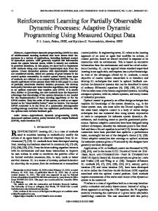
the RL algorithms for smaller datasets from the UCI machine learning repository [7]. The idea of having the agent walk around on these datasets and eat ink pixels is not possible anymore, but we will use a representation that is close in spirit. First of all, an agent receives as state vector three buckets. Each bucket has the same size as the input vector xi . The first bucket B1 is always a copy of xi so that the agent is always allowed to see the actual input. The second bucket B2 is initially set to all 0’s and these 0’s can be set by the agent to copies of elements of the input vector. The third bucket B3 is initially set to a copy of the input vector and these inputs can be set to 0’s by actions of the agent. This means therefore that the length of the augmented input vector is three times the size of the original input vector. Furthermore, the agent has actions to set the inputs in the last two buckets. For the ‘attend’ bucket B2 there is a separate action for each cell that sets its value to the copy of the input vector at the same place. For the ‘ignore’ bucket B3 there is a separate action for each cell in the bucket and that sets its value 0. Thus the proposed architecture implements a specific dynamic feature attention and selection scheme. Finally the reward function is class independent and is only based on the number of 0’s in the last two buckets. Denote 0 ≤ z ≤ 2m as the number of zeros in the last two buckets. z Then the reward emitted after each action is rt = 1 − m which is therefore between -1 and 1. Although the reward function is class independent, the agent with the same class as a training instance will select actions to maximize its obtained rewards, whereas an agent of another class will select actions that minimize its obtained rewards. x1 x2
x3
x4
x5
0
0
0
0
0
x1
x2 x3
x4 x5
x1 x2
x3
x4
x5
0
x2
0
0
0
x1
x2 x3
x4 x5
Reward = 0.2
x1 x2
x3
x4
x5
0
x2
0
0
0
x1
0
x3
x4 x5
Reward = 0.0
x1 x2
x3
x4
x5
0
x2
x3
0
0
x1
0
x3
x4 x5
Reward = 0.2
Fig. 1: In this example, the original input vector consists of 5 inputs. The agent acts on the last two buckets for a fixed number of steps. If an action has been selected before, it does not have an effect on the bucket cell the second time. Figure 1 shows the framework where an agent interacts with an input vector. Suppose the input vector is an image of a face, then an optimal face agent will make its three buckets full with the same face. Another class agent, suppose a car agent, will empty the last bucket, and therefore will only keep the first bucket with the face and the other buckets will become cleared.
Now we will formally define the specific CMDP we use here: •
•
•
•
•
• •
•
S denotes the state-space. It is usually continuous and for an input vector xi of length m the state si ∈ S has 3m elements. The elements are divided into three buckets. Note that S is determined by the classification dataset. st denotes the state-vector at time t in a single epoch, where an agent works on a single example. A denotes the action-space. There are in total 2m actions that set the respective bucket cells. at denotes the action selected at time-step t. The initial state s0 for an input vector xi is s0 = (xi , ~0, xi ) where the three buckets are all of size m. The input vector xi from which the initial state is constructed is taken iteratively from the dataset. The transition function T is deterministic and copies the previous state and executes the action. If the action satisfies 0 ≤ at < m then the new state st+1 = O(st , at ) where the operator O executes the effect of the action as follows: the (m + at )th bucket cell is set to a copy of the ath t element of the input vector. If the action satisfies m ≤ at < 2m then the new state st+1 = O(st , at ) where the operator O executes the effect of the action as follows: the (m + at )th bucket cell is set to 0. The reward function depends on the number of zeros and z is given by rt = 1 − m where z is the number of zeros in the state-vector. A discount factor γ is used. A maximal number of actions in an epoch is used that denotes the horizon h. A flag is used for training that indicates whether the agent represents the same class as the class of the training instance. This determines whether the agent should maximize or minimize its reward intake.
During the learning process the class agents interact with the training examples, where examples are presented one at a time. Each epoch a new training example is given to a class agent. After that the next class agent receives the same example. They perform a number h of actions on it and learn from the observed transitions and obtained rewards. After a number of epochs is finished, the agents can be tested on unseen testing images. During testing, the agents do not act and therefore do not receive rewards. They have observed the effects of their actions on similar original state-vectors s0 and can immediately compute the value of the new instance. The class agent which has the largest value for this initial state outputs its represented class. Since we are working with continuous, high-dimensional state-spaces, we need to use a function approximator. In our current research we have used a multi-layer perceptron (MLP) [4], [5]. Compared to training a normal MLP with backpropagation [4], testing new instances costs almost the same amount of time. However, during the learning process, all class agents have to interact with the input for h steps. Furthermore, the class agents need to compare the outputs of
all action networks to select actions. Since there are in total 2m action networks, the training process is a factor 2hm slower than conventional backpropagation training. In the discussion we will show extensions that can speed up this process. III. T HE M AX -M IN ACLA A LGORITHM We already noted that we use a single reward function that is independent of the target class. However, during training we want to learn large output values for the agent that represents the correct class for an instance and low values for the agent(s) with a wrong class. Furthermore, during testing we want to have a fast algorithm that only works with the initial state vector and does not need to select actions. For these reasons we use an extension of the Actor-Critic Learning Automaton (ALCA) [3], although we could also have used QV-learning [8] or other actor-critic algorithms [2]. The reason is that these algorithms learn a separate state-value function. We cannot easily use Q-learning [9] or similar algorithms, since they need to select an action. This has two disadvantages: (1) when selecting an action for a test example, it is difficult to do this without knowing the label beforehand, and (2) when the algorithms needs to select an action for test examples, it becomes much slower for classifying new data then just using the state values of the initial state. We will now present ACLA. ACLA uses an agent ACi for each class i. Furthermore, it uses a state value function Vi (·) and different preference P -functions for selecting each action a: Pia (·). For representing these value functions we use multi-layer perceptrons which are trained with backpropagation. After an action is performed, the agent receives the following information: (st , at , rt , st+1 ). The agent computes the temporal difference (TD) error δt [10] as follows. If t < h then: δt = rt + γVi (st+1 ) − Vi (st ) Else if t = h: δt = rt − Vi (st ) A TD-update [10] is made to the value function: Vi (st ) = Vi (st ) + αδt Where α denotes the learning rate of the critic. Then the target value for the actor of the selected action is computed as follows: If δt ≥ 0
G=1
Else If δt < 0
G=0
After which the value G is used as a target for learning the action network Piat (·) on the state-vector st with backpropagation. So far we described the ACLA algorithm and we will now explain the Max-Min ACLA algorithm. The whole idea of learning high values for the right class and low values for the wrong class(es) lies in the used exploration policy. Note that ACLA is an on-policy learning method. Furthermore, its initial state value depends on the actions that change the initial state
and obtain rewards. Now suppose that the agent ACi has to select actions for class y = i during training, so it needs to maximize its reward intake in order to learn high state values. In this case the agent uses the conventional Boltzmann or Softmax exploration policy: a
ePi (st )/τ P (a) = P P b (s )/τ t i be Where τ is the temperature. If the agent ACi has to learn values for another class y 6= i then it selects actions with the Min Boltzmann exploration policy: a
e−Pi (st )/τ P (a) = P −P b (s )/τ t i be In this way, it will try to obtain negative rewards for wrong classes and these negative rewards will then be passed by TDlearning to the value of the initial state. Another option would be to set the value of G as described above to 1 for actions that have negative TD-errors, and to 0 for positive TD-errors. This would result in basically the same algorithm. Finally, for testing purposes we compute all values Vi (s0 ) for all classes i and agents ACi belonging to these classes. The input vector is classified with the predicted class yp belonging to the agent with the largest state value: yp = arg max Vi (s0 ) i
There are several reasons why this set-up is useful. First of all, it allows us to have fast classification of new instances. All that is needed is to compute the state-value functions of the initial state Vi (s0 ) and assign the instance to the agent having the largest state-value. This would not be possible if we would have used a reward function that is class dependent, e.g., one that emits positive rewards when an agent not representing the class of the instance sets bucket cells to 0. In that case, the initial value of this agent could also be very large, and direct comparison of state-values would become impossible. Now it is also clear why we cannot use Q-learning: it needs to select at least one action to get a value. However, for testing examples it is unknown whether the class agents need to select a maximizing or minimizing action. A second advantage of our method is that we can use a single reward function for all datasets that is symmetric around 0. We experimented with some different reward functions, but the one we use now seems to work best. IV. E XPERIMENTS In this section the performance of our reinforcement learning method is compared to a conventional multi-layer perceptron (MLP) and a support vector machine (SVM). For this we use 8 datasets from the UCI repository shown in Table I. We will report the results with average accuracy and standard deviations. We use 90% of the data for training data and 10% for testing data. We have performed 1000 experiments per method where each time new data-splits are used. Experimental setup. Since the performances of the classifiers depend heavily on the used learning parameters, we used
Dataset Hepatitis Breast Cancer W. Ionosphere Ecoli Glass Pima Indians Votes Iris
#Instances 155 699 351 336 214 768 435 150
#Features 19 9 34 7 9 8 16 4
#Classes 2 2 2 8 7 2 2 3
TABLE I: The 8 datasets from the UCI repository that are used. many experiments to fine-tune these. For all datasets we used N classifiers trained with the one-versus-all method, where N is the number of classes, except for the SVM case with 2 classes, where only 1 classifier is trained. We used a neural network with sigmoid activations in the hidden units and a linear output unit. For the conventional neural network we also used another error function than the normal squared error one. Although we minimize the squared error, the backpropagation algorithm is not used on an instance where the output of the network times the target output is larger than one. So if yi denotes the output of a neural network on instance xi and the correct output is denoted with yc ∈ {−1, 1}, then no update to the weights is made if yi yc > 1. This makes sure we do not constrain the output to an absolute value of one if the output is already correctly predicted and this improved the results of the standard MLP. For the SVM we used RBF kernels and the best values for γ and C were found with grid-search with values C ∈ {2−5 , 2−3 , . . . , 215 } and γ ∈ {2−15 , 2−13 , . . . , 23 }. All inputs were normalized between -1 and 1. To find the learning parameters we computed the average testing accuracy on all available data. After finding the best parameters, we used them to get the average accuracies using 1000 new experiments. This was used with all methods. Dataset Hepatitis Breast Cancer W. Ionosphere Ecoli Glass Pima Indians Votes Iris
#Hidden units 5 8 11 6 6 5 5 4
lr. α 0.009 0.011 0.007 0.003 0.007 0.002 0.006 0.008
#Examples 20000 80000 50000 100000 50000 100000 2500 70000
TABLE II: The best found parameters for the neural network trained with backpropagation. The best learning parameters of the MLP are shown in Table II. Note that we also optimized the number of presented training examples, which works like an early stopping rule. The best found learning parameters for the reinforcement learning method that also uses MLPs are shown in Table III. To decrease the number of learning parameters, we fixed the learning-rate of the actor to be equal to the learning-rate of the critic. Furthermore, the MLP for the state value function and all action preference value functions had the same number of hidden units. Experimental results. The results on the 8 datasets are shown in Table IV. Although the differences in accuracies of
Dataset Hepatitis Breast Cancer W. Ionosphere Ecoli Glass Pima Indians Votes Iris
#hu 4 8 11 7 8 5 6 4
α 0.004 0.005 0.03 0.005 0.005 0.002 0.005 0.03
h 6 6 7 8 8 7 5 6
γ 0.9 0.9 0.9 0.9 0.97 0.9 0.9 0.93
τ 0.04 0.04 0.06 0.06 0.04 0.06 0.06 0.05
#Exams 35000 50000 100000 100000 50000 100000 55000 65000
TABLE III: The best found parameters for the proposed RL method that combines Max-Min ACLA with neural networks.
the three methods are not large, the reinforcement learning method is able to achieve a higher average accuracy than the normal MLP. Furthermore it wins on 2 datasets against the MLP and loses only on one dataset. Against the SVM, the RL method wins 2 times and loses on 2 datasets. Dataset Hepatitis Breast Cancer W. Ionosphere Ecoli Glass Pima Indians Votes Iris Average Wins/Losses
MLP 84.3 ± 8.6 97.0 ± 1.9 91.1 ± 4.7− 87.6 ± 5.6+ 64.5 ± 11.2− 77.4 ± 4.6 96.6 ± 2.1 97.8 ± 3.8 87.0 1-2
SVM 81.9 ± 9.6− 96.9 ± 2.0 94.0 ± 2.5+ 87.0 ± 5.6 70.1 ± 10.2+ 77.1 ± 4.5 96.5 ± 2.8 96.5 ± 4.8− 87.5 2-2
RL + MLP 84.3 ± 9.2 96.9 ± 2.0 92.8 ± 4.9 87.0 ± 5.7 66.5 ± 11.0 77.4 ± 4.6 96.6 ± 2.7 97.7 ± 4.3 87.4
TABLE IV: The accuracies on the 8 datasets of a normal MLP, a support vector machine (SVM), and our reinforcement learning method. +/- means significant (p = 0.05) win/loss compared to the RL method. Note that our reinforcement learning algorithm uses much more parameters in total when we also consider the action networks. However, since only the state value functions are used for classification, the number of parameters in the classifier is comparable to the other methods. Although RL methods in general do not overfit for control problems, we noticed that overfitting could happen to our reinforcement learning algorithm when we trained the agents too often on the same examples. To cope with that, we used a maximal number of training epochs. V. D ISCUSSION AND E XTENSIONS In this section we will first answer the research questions and then a number of possible extensions to the proposed method is described. • Question: How can value-function based RL algorithms be used for solving classification tasks? Answer: We have explained a novel framework that can be applied to turn a classification problem into a classification Markov decision process. Furthermore, we have described how the Max-Min ACLA algorithm can be used to solve the MDP modeling the classification problem. • Question: How does this novel approach compare to well known machine learning algorithms such as neural networks and support vector machines?
Answer: The RL method slightly outperforms neural networks while a similar representation is used. The performance is about equal to support vector machines. More experiments need to be performed to compare the different methods to examine on what type of problems the RL approach performs best. • Question: What are the advantages and disadvantages of the proposed approach? Answer: A big advantage is that there are many possible extensions of our approach, basically we opened a whole new line of possible research. Disadvantages of our method are that it needs more learning parameters to tune, and that training time of our current method is much longer than the time to train conventional classifiers. We will now describe a number of extensions to our method. First of all, we can use different function approximators than MLPs. For example, we intend to study the performance of our method when support vector machine regression is used for approximating the value functions. Furthermore, other reinforcement learning algorithms such as the AIXI agent [11], [12], the success-story algorithm [13], [14], or the G¨odel Machine [15] can be used in our framework that have better theoretical properties or need less design constraints. It may also be worthwhile to look at ensembles of reinforcement learning algorithms [16], where ACLA is for example combined with QV-learning and Actor-Critic methods. Speed up of our method. One important improvement that we will make is to increase the speed of action selection. Since for an input vector with length m we have 2m action networks, the algorithm is quite slow for training. This can be considerably improved by different methods: (1) We can use a tree representation where the actions are at the leaves and binary action decision nodes in the tree are trained to select a node or action from the left or right branch. This will make the number of action networks that need to be evaluated log2 m + 1, which is a considerable speed up. Care needs to be taken, however, that this improvement is not at the cost of the accuracy. (2) We can use the CACLA algorithm [17] to output a single action. The CACLA algorithm is a continuous action reinforcement learning algorithm that extends ACLA. When rounding the continuous action to the nearest allowed integer [3], action selection only requires evaluating 1 action network. Continuous mental representations. Another extension is the use of more complicated buckets. In principle any kind of memory can be used, e.g., a 2D grid where elements interact can be used or actions representing complex operators on the input can also be used. Genetic programming [18], [19] can also be used for making complex mental representations. We will first concentrate on using the CACLA algorithm to set continuous values in the buckets and explore different reward functions to deal not only with zeros, but with arbitrary values. Feature extraction from images with RL. A final possible extension is to use RL agents to extract features from images for image categorization problems such as arising in handwriting, face, and object recognition. Feature extraction for such
problems is very important in order to obtain invariant representations of the input images. Most current approaches deal with this by having particular box-filters or lines in particular directions. These methods can be combined with maximum or averaging operators to compute e.g. translation invariant features. Although they can be used quite successfully for different image recognition problems, they are quite static. Instead, reinforcement learning agents can be put at particular positions in a grid and can learn to compute particular values describing features around that point in the image. Such agents could learn to navigate to find particular curvatures of orientation gradients, or could focus on finding particular colorful object-parts. Applying RL for feature extraction might play an important role for adding attention to particular elements in an image, and would be very interesting to study as well. Such agents could be part of the current proposed framework, but could also only be applied for feature extraction after which conventional machine learning algorithms can be used to train classifiers mapping the extracted features to class labels. VI. C ONCLUSION A novel framework is described in this paper that allows RL algorithms to train classifiers. Instead of minimizing a particular loss function to adjust the parameters of some classifier, a value-function based RL agent learns value functions from its interaction with the input. There are many possible extensions of the basic approach described in this paper. Next to evaluating these extensions, we want to have a better theoretical understanding of the utility of using RL algorithms to solve classification problems. The current method does not directly use the created mental representations of the input and we will examine whether this would not give better performances, especially when more complex mental representations can be formed. It will also be interesting to combine the RL method with SVM regression that may lead to an improved generalization power. We also want to speed up the proposed algorithm to enable applying it to text, face, and object recognition datasets. For these applications, we also want to focus on RL methods that learn to extract informative features from the images. This can be done by letting the agents search for information in an image and output values that describe the contents of visited regions in the images.
R EFERENCES [1] L. P. Kaelbling, M. L. Littman, and A. W. Moore, “Reinforcement learning: A survey,” Journal of Artificial Intelligence Research, vol. 4, pp. 237–285, 1996. [2] R. S. Sutton and A. G. Barto, Reinforcement Learning: An Introduction. The MIT press, Cambridge MA, A Bradford Book, 1998. [3] H. van Hasselt and M. Wiering, “Using continuous action spaces to solve discrete problems,” in Proceedings of the International Joint Conference on Neural Networks (IJCNN 2009), 2009, pp. 1149–1156. [4] P. J. Werbos, “Advanced forecasting methods for global crisis warning and models of intelligence,” in General Systems, vol. XXII, 1977, pp. 25–38. [5] D. E. Rumelhart, G. E. Hinton, and R. J. Williams, “Learning internal representations by error propagation,” in Parallel Distributed Processing. MIT Press, 1986, vol. 1, pp. 318–362. [6] V. Vapnik, The Nature of Statistical Learning Theory. Springer-Verlag, 1995. [7] C. Blake, D. Newman, and C. Merz, “UCI repository of machine learning databases,” 1998. [Online]. Available: http://www.ics.uci.edu/∼mlearn/MLRepository.html [8] M. Wiering and H. van Hasselt, “Two novel on-policy reinforcement learning algorithms based on TD(λ)-methods,” in Proceedings of the IEEE International Symposium on Adaptive Dynamic Programming and Reinforcement Learning, 2007, pp. 280–287. [9] C. J. C. H. Watkins, “Learning from delayed rewards,” Ph.D. dissertation, King’s College, Cambridge, England, 1989. [10] R. S. Sutton, “Learning to predict by the methods of temporal differences,” Machine Learning, vol. 3, pp. 9–44, 1988. [11] M. Hutter, Universal Artificial Intelligence: Sequential Decisions based on Algorithmic Probability. Berlin: Springer, 2004. [12] J. Poland and M. Hutter, “Universal learning of repeated matrix games,” in Proceedings of the 15th Annual Machine Learning Conference of Belgium and The Netherlands (Benelearn’06), Ghent, 2006, pp. 7–14. [13] J. Schmidhuber, J. Zhao, and N. Schraudolph, “Reinforcement learning with self-modifying policies,” in Learning to learn, S. Thrun and L. Pratt, Eds. Kluwer, 1997, pp. 293–309. [14] J. Schmidhuber, J. Zhao, and M. Wiering, “Shifting inductive bias with success-story algorithm, adaptive levin search, and incremental selfimprovement,” Machine Learning, vol. 28, pp. 105–130, 1997. [15] J. Schmidhuber, “Ultimate cognition a` la G¨odel,” Cognitive Computation, vol. 1, pp. 177–193, 2009. [16] M. Wiering and H. van Hasselt, “Ensemble algorithms in reinforcement learning,” IEEE Transactions, SMC Part B, special issue on Adaptive Dynamic Programming and Reinforcement Learning in Feedback Control, 2008. [17] H. van Hasselt and M. Wiering, “Reinforcement learning in continuous action spaces,” in Proceedings of the IEEE International Symposium on Adaptive Dynamic Programming and Reinforcement Learning (ADPRL 2007), 2007, pp. 272–279. [18] J. H. Schmidhuber, “Evolutionary principles in self-referential learning, or on learning how to learn: the meta-meta-... hook. Institut f¨ur Informatik, Technische Universit¨at M¨unchen,” 1987. [19] J. R. Koza, Genetic Programming II – Automatic Discovery of Reusable Programs. MIT Press, 1994.