Reinforcement Learning and Beyond Part III Multi

1

AAMAS09 Tutorial: Reinforcement Learning and Beyond Part III Multi-agent Learning and Learning Automata

2

Fundamentals of LA Discrete Automata Continuous Automata LA and Reinforcement Learning Fundamentals of Game Theory and MARL Traditional Game Theory Evolutionary Game Theory Learning Automata and Games ESRL

3

Limitations of Game Theory and Possible Solutions A little game Limitations of game theory Overcoming the limitations (and the relevance to MAS)

Katja Verbeeck, Steven de Jong, Peter Vrancx

4

Learning Automata for Human-inspired Fairness in MAS Human-inspired fairness Behavioral economics: social dilemmas, human mechanisms The relevance to MAS (2)

Information Technology, KaHo-Sint Lieven Ghent, KUL, Belgium Micc, University of Maastricht, The Netherlands COMO, Vrije Universiteit Brussel, Belgium with special thanks to Ann Nowé and Karl Tuyls

Human-inspired utility models Applying learning automata Case study: Solving the social dilemma

5

Multi-state LA algorithms LA learning in MDPs

May, 11th 2009

LA learning in Markov Games Optimality in MMDPs Homo Egualis learning in Markov Games

6

1

2

Fundamentals of LA Discrete Automata Continuous Automata LA and Reinforcement Learning Fundamentals of Game Theory and MARL Traditional Game Theory Evolutionary Game Theory Learning Automata and Games ESRL

3

Limitations of Game Theory and Possible Solutions A little game Limitations of game theory Overcoming the limitations (and the relevance to MAS)

4

Learning Automata for Human-inspired Fairness in MAS Human-inspired fairness Behavioral economics: social dilemmas, human mechanisms The relevance to MAS (2) Human-inspired utility models Applying learning automata Case study: Solving the social dilemma

5

Multi-state LA algorithms LA learning in MDPs LA learning in Markov Games Optimality in MMDPs Homo Egualis learning in Markov Games

6

Conclusion

Conclusion

2 dimensions

A Qualitative Definition

A Qualitative Definition

Definition A fusion of the work of psychologists in modeling observed behavior (stimulus-response theory of Estes (1959)), the efforts of statisticians to model the choice of experiments based on past observations, the attempts of operation researchers to implement optimal strategies in the context of the 2-armed bandit problem and the endeavors of systems theorists to make rational decisions in random environments.

Definition Simple decision Making Devices A finite number of actions can be performed in a random environment. When a specific action is performed the environment provides a random response which is either favorable or unfavorable. The objective in the design of the automaton is to determine how the choice of the action at any stage should be guided by past actions and responses. The important point to note here is that the decisions must be made with little knowledge concerning the nature of the environment.

Narendra, K. and Thathachar, M.A.L, Learning Automata: An Introduction, Prentice-Hall International, Inc 1989

A Formal Definition: The Environment

Stationarity vs Non-stationarity

Definition Actions A = {a1 , a2 , . . . , al }

-

c = {c1 , c2 , . . . , cl }

Outputs b = {0, 1}

-

An environment is stationary when, corresponding to each action the probability of obtaining a favorable response is independent of time. Types of Non-stationarity: 1

b = 0 identifies a favorable response or succes, b = 1 identifies a failure

Pr (b(n) = 1|a(n) = ai ) = ci (i = 1, . . . , l)

2

ci (n) is periodic ci (n) is slow-varying

3

ci (n) is a random variable that depends on the actions of the automaton

4

multi-automata environment: changes in the actions chosen by other automata

A Formal Definition: The Automaton

Example: A deterministic automaton

b=0 Transition Function: F : ψ × B → ψ Input Set B

 c ? c ψ1 ψ2 

 -c c ? ψ3 ψ4 

Output Set A

B = {b1 , b2 } -

The State: ψ = {ψ1 , ψ2 , . . . , ψs }

A = {a1 , a2 , . . . , al } -

c -c ψ1 ψ2 

b=1

Output Function: G : ψ → a a deterministic automaton: F and G are deterministic a stochastic automaton: F or G are stochastic

State and Action Probabilities The output function can always be made deterministic by redefining ˆij = (ψi , aj ) the states as tuples ψ → It is just a matter of knowing the probability with which the automaton is in a particular state at a given moment.



1 0  1 0 F (0) =   0 0 0 0

0 0 0 0

  0   0  F (1) =   1  1

0 0 0 0

 c ψ3  1 0 1 0

0 1 0 1

c ψ4

  0   0  G=  0  0

1 1 0 0

 0 0   1  1

State and Action Probabilities The output function can always be made deterministic by redefining ˆij = (ψi , aj ) the states as tuples ψ → It is just a matter of knowing the probability with which the automaton is in a particular state at a given moment.

αj (0) ≡ Pr {ψ (0) = ψj } αj (n) ≡ Pr {ψ (n) = ψj |b(0), . . . , b(n − 1)} α (n)

= F T (b(n − 1))F T (b(n − 2)) . . . F T (b(0))α (0)

Using the action probability vector p(n) with pi (n) = Pr {a(n) = ai |b(0), . . . , b(n − 1)} we get:

p(n) = GT α (n)

State and Action Probabilities The output function can always be made deterministic by redefining ˆij = (ψi , aj ) the states as tuples ψ → It is just a matter of knowing the probability with which the automaton is in a particular state at a given moment.

αj (0) ≡ Pr {ψ (0) = ψj } αj (n) ≡ Pr {ψ (n) = ψj |b(0), . . . , b(n − 1)} α (n)

= F T (b(n − 1))F T (b(n − 2)) . . . F T (b(0))α (0)

Using the action probability vector p(n) with pi (n) = Pr {a(n) = ai |b(0), . . . , b(n − 1)} we get:

p(n) = GT α (n)

Deterministic vs Fixed vs Variable Structure Automata

(Narendra, Thathachar 1989) Consider the case where you have to choose between 2 restaurants-Simeone’s and Delmonaco’s. Let us assume that at stage (n-1) you chose to go to Simeone’s. If your decision at stage n, is to return to Simeone’s if the food was good at stage (n-1), and to switch to Delmonaco’s if it was poor, then your decision corresponds to that of a deterministic automaton. If your decision is to go to the same restaurant if the food was good on the previous visit, but to toss a coin to choose which of the two restaurants to visit if it was not, then you are acting like a fixed structure automaton. Finally, if you update the probs of going to the two restaurants at every stage based on the outcome of the previous visit your decision rule corresponds to a variable-structure automaton.

→ Given a deterministic input sequence, action probabilities can be calculated!

Random inputs and Variable structure Automata

Norms of Behavior Average penalty : M(n)

= Σli =1 ci pi (n)

The action probability vector describes a continous state, discrete-time, Markov process on the l-dimensional simplex: {p|Σli =1 pi = 1; 0 ≤ pi ≤ 1} and when p(n + 1) depends on p(n) but not explicitely on n, {p(n)}n>=0 is a homogenous Markov process.

= E[b(n) = 1|p(n)] = Σli =1 [b(n) = 1|a(n) = ai ]

For the pure-chance automaton M(n) = M0 = n1 Σli =1 ci A learning automaton is said to be: 1 2 3 4

expedient if limn→∞ E[M(n)] < M0 optimal if limn→∞ E[M(n)] = mini ci

ε -optimal if limn→∞ E[M(n)] < mini ci + ε absolutely expedient if E[M(n + 1)|p(n)] < M(n)

L2,2 , Tsetlin, 1961

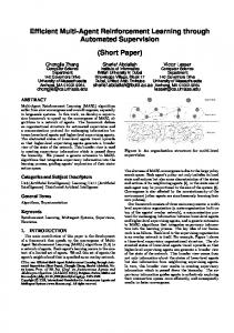
Behavior of L2,2

Performs whatever action it was using earlier as long as the response is positive, but changes to the other action otherwise. The resulting Markov chain is ergodic, the limiting probabilities are:

b=0

 ? c ψ1 , a1 

α1 =

 c ? ψ2 ,a2

c1 c2 , α2 = c1 + c2 c1 + c2

and thus L2,2 is expedient (c1 6= c2 ), M(L2,2 ) =

b=1

ψ1 ,a1

c  

2c1 c2 c + c2 < M0 = 1 c1 + c2 2

 c ψ2 ,a2 

Adding Memory, L2N,2 , Tsetlin

Variable Structure Automata

Keeps an account of the number of successes and failures and when the number of failures exceeds a number N, it switches the action. 1 2

b=0

a2

a1

 ? c 1 

2

c

N

c

c

2N

-c

c

N +2

 -c ? N + 1

3 4 5

a1

c

b=1

If mini {ci } ≤

1 2

1

-c 2

 -  c c N 2N

a2

c

c

N +2

c

N +1

then limN→∞ M(L2N,2 ) = min(c1 , c2 ) (conditionally ε -optimal)

evolve action probabilities (or equiv state probs) assume each state corresponds to one distinct action ((G ) is the identity mapping) analyzing tool: discrete-time Markov processes {p(n)}n define a mapping T so that : p(n + 1) = T [p(n), a(n), b(n)] characteristics: asymptotic behavior: expedient, (ε -)optimal nature of the mapping: lineair, nonlineair, hybrid properties of the Markov process: ergodic, nonergodic

Reward-Penalty with binary feedback

b=0

  pi (t + 1) = 

b=1

pj (t + 1) =

pi (t) + λ1 (1 − pi (t))

if action i was taken at time step t

(1 − λ1 )pj (t) ∀j 6= i

 pi (t + 1) = pi (t) − λ2 pi (t)   

if action i was taken at time step t

  

pj (t + 1) = pj (t) + λ2 [(l − 1)−1 − pj (t)] ∀j 6= i

λ1 , λ2 ∈]0, 1[ and l the number of actions. λ1 = Reward parameter and λ2 = penalty parameter λ1 = λ2 : linear reward-penalty (LR−P ) , λ2 = 0 : linear reward-inaction (LR−I ), λ2