Sensors 2009, 9, 148-174; doi:10.3390/s90100148 OPEN ACCESS
sensors ISSN 1424-8220 www.mdpi.com/journal/sensors Article
Remote Sensing Data with the Conditional Latin Hypercube Sampling and Geostatistical Approach to Delineate Landscape Changes Induced by Large Chronological Physical Disturbances Yu-Pin Lin *, Hone-Jay Chu, Cheng-Long Wang, Hsiao-Hsuan Yu and Yung-Chieh Wang Department of Bioenvironmental Systems Engineering, National Taiwan University, 1, Sec. 4, Roosevelt Rd., Da-an District, Taipei City 106, Taiwan, R. O. C; E-Mails:
[email protected] (H.-J. C.);
[email protected] (C.-L. W.);
[email protected] (H.-H. Y.);
[email protected] (Y.-C. W.) * Author to whom correspondence should be addressed; Email:
[email protected] (Y.-P. L.); Tel.: +886-2-33663467; Fax: +886-2-33663464 Received: 12 November 2008; in revised form: 5 January 2009 / Accepted: 6 January 2009 / Published: 7 January 2009
Abstract: This study applies variogram analyses of normalized difference vegetation index (NDVI) images derived from SPOT HRV images obtained before and after the ChiChi earthquake in the Chenyulan watershed, Taiwan, as well as images after four large typhoons, to delineate the spatial patterns, spatial structures and spatial variability of landscapes caused by these large disturbances. The conditional Latin hypercube sampling approach was applied to select samples from multiple NDVI images. Kriging and sequential Gaussian simulation with sufficient samples were then used to generate maps of NDVI images. The variography of NDVI image results demonstrate that spatial patterns of disturbed landscapes were successfully delineated by variogram analysis in study areas. The high-magnitude Chi-Chi earthquake created spatial landscape variations in the study area. After the earthquake, the cumulative impacts of typhoons on landscape patterns depended on the magnitudes and paths of typhoons, but were not always evident in the spatiotemporal variability of landscapes in the study area. The statistics and spatial structures of multiple NDVI images were captured by 3,000 samples from 62,500 grids in the NDVI images. Kriging and sequential Gaussian simulation with the 3,000 samples effectively reproduced spatial patterns of NDVI images. However, the proposed approach, which integrates the conditional Latin hypercube sampling approach, variogram, kriging and sequential Gaussian simulation in remotely sensed images, efficiently monitors,
Sensors 2009, 9
149
samples and maps the effects of large chronological disturbances on spatial characteristics of landscape changes including spatial variability and heterogeneity. Keywords: Chi-Chi earthquake, typhoons, landscape changes, remotely sensed images, geostatistics, spatial patterns, Latin hypercube sampling, conditional simulation.
1. Introduction The influences of large physical disturbances on ecosystem structure and function have garnered considerable attention [1-4]. Fires, hurricanes (typhoons), tornados, ice storms, and landslides are examples of such large disturbances [4]. Earthquakes have long been recognized as a major cause of landslides [5, 6]. However, landslides are only the first in a series of processes by which materials are removed from slopes and transported out of a region by fluvial action [6, 7]. Additionally, typhoons are extremely important natural disturbances that characterize the structure, function and dynamics of many tropical and temperate forest ecosystems [8]. Taiwan, which is located in a subtropical region, sits on the Philippine plate at the Euro-Asian Plate junction [9]. Plate convergence occasionally generates earthquakes that have disastrous effects on Taiwan [10]. Moreover, typhoons that bring tremendous amounts of rainfall hit Taiwan every year from July to October [11]. During 1996–2004, large disturbances in the following sequence impacted central Taiwan: (1) typhoon Herb (August 1996); (2) the Chi-Chi earthquake (September 1999); (3) typhoon Xangsane (November 2000); (4) typhoon Toraji (July 2001); (4) typhoon Dujuan (September, 2003); and, (5) typhoon Mindulle (June 2004) [11]. In particular, after the ChiChi earthquake, the expansion rate of landslide areas increased 20-fold in central Taiwan [12]. Numerous extension cracks, which accelerate landslides during downpours, were generated on hill slopes during the ChiChi earthquake [13]. Moreover, during typhoon seasons, a massive amount of loose earth and stones accumulated on the surface of slopes, increasing the risk of debris flows and additional landslides [14] that worsen the revegetation problem. Accordingly, monitoring, delineating and sampling landscape changes, spatial structure and spatial variation induced by large physical disturbances are essential to landscape management and restoration, and disaster management in Taiwan. Remotely sensed data can describe surface processes, including landscape dynamics, as such data provide frequent spatial estimates of key earth surface variables [15, 16]. For example, the SPOT, LANSAT and MODIS data sets have notable advantages that account for their use in ecological applications, including a long-running historical time-series, a special resolution appropriate to regional land-cover and land-use change investigations, and a spectral coverage appropriate to studies of vegetation properties [17-19]. The Normalized Difference Vegetation Index (NDVI), a widely used vegetation index, is typically used to quantify landscape dynamics, including vegetation cover and landslides changes induced by large disturbances [6, 8, 11, 16, 20]. Notably, NDVI images can be determined by simply geometric operations near-infrared and visible-red spectral data almost immediately after remotely sensed data is obtained. The NDVI, which is the most common vegetation index, has been extensively used to determine the vigor of plants as a surrogate measure of canopy
Sensors 2009, 9
150
density [21]. A high NDVI indicates a high level of photosynthetic activity [22]. Moreover, significant differences in NDVI images before and after a natural disturbance can represent landscape changes, including vegetation and landslides induced by a disturbance that changes plant-covered land to bare lands or bare lands to plant-covered land [23]. Spatial patterns in ecological systems are the result of an interaction among dynamic processes operating across abroad range of spatial and temporal scales [24-26]. Ecological manifestations of large disturbances are rarely homogeneous in their spatial coverage [4]. Variograms are crucial to geostatistics. A variogram is a function related to the variance to spatial separation and provides a concise description of the scale and pattern of spatial variability [27]. Samples of remotely sensed data (e.g., satellite or air-borne sensor imagery) can be employed to construct variograms for remotely sensed research [27]. Moreover, variograms have been used widely to understand the nature and causes of spatial variation within an image [28]. Modeling the variogram of NDVI images with high spatial resolution is an efficient approach for characterizing and quantifying heterogeneous spatial components (spatial variability and spatial structure) of a landscape and the spatial heterogeneity of vegetation cover at the landscape level [28, 29]. Reliable data analysis of spatially distributed data requires the use of appropriate statistical tools and a sound data sampling strategy [30]. Spatial sampling schemes have been developed to determine the sampling locations that cover the variation in environmental properties in a given area [31]. Moreover, data samples are transformed via a series of interpretation steps to obtain complete descriptions of phenomena of interest [32]. Different sampling schemes are, say, random, systematic, stratified, or nested schemes [32, 33]. Latin hypercube sampling (LHS) is a stratified random procedure that is an efficient way of sampling variables from their multivariate distributions [34]. Initially developed for Monte-Carlo simulation, LHS efficiently selects input variables for computer models [35, 36]. Kriging, a geostatistical method, is a linear interpolation approach that provides a best linear unbiased estimator (BLUE) for quantities that vary spatially [37]. However, kriging interpolate algorithms generate maps of best local estimate and generally smooth out the local details of the spatial variation of an attribute [38].For sampled data, a geostatistical conditional simulation technique, such as sequential Gaussian simulation (SGS), can be applied to generate multiple realizations, including an error component, which is absent from classical interpolation approaches [37]. In such conditional simulations, all generated realizations reproduce available data at measurement locations, and, on average, reproduce a data histogram and a model of spatial correlations (i.e., variogram) between observations [39]. In SGS, Gaussian transformation of available measurements is simulated, such that each simulated value is conditional on original data and all previously simulated values [37, 40]. Geostatistical conditional simulations have been widely applied to simulate the spatial variability and spatial distribution of interest in many fields. Moreover, geostatistical simulation techniques with LHS have been applied to simulate Gaussian random fields [39, 41-43]. This study applied variogram analysis to delineate spatial variations of NDVI images before and after large physical disturbances in central Taiwan. The NDVI data derived from SPOT images before and after the ChiChi earthquake (ML=7.3 on the Richter scale) in the Chenyulan basin, Taiwan, as well as images before and after four large typhoons (Xangsane, Toraji, Dujuan and Mindulle) were analyzed to identify the spatial patterns of landscapes caused by these major disturbances. Landscape spatial patterns of different disturbance regimes were discussed. Moreover, conditional LHS (cLHS)
Sensors 2009, 9
151
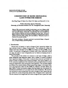
schemes with NDVI images were used to select spatial samples from actual NDVI images to detect landscape changes induced by a series of large disturbances. The best cLHS samples selected with the NDVI values were used to estimate and simulate NDVI distributions using kriging and SGS. The simulated NDVI images were compared with actual NDVI images induced by the disturbances. 2. Methods and Materials 2.1. Study area and remote sensing data The Chenyulan watershed, located in central Taiwan, is a classical intermountain watershed, and has an average altitude of 1,540 m and an area of 449 km2 (Figure 1). The Chenyulan stream, which coincides with the Chenyulan fault, flows from south to north and elongates the watershed in the same direction. Differences in uplifting along the fault generated abundant fractures over the watershed and resulted in an average slope of 62.5% and relief of 585 m/km2. Moreover, the main course of the Chenyulan stream had a gradient of 6.1%, and more than 60% of its tributaries had gradients exceeding 20%. The special geological and geographical characteristics of the watershed result in frequent landsides and debris flows [12]. The September 21, 1999, Chi-Chi earthquake occurred at 1:47 a.m. local time (17:47:18 GMT the previous day) at an epicentral location of 23.85_N and 120.78_E and at a depth 6.99 km (Figure 1). It was caused by a rupture in the Chelungpu Fault. The magnitude of the earthquake was estimated to be ML = 7.3 (ML: Local Magnitude or Richter Magnitude), and the rupture zone, defined by the aftershocks, measured about 80 km north-south by 25–30 km downdip [10, 44]. Iso-contour maps of the earthquake’s magnitude were reproduced from the Central Weather Bureau (Figure 1) [45]. After the earthquake, from October 31, 2000 to November 1, 2000, the center of typhoon Xiangsane moved from south to north through eastern Taiwan [46], with a maximum wind speed of 138.9 km/hr and a radius of 250 km (Figure 1). The maximum daily rainfall was 550 mm/day. On July 30, 2001, the Toraji typhoon swept across central Taiwan from east to west [47], with a maximum wind speed of 138.9 km/hr and a radius of 180 km (Figure 1). The typhoon brought extremely heavy rainfall, from 230 to 650 mm/ day, and triggered more than 6000 landslides in Taiwan. After crossing Taiwan, typhoon Toraji became a tropical storm; however it brought 339 to 757 mm of total accumulated rainfall in the watershed [47] (Figure 1). After typhoon Toraji, typhoons Dujuan with a maximum wind speed of 165.0 km/hr, a radius of 200 km and maximum rainfall 200 mm/hr (August 31, 2003–September 2, 2003) and Mindulle with maximum wind speed of 200.0 km/hr, a radius of 200 km and maximum rainfall 166 mm/hr (June 29, 2004–July 2, 2004) chronologically produced heavy rainfall that fell across the eastern and central parts of Taiwan on September 2003 and June 2004 [48] (Figure 1). The two study area with dimensions of 2 50×50 km (250×250 pixels) was selected from the upstream of the large debris flood announced in the watershed, as shown in Figure 1.
Sensors 2009, 9
152 Figure 1. Location of the study areas.
2.2. NDVI Seven cloud-free SPOT images (1996/11/08, 1999/03/06, 1999/10/31, 2000/11/27, 2001/11/20, 2003/12/17 and 2004/11/19) of the Chenyulan watershed were purchased from the Space and Remotesensing Research Center, Taiwan. The NDVI images of the study area were generated from SPOT HRV images with a resolution of 20 m according to the following equation:
NDVI
NIR R NIR R
(1)
where NIR and R are near-infrared and visible-red spectral data, respectively. The NDVI values range from 1 to 1 ; a high NDVI value represents a large amount of high photosynthesizing vegetation [49].
2.3. Variogram and kriging estimation In geostatistical methods, variograms can be used to quantify the observed relationship between the values of samples and the proximity of samples [37]. Following the work of Garrigues et al. (2006), Garrigues et al. (2008) and Lin et al. (2008), NDVI data are considered values of punctual regionalized variable. An experimental variogram for interval lag distance class h, γ(h) , is represented by 1 n( h) ( h) [ Z ( xi h) Z ( xi )]2 (2) 2n(h) i 1 where h is the lag distance that separates pairs of points; Z(x) is bird diversity at location x, and Z(x + h) is bird diversity at location x + h; n(h) is the number of pairs separated by lag distance h.
Sensors 2009, 9
153
Kriging is estimated using weighted sums of adjacent sampled concentrations. The weights depend on the correlation structure exhibited. The weights are determined by minimizing estimated variance. In this context, kriging estimates (Best Linear Unbiased Estimator) are the most accurate of all linear estimators. Accordingly, kriging estimates the value of the random variable at unsampled location X0 based on measured values in a linear form: N
Z * ( x 0 ) i 0 Z ( x i )
(3)
i 1
where Z*(x0) is the estimated value at location x0, λi0 is the estimation weight of Z(xi), xi is the location of sampling point for variable Z, and N is the number of the variable Z involved in the estimation. Based on non-biased constraints and minimizing estimation variance, estimated kriging variance can be presented as: N
2 kriging i 0 zz ( xi x0 )
(4)
i 1
where µ is the Lagrange multiplier. 2.4. Conditional Latin hypercube The cLHS, which is based on the empirical distribution of original data, provides a full coverage of range each variable by maximally stratifying the marginal distribution and ensuring a good spread of sampling points [34]. This sampling procedure represents an optimization problem: given N sites with ancillary data (Z), select n sample sites (n