Replication Strategies in Unstructured Peer-to-Peer Networks Edith Cohen
Scott Shenker
AT&T Labs–Research 180 Park Avenue Florham Park, NJ 07932, USA
ICSI Berkeley, CA 94704 USA
[email protected]
[email protected]
ABSTRACT The Peer-to-Peer (P2P) architectures that are most prevalent in today’s Internet are decentralized and unstructured. Search is blind in that it is independent of the query and is thus not more effective than probing randomly chosen peers. One technique to improve the effectiveness of blind search is to proactively replicate data. We evaluate and compare different replication strategies and reveal interesting structure: Two very common but very different replication strategies – uniform and proportional – yield the same average performance on successful queries, and are in fact worse than any replication strategy which lies between them. The optimal strategy lies between the two and can be achieved by simple distributed algorithms. These fundamental results offer a new understanding of replication and show that currently deployed replication strategies are far from optimal and that optimal replication is attainable by protocols that resemble existing ones in simplicity and operation.
Categories and Subject Descriptors C.2 [Communication Networks]; H.3 [Information Storage and Retrieval]; F.2 [Analysis of Algorithms]
General Terms Algorithms
Keywords replication; peer-to-peer; random search
1.
INTRODUCTION
Peer-to-peer (P2P) systems, almost unheard of three years ago, are now one of the most popular Internet applications and a very significant source of Internet traffic. While Napster’s recent legal troubles may lead to its demise, there are
Permission to make digital or hard copies of all or part of this work for personal or classroom use is granted without fee provided that copies are not made or distributed for profit or commercial advantage and that copies bear this notice and the full citation on the first page. To copy otherwise, to republish, to post on servers or to redistribute to lists, requires prior specific permission and/or a fee. SIGCOMM’02, August 19-23, 2002, Pittsburgh, Pennsylvania, USA. Copyright 2002 ACM 1-58113-570-X/02/0008 ...$5.00.
many other P2P systems that are continuing their meteoric growth. Despite their growing importance, the performance of P2P systems is not yet well understood. P2P systems were classified by [9] into three different categories. Some P2P systems, such as Napster [6], are centralized in that they have a central directory server to which users can submit queries (or searches). Other P2P systems are decentralized and have no central server; the hosts form an ad hoc network among themselves and send their queries to their peers. Of these decentralized designs, some are structured in that they have close coupling between the P2P network topology and the location of data; see [12, 10, 11, 15, 2] for a sampling of these designs. Other decentralized P2P systems, such as Gnutella [3] and FastTrack [13]based Morpheus [5] and KaZaA [4], are unstructured with no coupling between topology and data location. Each of these design styles – centralized, decentralized structured, and decentralized unstructured – have their advantages and disadvantages and it is not our intent to advocate for a particular choice among them. However, the decentralized unstructured systems are the most commonly used in today’s Internet. They also raise an important performance issue – how to replicate data in such systems – and that performance issue is the subject of this paper. In these decentralized unstructured P2P systems, the hosts form a P2P overlay network; each host has a set of “neighbors” that are chosen when it joins the network. A host sends its query (e.g., searching for a particular file) to other hosts in the network; Gnutella uses a flooding algorithm to propagate the query, but many other query-propagation approaches are possible. The fundamental point is that in these unstructured systems, because the P2P network topology is unrelated to the location of data, the set of nodes receiving a particular query is unrelated to the content of the query. A host doesn’t have any information about which other hosts may best be able to resolve the query. Thus, these “blind” search probes can not be on average more effective than probing random nodes. Indeed, simulations in [9] suggest that random probing is a reasonable model for search performance in these decentralized unstructured P2P systems. To improve system performance, one wants to minimize the number of hosts that have to be probed before the query is resolved. One way to do this is to replicate the data on several hosts.1 That is, either when the data is originally 1 For the basic questions we address, it does not matter if the actual data is replicated or if only pointers to the data
stored or when it is the subject of a later search, the data can be proactively replicated on other hosts. Gnutella does not support proactive replication, but at least part of the current success of FastTrack-based P2P networks can be attributed to replication: FastTrack designates high-bandwidth nodes as search-hubs (super-nodes). Each supernode replicates the index of several other peers. As a result, each FastTrack search probe emulates several Gnutella probes and thus is much more effective. It is clear that blind search is more effective when a larger index can be viewed per probe, but even though FastTrack increased per-probe capacity, it basically uses the same replication strategy as Gnutella: The relative index capacity dedicated to each item is proportional to the number of peers that have copies. Thus, current approaches to replication are largely implicit. We consider the case where one designs an explicit replication strategy. The fundamental question we address in our paper is: given fixed constraints on per-probe capacity, what is the optimal way to replicate data?2 We define replication strategies that, given a query frequency distribution, specify for each item the number of copies made. The main metric we consider is the performance on successful queries, which we measure by the resulting expected (or average) search size A. We also consider performance on insoluble queries, which is captured by the maximum search size allowed by the system. Our analysis reveals several surprising fundamental results. We first consider two natural but very different replication strategies: Uniform and Proportional. The Uniform strategy, replicating everything equally, appears naive, whereas the Proportional strategy, where more popular items are more replicated, is designed to perform better. However, we show that the two replication strategies have the same expected search size on successful queries. Furthermore, we show that the Uniform and Proportional strategies constitute two extreme points of a large family of strategies which lie “between” the two and that any other strategy in this family has better expected search size. We then show that one of the strategies in this family, Square-root replication, minimizes the expected search size on successful queries. Proportional and Uniform replications, however, are not equivalent. Proportional makes popular items easier to find and less popular items harder to find. In particular, Proportional replication requires a much higher limit on the maximum search size while Uniform minimizes this limit and, thus, minimizes resources consumed on processing insoluble queries. We show that the maximum search size with Square-root strategy is in-between the two (though closer to Uniform), and define a range of optimal strategies that balance the processing of soluble and insoluble queries. Interestingly, these optimal strategies lie “between” Uniform and Square-root and are “far” from Proportional. Last, we address how to implement these replication strategies in the distributed setting of an unstructured P2P network. It is easy to implement the Uniform and Proporare replicated. The actual use depends on the architecture and is orthogonal to the scope of this paper. Thus, in the sequel, “copies” refers to actual copies or pointers. 2 Our analysis assumes adaptive termination mechanism, where the search is stopped once the query is resolved. See [7] for a discussion of a different question related to replication in P2P networks without adaptive termination.
tional replication strategies; for Uniform the system creates a fixed number of copies when the item first enters the system, for Proportional the system creates a fixed number of copies every time the item is queried. What isn’t clear is how to implement the Square-root replication policy in a distributed fashion. We present several simple distributed algorithms which produce optimal replication. Surprisingly, one of these algorithms, path replication, is implemented, in a somewhat different form, in the Freenet P2P system. These results are particularly intriguing given that Proportional replication is close to what is used by current P2P networks: With Gnutella there is no proactive replication; if we assume that all copies are the result of previous queries, then the number of copies is proportional to the query rate for that item. Even FastTrack, which uses proactive replication, replicates the complete index of each node at a search hub so the relative representation of each item remains the same. Our results suggest that Proportional, although intuitively appealing, is far from optimal and a simple distributed algorithm which is consistent in spirit with FastTrack replication is able to obtain optimal replication. In the next section we introduce our model and metrics and present a precise statement of the problem. In Section 3 we examine the Uniform and Proportional replication strategies. In Section 4 we show that Square-root replication minimizes the expected search size on soluble queries and provide some comparisons to Proportional and Uniform replication. Section 5 defines the optimal policy parameterized by varying cost of insoluble queries. In Section 6 we present distributed algorithms that yields Square-root replication and present simulation results of its performance.
2. MODEL AND PROBLEM STATEMENT The network consists of n nodes, each with capacity ρ which is the number of copies/keys that the node can hold. 3 Let R = nρ denote the total capacity of the system. There are m distinct data items in the system. The normalized vector of query rates takes the form q = q1 ≥ q2 ≥ · · · ≥ qm qi = 1. The query rate qi is the fraction of all queries with that are issued for the ith item. An allocation is a mapping of items to the number of copies of that item (where we assume there is no more than one copy per node). We let ri denote the number of copies of the i’th item (ri counts all copies, including the original one), and let pi ≡ ri /R be the fraction of the total system m capacity allotted to item i: i=1 ri = R. The allocation is represented by the vector p = (r1 /R, r2 /R, . . . , rm /R). A replication or allocation strategy is a mapping from the query rate distribution q to the allocation p. We assume R ≥ m ≥ ρ because outside of this region the problem is either trivial (if m ≤ ρ the optimal allocation is to have copies of all items on all nodes) or insoluble (if m > R there is no allocation with all items having at least one copy). Our analysis is geared for large values of n (and R = ρn) with our results generally stated in terms of p and ρ with n factored out. Thus, we do not concern ourselves with integrality restrictions on the ri ’s. However, we do care about the bounds on the quantities pi . Since ri ≥ 1, we
P
P
3
Later on in this section we explain how to extend the definitions, results, and metrics to the case where nodes have heterogeneous capacities.
1 have pi ≥ ℓ where ℓ = R . Since there is no reason to have more than one copy of an item on a single node, we have n ri ≤ n and so pi ≤ u where u = R = ρ−1 . Later in this section we will discuss reasons why these bounds may be made more strict. We argued in the introduction that performance of blind search is captured well by random probes. This abstraction allows us to evaluate performance without having to consider the specifics of the overlay structure. Simulations in [9] show that random probes are a reasonable model for several conceivable designs including Gnutella-like overlays. Specifically, the search mechanism we consider is random search: The search repeatedly draws a node uniformly at random and asks for a copy of the item; the search is stopped when the item is found. The search size is the number of nodes drawn until an answer is found. With the random search mechanism, search sizes are random variables drawn from a Geometric distribution with expectation ρ/pi . Thus, performance is determined by how many nodes have copies of any particular item. For a query distribution q and an allocation p, we define the expected search size (ESS) Aq (p) to be the expected number of nodes one needs to visit until an answer to the query is found, averaged over all items. It is not hard to see that
Aq (p) = 1/ρ(
X
qi /pi ) .
(1)
i
The set of legal allocations P is a polyhedron defined by the (m−1)-dimensional simplex of distributions on m items, intersected with an m-dimensional hypercube, which defines upper and lower bounds on the number of copies of each item: m X
pi
=
1
(2)
≤u.
(3)
i=1
ℓ ≤ pi
The legal allocation that minimizes the expected search size is the solution to the optimization problem Minimize
m X i=1
qi /pi such that p ∈ P .
P
fs Aq (p) + (1 − fs )L(p) .
(5)
2.2 Heterogeneous capacities and bandwidth
One obvious property of the optimal solution is monotonicity u ≥ p1 ≥ p2 ≥ · · · ≥ pm ≥ ℓ
Thus, if C = O(log L) then the failure probability would be polynomially small in L. In order to compare two allocations under truncated search, we set the relation between L and ℓ such that the same base set of items is locatable. We now argue that when all m items are locatable, Expression (1) constitutes a close approximation of the expected truncated search size. The distribution of search sizes under truncated random searches is a Geometric distribution with parameter pi , where values greater by L are truncated by L. Thus, Expression (1), which models untruncated search, constitutes an upper bound on the truncated expected search size. The error, however, is at most mini j≥1 (1 − ρpi )L+j = mini (1 − ρpi )L /(ρpi ) ≤ exp(−C)/(ρℓ) = (L/C) exp(−C). In the sequel, we assume that ℓ is such that ℓ > ln L/(ρL) and use the untruncated approximation (1) for the expected search size (it is within an additive term of exp(−ℓρL/ ln L) < 1). Also note that the likelihood for an unsuccessful search for a locatable item is at most exp(−ℓρL) < 1/L. Thus, even though each locatable item can have some failed searches, these searches constitute a very small fraction of total searches for the item. The maximum search size parameter L is also important for analyzing the cost of insoluble queries; that is, queries made to items that are not locatable. In actual systems, some fraction of queries are insoluble, and search performed on such queries would continue until the maximum search size is exceeded. The cost of these queries is not captured by the ESS metric, but is proportional to L and to the fraction of queries that are insoluble. When comparing replication strategies on the same set of locatable items, we need to consider both the ESS, which captures performance on soluble queries and L, which captures performance on insoluble queries. In this situation we assume that the respective L(p) is the solution of mini pi = ln L/(ρL). Thus, if fs is the fraction of queries which are soluble and (1 − fs ) is the fraction of insoluble queries, the performance of the allocation p is
(4)
(If p is not monotone then consider two items i, j with qi > qj and pi < pj . The allocation with pi and pj swapped is legal, if p was legal, and has a lower ESS.) In the next section we explore the performance of two common replication strategies, Uniform and Proportional. However, we first discuss refinements of our basic model.
2.1 Bounded search size and insoluble queries So far we have assumed that searches continue until the item is found, but we now discuss applying these results in a more realistic setting when searches are truncated when some maximal search size L is reached. We say an item is locatable if a search for it is successful with high probability. Evidently, an item is locatable if the fraction of nodes with a copy ρpi is sufficiently large with respect to L. Clearly, truncated searches have some likelihood of failing altogether. The probability of failure is at most 2−C if pi ≥ C/(ρL).
So far we consider a homogeneous setting, where all copies have the same size and all nodes have the same storage and the same likelihood of getting probed. In reality, hosts have different capacities and bandwidth and, in fact, the most recent wave of unstructured P2P networks [5, 4] exploits this asymmetry. For simplicity of presentation we will keep using the homogeneous setting in the sequel, but we note that all out results can be generalized in a fairly straightforward way to heterogeneous systems. Suppose nodes have capacities ρi and visitation weight vi (in the homogeneous case vi = 1, in general vi is the factor in which the visitation rate differs from the average). It is not hard to see that the average capacity seen per probe is ρ = i vi ρi . The quantity ρ simply replaces ρ in Equation 1 and in particular, the ESS of all allocations are affected by the same factor; thus all our findings on the relative performance of different allocations also apply for heterogeneous capacities and visitation rates. An issue that arises when the replication is of copies (rather than pointers) is that items often have very different sizes. Our subsequent analysis can be extended to this case by treating the ith item as a group of ci items with the same
P
query rate, where ci is the size of item i. As a result we obtain altered definitions of the three basic allocations we consider: • Proportional has pi = ci qi / query rate and size). • Uniform has pi = ci / size).
P
j
P
j
cj qj (proportional to
cj (proportional to item’s
P
√ √ • Square-root has pi = ci qi / j cj qj (proportional to size and to the square-root of the query rate).
3.
ALLOCATION STRATEGIES
3.1 Uniform and Proportional We now address the performance of two replication strategies. The Uniform replication strategy is where all items are equally replicated: Definition 3.1. Uniform allocation is defined when ℓ ≤ 1/m ≤ u and has pi = 1/m for all i = 1, . . . , m. This is a very primitive replication strategy, where all items are treated identically even though some items are more popular than others. One wouldn’t, initially, think that such a strategy would produce good results. When there are restriction on the search size (and thus on ℓ), Uniform allocation has the property that it is defined for all q for which some legal allocation exists: Any allocation p other than Uniform must have i where pi > 1/m and j where pj < 1/m; If Uniform results in allocations outside the interval [ℓ, u], then either 1/m > u (and thus pi > u) or 1/m < ℓ (and thus pj < ℓ). An important appeal of the Uniform allocation is that it minimizes the required maximum search size, and thus, minimizes system resources spent on insoluble queries. It follows from Equation (5) that when a large fraction of queries are insoluble, Uniform is (close to) optimal. Another natural replication strategy is to have ri be proportional to the query rate. Definition 3.2. Proportional allocation is defined when ℓ ≤ qi ≤ u. The Proportional solution has pi = qi for all i. Some of the intuitive appeal of Proportional allocation is that it minimizes the maximum utilization rate [9]. This metric is relevant when the replication is of copies rather than of pointers; that is, when a successful probe is much more expensive to process than an unsuccessful probe. The utilization rate of a copy is the average rate of requests it serves. Under random search, all copies of the same item i have the same utilization rate qi /pi ; when there are more copies, each individual copy has a lower utilization. To avoid hot-spots, it is desirable to have low values for the maximum utilization rate of a copy maxi qi /pi . The average utilization over all copies, m i=1 pi qi /pi = 1, is independent of the allocation p. The proportional allocation has qi /pi = 1 for all i, and so it clearly minimizes the maximal value maxi qi /pi . When compared to Uniform, Proportional improves the most common searches at the expense of the rare ones, which presumably would improve overall performance. We now analyze some of the properties of these two strategies. A straightforward calculation reveals the following surprising result:
P
Lemma 3.1. Proportional and Uniform allocations have the same expected search size A = m/ρ, which is independent of the query distribution. We note that Lemma 3.1 easily generalizes to all allocations that are a mix of Proportional and Uniform, in which each item i has pi ∈ {1/m, qi }. We next characterize the space of allocations.
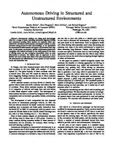
3.2 Characterizing allocations As a warmup, we consider the space of allocations for two items (m = 2). We shall see that Proportional and Uniform constitute two points in this space with anything “between” them achieving better performance, and anything “outside” having worse performance. Consider a pair of items with qi ≥ qj . The range of allocations is defined by a single parameter 0 < x < 1, with pi /(pi + pj ) = x and pj /(pi + pj ) = (1 − x). Proportional corresponds to x = qi /(qi + qj ), and Uniform to x = 0.5. The range 0.5 ≤ x ≤ qi /(qi + qj ) captures allocations “between” Uniform and Proportional. The “outside” range 0 < x < 0.5 contains non-monotone allocations where the less-popular item obtains a larger allocation. The “outside” range 1 > x > qi /(qi + qj ) contains allocations where the relative allocation of the more popular item is larger than its relative query rate. These different allocations are visualized in Figure 1(A), which plots pi /pj as a function of qi /qj . The ESS for these two items is proportional to qi /x + qj /(1 − x). This function has equal value on x = 0.5 and x = qi /(qi + qj ) and is convex. The minimum is obtained at some middle point in the “between” range. By taking the first derivative, equating it to zero, and solving the resulting quadratic equation, we obtain that the minimum is obtained √ √ √ at x = qi /( qi + qj ). Figure 1(B) shows the expected search size when using these allocations on two items (m = 2 and ρ = 1). In this case, the maximum gain factor by using the optimal allocation over Uniform or Proportional is 2. In the sequel we extend the observations made here to arbitrary number of items (m ≥ 2). In particular, we develop a notion of an allocation being “between” Uniform and Proportional and show that these allocations have better ESS, and that “outside” allocations have worse ESS. We also define the policy that minimizes the ESS, and we bound the maximum gain as a function on m, u, and ℓ.
3.3 Between Uniform and Proportional For m = 2, we noticed that all allocations that lie “between” Uniform and Proportional have smaller ESS. For general m we first define a precise notion of being between Uniform and Proportional: Definition 3.3. An allocation p lies between Uniform and Proportional if for any pair of items i < j we have qi /qj ≥ pi /pj ≥ 1; that is, the ratio of allocations pi /pj is between 1 (“Uniform”) and the ratio of their query rates qi /qj (“Proportional”). Note that this family includes Uniform and Proportional and that all allocations in this family are monotone. We now establish that all allocations in this family other than Uniform and Proportional have a strictly better expected search size: Theorem 3.1. Consider an allocation p between Uniform and Proportional. Then p has an expected search size of at
Relative allocations for two items
Expected Search Size for m=2; rho=1; q_2=1-q_1
1.2
2.2 worse ESS than Proportional/Uniform
1
2 Uniform Square-Root better ESS than Proportional/Uniform
0.6
1.8 ESS
p2/p1
0.8
worse ESS than Proportional Proportional/Uniform
0.4
1.6 1.4
0.2
1.2
0 0
0.2
0.4
0.6
0.8
1
q2/q1 (A)
Uniform/Proportional Square-Root 1 0.5 0.55 0.6 0.65 0.7 0.75 0.8 0.85 0.9 0.95 1 q1 (B)
Figure 1: (A) The space of allocations on two items (B) The average query cost for two items most m/ρ. Moreover, if p is different from Uniform or Proportional then its expected search size is strictly less than m/ρ. Proof. The limits qi /qj ≥ pi /pj ≥ 1 hold if and only if they hold for any consecutive pair of items (that is, for j = i + 1). Thus, the set of “between” allocations is characterized by the m − 1-dimensional polyhedron obtained by intersecting the m − 1-dimensional simplex (the constraints pi = 1 pi > 0 defining the space of all allocations) with the additional constraints pi ≥ pi+1 and pi+1 ≤ pi qi+1 /qi . Observe that the expected search size function F (p1 , . . . , pm ) = m i=1 qi /pi is convex. Thus, its maximum value(s) must be obtained on vertices of this polyhedron. The vertices are allocations where for any 1 ≤ i < m, either pi = pj or pi = pj qi /qj . We refer to these allocations as “vertex allocations.” It remains to show that the maximum of the expected search size function over all vertex allocations is obtained on the Uniform or Proportional allocations. We show that if we are at a vertex other than Proportional or Uniform, we can get to Uniform or Proportional by a series of moves, where each move is to a vertex with a larger ESS than the one we are currently at. Consider a “vertex” allocation p which is different than Proportional and Uniform. Let 1 < k < m be the minimum such that the ratios p2 /p1 , . . . , pk+1 /pk are not all 1 or not all equal to the respective ratios qi+1 /qi . Note that by definition we must have that qi+1 < qi for at least one i = 1, . . . , k − 1; and qk+1 < qk . (Otherwise, if q1 = · · · = qk then any vertex allocation is such that p1 , . . . , pk+1 are consistent with Uniform or with Proportional; if qk = qk+1 then minimality of k is contradicted). There are now two possibilities for the structure of the (k + 1)-prefix of p:
P
P
1. We have pi+1 /pi = 1 for i = 1, . . . , k−1 and pk+1 /pk = qk /qk+1 . 2. We have pi+1 /pi = qi+1 /qi for i = 1, . . . , k − 1 and pk+1 /pk = 1. Claim: at least one of the two “candidate” vertices characterized by
• p′ : p′i+1 /p′i = 1 for i = 1, . . . , k and p′i+1 /p′i = pi+1 /pi for (i > k), or • p′′ : p′′i+1 /p′′i = qi+1 /qi for i = 1, . . . , k and p′′i+1 /p′′i = pi+1 /pi for (i > k). has strictly worse ESS than p. Note that this claim concludes the proof: We can iteratively apply this move, each time selecting a “worse” candidate. After each move, the prefix of the allocation which is consistent with either Uniform or Proportional is longer. Thus, after at most m − 1 such moves, the algorithm reaches the Uniform or the Proportional allocation. The proof of the claim is fairly technical and is deferred to the Appendix. We next consider the two families of “outside” allocations and show that they perform worse than Uniform and Proportional. Lemma 3.2. Allocations such that one of the following holds • ∀j, pj < pj+1 (less popular item gets larger allocation) or • ∀j, pj /pj+1 > qj /qj+1 (between any two items, the more popular item get more than its share according to query rates) perform strictly worse than Uniform and Proportional. Proof. The arguments here are simpler, but follow the lines of the proof of Theorem 3.1. We start with the first family of “outside” allocations. Consider the intersection of the allocation simplex with the halfspace constraints pi ≤ pi+1 . These constraints constitute a cone with one vertex which is the Uniform allocation. The resulting polyhedron obtained from the intersection with the simplex has additional vertices, but note that all these vertices lie on the boundary of the simplex (and thus, the ESS function is infinite on them). We now need to show that the minimum of the ESS function over this polyhedron is obtained on the Uniform allocation. Recall that the function is convex,
and its global minimum is obtained outside this polyhedron. Thus, the minimum over the polyhedron must be obtained on a vertex, but the only vertex with bounded ESS value is the Uniform allocation. Thus, the minimum must be obtained on the Uniform allocation. Similar arguments apply for the second family. We consider the halfspace constraints pi+1 ≥ pi qi+1 /qi . The resulting polyhedron includes the Proportional allocation as the only vertex with finite ESS value.
and depends on the query distribution. An interesting question is the potential gain of applying Square-root rather than Uniform or Proportional allocations. We refer to the ratio of the ESS under Uniform/Proportional to the ESS under Square-root as the gain factor. We first bound the gain factor by m, u, and ℓ (proof is in the Appendix): Lemma 4.2. Let ASR be the expected search size using Square-root allocation. Let Auniform be the expected search size using Proportional or Uniform allocation. Then
The following observation will become useful when bounds are imposed on allocation sizes of items.
P
P
Proof. Consider such an allocation p. We have that m m pi ≥ (qi /q1 )p1 . Thus 1 ≥ i=1 pi ≥ ( i=1 qi )p1 /q1 = p1 /q1 . Hence, p1 ≤ q1 . Similarly pi ≤ (qi /qm )pm , and we obtain that pm ≥ qm .
4.
THE SQUARE-ROOT ALLOCATION
We consider an allocation where for any two items, the ratio of allocations is the square root of the ratio of query rates. Note that this allocation lies “between” Uniform and Proportional in the sense of Definition 3.3. We show that this allocation minimizes the ESS.
P
Note that if ℓ = 1/m or u = 1/m then the only legal allocation is 1/m on all items, and indeed the gain factor is 1. If ℓ ≪ 1/m, the gain factor is roughly mu. 1000
w=0.5 w=1 w=1.5 w=2
100
10
P
Definition 4.1. Square-root allocation is defined when √ √ √ √ ℓ ≤ qi / i qi ≤ u and has pi = qi / i qi for all i. Lemma 4.1. Square-root allocation, when defined, minimizes the expected search size.
P
Proof. The goal is to minimize m i=1 qi /pi . This natural simple optimization problem had arisen in different contexts, e.g, the capacity assignment problem [8] and scheduling data broadcast [14]. We include a proof for the sake of completeness. m−1 Substituting pm = 1 − i=1 pi we have
P
X
m−1
F (p1 , . . . , pm−1 ) =
X
m−1
qi /pi + qm /(1 −
i=1
pi ) .
i=1
P
m−1 We are looking for the minimum of F when i=1 pi < 1 and pi > 0. The value of F approaches ∞ when we get closer to the boundary of the simplex. Thus, the minimum must be obtained at an interior point. By solving dF/dpi = 0 we obtain that
X
m−1
pi = (1 −
Moreover, this is tight for some distributions.
ESS Gain Factor
Lemma 3.3. All allocations in the “between” family result in a narrower range of possible item allocation values than Proportional, that is, we have p1 ≤ q1 and pm ≥ qm .
Auniform /ASR ≤ m(u + ℓ − mℓu) .
pj )
p
qi /qm = pm
p
qi /qm .
j=1
4.1 How much can we gain? Recall that for all q, the expected search size under both Uniform and Proportional allocations is m/ρ. The expected search size under Square-Root allocation is (
X
1/2 2
qi
) /ρ ,
1 1
10
100 1000 10000 100000 1e+06 Number of items (m)
Figure 2: The ratio of the ESS under Uniform/Proportional to the ESS under square root allocation, for truncated Zipf-like query distributions on m items. The query rate of the ith most popular item is proportional to i−w . In [9] we considered truncated Zipf-like query distributions, where there are m items and the query rate of the ith most popular item is proportional to i−w . A simple calculation (see Table 1) shows that the gain factor dramatically grows with the skew. In particular, the gain factor is a conw w 2 the ESS
under Square-root is constant and the gain factor is thus linear in m. Figure 2 plots the gain factor as a function of the number of items for representative values of the power parameter w. We next consider two “natural” query distribution obtained from Web proxy logs (the Boeing logs described in [1]). We looked at the top m Urls, with “query rates” proportional to the number of requests, and top m hostnames (Web sites), with “query rates” proportional to the number of users that issued a request to the site. Figure 3 shows the gain-factor and the ESS under Square-root allocation and Proportional allocation as a function of the number of items for these two distributions. For larger values of m, the ESS of Square-root allocation is 30%-50% of that of Proportional or Uniform allocations. Although these gaps are not as dramatic as for highly-skewed Zipf distributions, they are substantial. The Uniform, Proportional, and Square-root allocations result in different values of pm (the allocation assigned to the locatable item with smallest query rate); in turn, this corresponds to different required minimum values of the maximum search size, which determines the cost of insoluble queries. Figure 4 shows that for the hostname distribution, the maximum search size under Square-root is within a factor of 2 of the smallest possible (Uniform allocation) whereas Proportional requires a much larger maximum search size. In the next section we develop the optimal policy, which minimizes the combined resource consumption on soluble and insoluble queries.
5.
SQUARE-ROOT∗ AND PROPORTIONAL∗ ALLOCATIONS
Suppose now that we fix the set of locatable items and the bound on the maximum search size (that is, we fix the lower bound ℓ on the allocation of any one item). Phrased differently, this is like fixing the resources consumed on insoluble queries. With ℓ (or u) fixed, Square-root allocation may not be defined - since the smallest (largest) allocation may be below (above) the bound. We now ask what is the replication strategy which minimizes the ESS under these constraints ? We define a natural extension of Square-root, Squareroot∗ , which always results in a legal allocation (when one exists, that is, when ℓ ≤ 1/m ≤ u). Square-root∗ allocation lies between Square-root and Uniform and we show that Square-root∗ minimizes the ESS. Since Square-root∗ minimizes the ESS while fixing the maximum search size, by sweeping ℓ we obtain a range of optimal strategies for any given ratio of soluble and insoluble queries. The extremes of these range are Uniform allocation, which is optimal if insoluble queries completely dominate and Square-root allocation which is optimal if there are relatively few insoluble queries. ∗
5.1 Square-root allocation Lemma 5.1. Consider a query distribution q where q1 ≥ · · · ≥ qm and ℓ ≤ 1/m ≤ u. There is a unique monotone allocation p ∈ P for which the following conditions apply. 1. if u > pi , pj > ℓ then pi /pj =
p
(qi /qj ).
p
2. if pj = ℓ ≤ pi or if pj ≤ u = pi , then pi /pj ≤ (qi /qj ). Furthermore, this allocation minimizes the ESS. The proof is deferred to the Appendix, and provides a simple iterative procedure to compute the Square-root∗ allocation for arbitrary qi ’s. The Square-root∗ allocation as a function of ℓ varies be√ √ tween ℓ ≤ qm / i qi (where Square-root∗ coincides with the Square-root allocation) and ℓ = 1/m (where Squareroot∗ coincides with the Uniform allocation). On intermediate values of ℓ, a suffix of the items is assigned the minimum allocation value ℓ, but the remaining items still have allocations proportional to the square-root of their query rate. √ √ In the range [ qm / i qi , 1/m], the ESS as a function of ℓ is a piecewise hyperbolic increasing function that is √ √ minimized at ℓ = qm / i qi . The breakpoints of this function correspond to a suffix of the items that have minimum allocation. Basic algebraic manipulations show that the breakpoints are ℓn = sn /(1 − m i=n si + sn (m − n + 1)), √ √ where si = qi / j qj is the allocation of the ith item under Square-root allocation. Note that the extremes of this range are indeed ℓm = sm (Square-root allocation) and ℓ1 = 1/m (Uniform allocation). The ESS for ℓ ∈ [ℓn , ℓn−1 ) is given by
P
P
P
P
P
m X i=n
X
n−1
qi /ℓ + (
i=1
qi /si )
Pn−1 s i=1
i
1 − l(m − n + 1)
and is increasing with ℓ. The maximum search size needed to support the allocation is approximately 1/ℓ and is decreasing with ℓ. The overall search size (as defined in Equation 5) is a convex combination of the ESS and the MSS and is minimized inside the interval [sm , 1/m]. Figure 5 illustrates the combined expected search size for different mixes of soluble and insoluble queries as a function of ℓ. When all queries are soluble (fs = 1), the minimum is obtained at ℓ = sm , where Square-root∗ coincides with Square-root (which minimizes the ESS). At the other extreme, when all queries are insoluble (fs = 0), the minimum is obtained at ℓ = 1/m, where Square-root∗ coincides with Uniform (which minimizes the MSS).
5.2
Proportional∗ allocation
Similarly, with ℓ (or u) fixed, the Proportional allocation may not be defined. We similarly define Proportional∗ allocation to be the legal allocation that minimizes the maximum utilization rate. Proportional∗ allocation is defined whenever there exists a legal allocation, that is, when ℓ ≤ 1/m ≤ u. We define Proportional∗ allocation as the unique allocation defined by the following conditions: • if u > pi , pj > ℓ then pi /pj = qi /qj . • if pj = ℓ ≤ pi or if pj ≤ u = pi , then pi /pj ≤ qi /qj .
When we have ℓ ≤ qi ≤ u for all i then Proportional∗ is the same as Proportional. It follows from Theorem 3.1 that Proportional∗ allocation has ESS no higher than Uniform allocation and when Proportional∗ is different than Proportional (that is, there are qi < ℓ or qi > u) then Proportional∗ has a lower ESS than Uniform. Proportional∗ allocation lies “between” Proportional and Uniform (in the sense of Theorem 3.3).
30000
3.5
Uniform,Proportional Square-root (hostname) Square-root (url)
25000
3 Gain Factor
20000 ESS
hostname(number of users) url(number of requests)
15000
2.5
2
10000 1.5
5000 0
1 0
5000
10000
15000
20000
25000
30000
1
10
Number of Locatable Items
100
1000
10000
100000
1e+06
Number of Locatable Items
(A)
(B)
Figure 3: (A) The ESS of the different strategies versus the number of locatable items m (the x axis), for the hostname and Url distributions. (B) The gain factor as a function of m for the two distributions.
Proportional Square-root Uniform
Maximum Search Size
500000 400000 300000 200000 100000 0 0
5000
10000
15000
20000
25000
30000
Maximum Search Size relative to Uniform
Max Search Size vs Number of Items (hostname dist.) 600000
Ratio of Max Search Size to Opt vs Number of Items (hostname dist.) 20 Proportional/Uniform 18 Square-root/Uniform 16 14 12 10 8 6 4 2 0 0
5000
Number of Locatable Items
10000
15000
20000
25000
30000
Number of Locatable Items
Figure 4: Maximum search size as a function of number of locatable items, and ratio of maximum search size to the minimum possible (Uniform allocation).
6.
DISTRIBUTED REPLICATION
Our previous results identified the optimal replication strategy. In this section we show that it can be achieved, via simple distributed protocols, in a decentralized unstructured P2P network. At least conceptually, The Uniform allocation can be obtained via a simple scheme which replicates each item in a fixed number of locations when it first enters the system. We had seen that the optimal allocation is a hybrid of Squareroot and Uniform allocations. We first develop algorithms that obtain Square-root allocation, and then discuss how they can be slightly modified to optimally balance the cost of soluble and insoluble queries. In order to consider replication algorithms4 aimed at queryrate-dependent allocations (like Proportional and Squareroot), we model a dynamic setting where copies are created 4 A note on terminology: a replication strategy is a mapping between q and p whereas a replication algorithm is a distributed algorithm that realizes the desired replication strategy.
and deleted: • Creation: New copies can be created after each query. After a successful random search, the requesting node creates some number of copies, call it C, at randomly-selected nodes. This number C can only depend on quantities locally observable to the requesting node. • Deletion: Copies do not remain in the system forever; they can be deleted through many different mechanisms. All we assume here of copies is that their lifetimes are independent of the identity of the item and the survival probability of a copy is non-increasing with its age: if two copies were generated at times t1 and t2 > t1 then the second copy is more likely to still exist at time t3 > t2 . This creation and deletion processes are consistent with our search and replication model and with the operation of unstructured networks. In our model, and perhaps in reality, the network would perform copy creation by visiting
p
2200 2000 Search size over all queries
√ Corollary 6.1. If hCi i ∝ 1/ qi then pi /pj → qi /qj (the proportion factor may vary with time but should be the same for all items).
(all insoluble) MSS (fs=0%) 0.25*ESS+0.75*MSS (fs= 25%) 0.5*ESS+0.5*MSS (fs= 50%) 0.75*ESS+0.25*MSS (fs= 75%) (all soluble) ESS (fs=100%)
1800 1600 1400 1200 1000 800 600 0.0005
0.0006
0.0007
0.0008
0.0009
0.001
Minimum allocation (l)
Figure 5: The search size over all queries (soluble and insoluble), as a function of ℓ, when Squareroot∗ allocation is used (Hostname distribution and m=1000). The search size is shown for different mixes of soluble and insoluble queries, The point that minimizes the search size depends on the mix. nodes in a similar fashion to how it performs search.5 Our copy deletion process is consistent with the expectation that in deployed networks, copy deletion occurs either by a node going offline or by some replacement procedure internal to a node. We expect node crashes to be unrelated to the content (part of the index) they possess. The replacement procedure within each node should not discriminate copies based on access patterns. Two common policies, Least Recently Used (LRU) or Least Frequently Used (LFU) are inconsistent with our assumption, but other natural policies such as First In First Out (FIFO), fixed lifetime durations, or random deletions (when a new copy is created remove a cached copy selected at random), are consistent with it. Let hCi i be the average value of C that is used for creating copies of item i (hCi i may change over time). We say that the system is in steady state when the lifetime distribution of copies does not change over time. We use the following property of this deletion process in our distributed replication algorithm: Claim 6.1. If the ratio hCi i/hCj i remains fixed over time and hCi i, hCj i are bounded from below by some constant, then pi /pj → qi hCi i/(qj hCj i) Thus, Proportional allocation is obtained if we use the same value of C for all items. A more challenging task is designing algorithms that result in Square-root allocation. The challenge in achieving this is that no individual node issues or sees enough queries to estimate the query rate qi , and we would like to determine C without using additional inter-host communication on top of what is required for the search and replication. We can use the above claim to obtain the following condition for Square-root allocation 5 This process automatically adjust to designs where search is performed on a fraction of nodes, or when nodes are not evenly utilized, such as with FastTrack, since hosts receive copies in the same rate that they receive search probes.
We propose three algorithms that achieve the above property while obeying our general guidelines. The algorithms differ in the amount and nature of bookkeeping, and so which algorithm is more desirable in practice will depend on the details of the deployment setting. The first algorithm, path replication, uses no additional bookkeeping; the second, replication with sibling-number memory, records with each copy the value C (number of sibling copies) used in its creation; the third probe memory has every node record a summary on each item it sees a probe for. We show that under some reasonable conditions, sibling-number and probememory have hCi i close to its desired value and path replication has hCi i converge over time to its desired value.
6.1 Path replication At any given time, the expected search size for item i, Ai , is inversely proportional to the allocation pi . If hCi i is steady then pi ∝ qi hCi i and thus Ai ∝ 1/(qi hCi i). The Path replication algorithm sets the number of new copies C to be the size of the search (the number of nodes probed). At the fixed point, when Ai and hCi i are steady and equal, they √ √ are proportional to 1/ qi ; and pi is proportional to qi . We show that in steady state, under reasonable conditions, Ai and hCi i converge to this fixed point. Let Ai be the value of Ai at the fixed point. At a given point in time, the rate of generating new copies is Ai /Ai times the optimal. This means that the rate is higher (respectively, lower) than at the fixed point when the number of copies is lower (respectively, higher) than at the fixed point. If the time between queries is at least of the order of the time between a search and subsequent copy generation then path replication will converge to its fixed points. A possible disadvantage of path replication is that the current Ci “overshoots” or “undershoots” the fixed point by a large factor (Ai /Ai ). Thus, if queries arrive in large bursts or if the time between search and subsequent copy generation is large compared to the query rate then the number of copies can fluctuate from too-few to too-many and never reach the fixed point. Note that this convergence issue may occur even for a large number of nodes. We next consider different algorithms that circumvents this issue by using hCi i that is close to this fixed-point value.
6.2 Replication with sibling-number memory Observe that the search size alone is not sufficient for estimating the query rate qi at any point in time (path replication only reached the appropriate estimates at the fixed √ point). In order to have hCi i ∝ 1/ qi we must use some additional bookkeeping. Under replication with sibling-number memory (SNM), with each new copy we record the number of “sibling copies” that were generated when it was generated, and its generation time. The algorithm assumes that each node known the historic lifetime distribution as a function of the age of the copy (thus, according to our assumptions, the “age” of the copy provides the sibling survival rate). Consider some past query for the item, aj , let dj > 0 be the number of sibling copies generated after aj and let λj be the expected fraction of surviving copies at the current time.
Suppose that every copy stores (d, λ) as above. Let T be such that copies generated T time units ago have a positive probability of survival. Let PT be the set of copies with age at most T . Then, c∈PT 1/(λc dc ) is an unbiased estimator for the number of requests for the item in the past T time units. Denote by h1/(λc dc )i the expectation of 1/(dλ) over copies. We thus obtain that
rˆi =
P
v∈V
kv /|V |, and the expected search size by
P
qi ∝ h1/(λc dc )ipi ∝ h1/(λc dc )i(1/Ai ) Hence, it suffices to choose Ci with expected value hCi i ∝ (1/h1/(λc dc )i)0.5 A0.5 . i
6.3 Replication with probe memory We now consider a scheme where each node records a summary of all “recent”6 probes it had received: For each item it had seen at least one probe for, the node records the total number of probes it received and the combined size of the searches which these probes where part of (in fact, it is sufficient to use the search size up to the point that the recording node is probed). Interpret qi as the rate per node in which queries for item i are generated. The probe rate of item i, which is the rate in which a host in the network receives search probes for item i, is then ri = qi Ai , where Ai = 1/(ρpi ) is the size of the expected search size for i. Thus, intuitively, the query rate qi can be obtained (estimated) from (estimates on) Ai and ri . In order to estimate ri , which could be very low, with reasonable confidence, we can aggregate it across multiple nodes. A natural choice for the size for this group, that allows the replication strategy to be integrated with the search process, is to aggregate along nodes on the search path. Consider now the aggregated rate in which nodes on a search path for i received search probes for i. The aggregated rate for a group of nodes of size Ai is qi A2i = qi /(ρpi )2 . Observe that for Square-root allocation, this aggregated rate is fixed √ for all items and is equal to ( i qi )2 /ρ2 times the rate in which nodes generate queries. This suggests a simple replication algorithm: when searching for item i, count the total number of recent probes for i seen on nodes in the search path. The count being lower than the threshold suggests that the item is over-replicated (with respect to Square-root allocation). Otherwise, it is under-replicated. More generally, by carefully combining information from nodes on the search path, we can obtain high confidence estimates on Ai and ri , that can lead to better estimates on qi . Let v be a node and let kv be the number of recent probes it had received for item i. Let sj (j = 1, . . . , kv ) be the search v sj ,7 size of the jth probe seen by v for item i. Let Sv = kj=1 Suppose that each node stores (kv , Sv ) for each item. Let V be a set of nodes (say, the nodes encountered on a search for item i.). We can estimate the probe rate by
P
P
6 We use the informal term “recent” for the a time duration in which the allocation pi did not significantly change. Given this constraint, we would typically want the duration to be as long as possible. 7 Note that the expected value of sj is Ai /2, since it is a Geometrically distributed random variable, we expect Sv /kv to rapidly converge to Ai /2 as kv grows.
ˆi = 2 A
X
Sv /
v∈V
2|V |
X
v∈V
kv .
v∈V
Since qi = ri /Ai , we can use ( to estimate qi . We thus can use
s
X
P
Sv /
v∈V
X
kv )2 /(2|V |
P
v∈V
Sv )
kv
v∈V
√ as a (biased) estimator for 1/ qi . The accuracy of these estimates grows with v∈V kv . We earlier argued that when the allocation is Square-root, the expectation of v∈V kv (when V are nodes on the search path for i) is fixed across items. This implies that it is desirable to aggregate statistics on probes for an item over number of nodes that is proportional to the search size of the item. The confidence level in the estimates can be increased by increasing the proportion factor. If an item is over-allocated with respect to Square root, then the probe rate over the search path is low, in which case the estimates are not as accurate, but this only implies that the item should be replicated at a higher rate. If an item is under-allocated, then the statistics collects more probes and the estimates obtained have even larger confidence.
P
P
6.4 Obtaining the optimal allocation The algorithms presented above converge to Square-root allocation, but now we discuss how they can be modified so that we obtain the optimal allocation. For the purposes of the discussion, assume that we fix the set of locatable items, that is, items for which we want queries to be soluble. The optimal algorithm is a hybrid of a Uniform and a Square-root algorithms: For each locatable item, the “Uniform” component of the replication algorithm assigns a number of “permanent” copies (e.g., by nominating nodes that never delete it and are replaced when they go offline). The “Square-root” component, which can be based on any of the specific algorithms proposed above, generates “transient copies” as a followup on searches. The maximum search size is set together with the number of permanent copies so that items with this minimum number of copies would be locatable. The value of these two dependent parameters is then tuned according to the mix of soluble and insoluble queries to obtain the optimal balance between the cost of soluble and insoluble queries.
6.5 Simulations We argued that all the distributed replication algorithms discussed here do indeed achieve the Square-root allocation, though with different rates of convergence and degrees of stability. We illustrate these convergence issued by simulating two of the proposed algorithms: path replication, and replication with sibling-number memory. The simulations track the fraction of nodes containing copies of a single item in a network with 10K nodes. In our simulations, copies had a fixed lifetime duration and queries are issued in fixed intervals. Each search process continues until k copies are found (k ∈ {1, 5}). The number of new copies generated following each search is the search size for path replication, and the estimators discussed above for sibling-number memory. Some of the simulations included delay between the time a search is performed and
the time the followup copies are generated. Figures 6 and 7. show how the fraction of nodes with copies evolves over time. The figures illustrate the convergence issues discussed above: The sibling-memory algorithm arrives more quickly to Square-root allocation and also is not sensitive to delayed creation of followup copies. In related work, [9] presents simulation results from the path replication algorithm (two different variants thereof). These simulations included much more general load models, and true Gnutella-like search dynamics (but with random walks rather than flooding for query propagation).
7.
1/p′1 = k + qk /(qk+1 p1 ) − kqk /qk1 . T /T ′ = (qk+1 /qk )p1 /p′1 = (1 − p1 k(1 − qk+1 /qk ))
P
P
s′ = (k+qk /(p1 qk+1 )−kqk /qk+1 )
k X
s′ − s = (qk /qk+1 − 1)(1/p1 − k)
For s′ we obtain s′ = (1/p′1 )
k X
qi + ψ ′ = (1/p′1 )
i=1
qi + ψT /T ′
(6)
i=1
(7)
Since the relative allocations on the tail are the same for p, p′ and p′′ we obtain ′
T /T =
pk+1 /p′k+1
=
p1 (qk+1 /qk )/p′1
.
(8)
i=1
(qk /qk+1 − 1)(1/p1 − k) p1 k(1 − qk+1 /qk )
qi − ψ(p1 k(1 − qk+1 /qk ))
i=1
qi
=
qk (1/p1 − k) kp1 qk+1
s′′ =
k X
Pq
i
(11)
We now express s′′ in terms of p1 and ψ. qi /p′′i + ψ ′′ = kq1 /p′′1 + ψT /T ′′
(12)
i=1
We have kp1 + T =
k X
p′′i + T ′′ = p′′1
i=1
k X
qi /q1 + T ′′ = 1
(13)
i=1
and T /T ′′ = pk+1 /p′′k+1 = p1 (qk+1 /qk )/(p′′1 qk+1 /q1 ) = (q1 /qk )p1 /p′′1 . (14) From Equations (13) and (14) we obtain 1/p′′1 =
k X i=1
qi /q1 − kqk /q1 + qk /(q1 p1 )
and T /T ′′ = 1 − kp1 + p1
k X
qi /qk .
(15)
(16)
i=1
Substituting (15) and (16) in (12) we obtain s′′ = k
k X i=1
qi − k2 qk + kqk /p1 + ψ(1 − kp1 + p1
k X
qi /qk ) .
i=1
Thus, k X i=1
qi − kqk )(k − 1/p1 ) + ψp1 (
k X i=1
qi /qk − k) .
The second term is always nonnegative. The first term is nonnegative if k > 1/p1 . If s′′ − s < 0 (p′′ has a shorter ESS than p) we obtain
The sum of allocations must be 1, thus kp1 + T = kp′1 + T ′ = 1
k X
Pk
ψ>
s′′ − s = ( k X
qi +ψ(1−p1 k(1−qk+1 /qk ))
If s′ − s < 0 (p′ is strictly better than p) we obtain that
qi + ψ
i=1
k X i=1
P
s = 1/p1
(10)
By substituting Equations (9) and (10) in (6) we obtain
APPENDIX
Proof (Theorem 3.1). We conclude the proof by proving the remaining claim. We start with the first case (p has the form 1). We use the shorthand T = m i=k+1 pi for the m total allocation to the “tail” items and ψ = i=k+1 qi /pi for the contribution of the tail items to the ESS. Similarly, ′ ′′ ′ ′′ we use T ′ = m i=k+1 pi and similarly define T , ψ , and ψ . Since the relative allocation to items in the “tail” is the same for the allocations p, p′ , and p′′ , we have ψ ′ = ψT /T ′ and ψ ′′ = ψT /T ′′ . We now express the respective expected search sizes s, s′ , and s′′ , as a function of p1 and ψ. For the allocation p we obtain:
(9)
and
thus
CONCLUSION
This paper asks a simple question: how should one replicate data in an unstructured peer-to-peer network? To answer this question, we formulated a simple model that allows for evaluating and comparing different replication strategies while abstracting away the particular structure of the network and the specific query-propagation method used. We found that the two most obvious replication strategies, Uniform and Proportional, yielded identical performance on soluble queries and in fact are outperformed by all strategies that lie between them. We then identified the optimal replication policy (which when restricted to soluble queries, is Square-root replication). As opposed to the Uniform and Proportional allocations, the Square-root allocation is inherently nonlinear and nonlocal. Somewhat to our surprise, we were able to find simple distributed replication algorithms that achieve this allocation. The distributed algorithms we proposed all result in the optimal allocation, but they involve different amounts of bookkeeping, rates of convergence, and degrees of stability. An important open issue is how these algorithms would function in more realistic settings.
8.
From Equations (7) and (8) we obtain that
ψ < qk (1/p1 − k)/p1 . ′′
′
(17)
If both s < s and s < s we obtain from (11) and (17) that qk (1/p1 − k) kp1 qk+1
Pq
i
< ψ < qk (1/p1 − k)/p1 .
Delay=0; Inter-request time=2; Rep=1 0.1
Sibling-Mem Path-replication fraction with copy
0.09 fraction with copy
Delay=0; Inter-request time=2; Rep=5 0.11 Sibling-Mem 0.1 Path-replication 0.09 0.08 0.07 0.06 0.05 0.04 0.03 0.02 100 150 200 250 300 350 400 450 500 550 600 time 5 samples
0.08 0.07 0.06 0.05 0.04 0.03 100 150 200 250 300 350 400 450 500 550 600 time 1 sample
Figure 6: Simulating performance of Path Replication and Sibling-Memory algorithms. In these simulations there is no delay in copy creation; the copy lifetime is 100 time units; and the inter-request-time is 2 time units Delay=25; Inter-request time=2; Rep=1 0.7
Sibling-Mem Path-replication
Sibling-Mem Path-replication
0.7 fraction with copy
0.6 fraction with copy
Delay=25; Inter-request time=2; Rep=5 0.8
0.5 0.4 0.3 0.2
0.6 0.5 0.4 0.3 0.2
0.1
0.1
0 100 150 200 250 300 350 400 450 500 550 600 time 1 sample
0 100 150 200 250 300 350 400 450 500 550 600 time 5 samples
Figure 7: Performance of Path Replication and Sibling-Memory replication algorithms. In these simulation there is delay of 25 time units in copy creation; the copy lifetime is 100 time units; and the inter-request time is 2.
P
k Thus, qk+1 < i=1 qi /k, which is a contradiction (recall that qk+1 ≤ qi when i < k + 1). Note that strict equality occurs only when s = s′ = s′′ and is only possible when q1 = · · · = qk+1 , which contradicts our assumption that qk+1 /qk was inconsistent with previous relations. We now apply similar arguments to handle the second case (where p has the form 2). In this case we have
s=
k X
qi /pi + ψ = kq1 /p1 + ψ .
(18)
From Equations (19) and (20) we obtain (p′1 )−1 = q1 /(p1 qk ) − qk−1 and T /T ′ = 1 − (p1 /q1 )
p1 /q1
k X
qi + T = kp′1 + T ′ = 1 .
s′ =
(19)
i=1
We have T /T ′ = pk+1 /p′k+1 = qk p1 /(q1 p′1 )
(20)
qi + k
(21)
i=1
qi + kp1 qk /q1
(22)
i=1
Substituting (21) and (22) in (6) we obtain
i=1
The sum of allocations in p and p′ must satisfy
k X
k X
q1 p1 qk
k X
qi −
i=1
k X
1 qi )2 + ψ ( qk i=1
1−
Thus, s′ − s = (qk−1
k X i=1
qi − k)
(q1 /p1 −
!
k X
p1 qk −1 qi − k) (qk q1 i=1
k X i=1
! qi ) − ψp1 qk /qi
.
P
If s′ −s < 0 we obtain that (note that since qi are monotone non-increasing and they are not all equal we have qk−1 ki=1 qi > k) k X
q1 q1 ( − p1 qk p1
ψ>
qi ) .
(23)
i=1
Repeating the same steps for p′′ we have T+
p1 q1
k X
qi ) = T ′′ +
i=1
p′′1 q1
k X
either at u or at ℓ. 8 Solving xℓ + (m − x)u = 1 we obtain that x = (um − 1)/(u − ℓ) items have allocation ℓ and the remaining m−x = (1−mℓ)/(u−ℓ) items have allocations u. Let qℓ (respectively, qu ) be the query rate of items obtaining allocation ℓ (respectively, u). We have xqℓ + (m − x)qu = 1 and √ √ √ qℓ /(x qℓ + (m − x) qu ) = ℓ . Substituting x and solving the above we obtain
qi ) = 1
(24)
i=1
qℓ =
ℓ2 u + ℓ − mℓu
qu =
u2 u + ℓ − mℓu
and T p1 qk pk+1 p1 qk /q1 = ′′ = ′′ = ′′ T ′′ pk+1 p1 qk+1 /q1 p1 qk+1
(25)
(p′′1 )−1 =
qk − qk+1 q1 qk
X k
qi +
i=1
and
qk+1 p1 qk
k X
T p1 (qk − qk+1 ) =1+ T ′′ q1 qk+1
(26)
qi
(27)
i=1
Substituting Equations (21) and (27) in (12) we get s′′ =
k(qk − qk+1 ) qk
k X
qi +
i=1
kq1 qk+1 +ψ p1 qk
1+
p1 (qk − qk+1 ) q1 qk+1
! k X qi
i=1
thus, s′′ −s = (1−
k X
p1 qk qk+1 kq1 )+ψ )(k qi − qk p q 1 1 qk+1 i=1
k X i=1
qi (1−
qk+1 ). qk
′′
Hence, if s − s < 0 we obtain (recall that qk+1 < qk and q thus (1 − k+1 ) > 0.) q k
P
kq1 qk+1 ψ< p1 qk ki=1 qi
q1 − p1
! k X qi
(28)
i=1
and, since ψ is nonnegative, we have (
q1 − p1
k X i=1
qi ) ≥ 0 .
(29)
Assume to the contrary that s′′ < s and s′ < s. We obtain a contradiction from Equations (23),(28),(29). Proof (Lemma 4.2). The expected search size with Uniform allocation is m/ρ for any choice of q. The search size with optimal allocation is at most
q|ℓ≤
P
√ max √ qi /
qi ≤u
1/ρ(
m X √ i=1
Thus, at the minimum point, √ √ √ √ qi = x qℓ + (m − x) qu = 1/ u + ℓ − mℓu .
X
From Equations (24) and (25) we obtain
qi )2 .
P
√ qi over the We are now interested in the minimum of (m − 1)-simplex intersected with the cube ℓ ≤ qi ≤ u. The function is concave and maximized at an interior point. Minima are obtained at vertices, which are defined by intersection of m−1 dimensional faces of the cube with the simplex. Algebraically, the function is minimized when allocations are
Proof (Lemma 5.1). Consider a monotone allocation p for which one of these conditions does not apply. A simple case analysis establishes that a legal allocation with smaller ESS can be obtained by “locally” reallocating pi + pj among pi and pj (increasing one and decreasing the other by the same amount). Thus, these conditions are necessary for an optimal allocation. We now focus on the set of legal allocations for which condition 1 hold. These allocations have a (possibly empty) prefix of u’s and (possibly empty) suffix of ℓ’s and the middle part is square-root allocated and has values between u and ℓ. As argued above, the optimal allocation must be of this form. We first argue that there must be at least one allocation in this set by explicitly defining it: Let x = ⌈(1 − ℓ)m/(u − ℓ)⌉ be the number of u’s and m − x − 1 be the number of ℓ’s in the suffix. There is at most one item in the middle part, and it has allocation between u and ℓ. We next show that any allocation of this form for which condition 2 does not hold, has a neighbor allocation of that form with a lower ESS. By neighbor allocation we refer to one where the suffix or prefix lengths differ by at most one. To prove this, consider the case where pj = ℓ ≤ pi and pi /ℓ > qi /qj (the other case is similar). If this is true for any such j and i then it is true for j being the minimal for which pj = ℓ and i = j − 1. If we add j to the “middle part” and recalculate square-root allocation then it is not hard to see that we get a better allocation with values between u and ℓ. If pj−1 = u (there was no middle part) we place both pj−1 and pj in a newly-created middle part. It remains to show that there is only one local minima to this process of moving to a better neighbor. Consider an allocation. Let j be the last index for which pj = u. Let k + 1 be the first index for which pk+1 = ℓ. The optimality conditions imply that u qj+1 /qj ≤ pj+1 < u and ℓ qk /qk+1 ≥ pk > ℓ. We show that if there are two different solutions that fulfill the optimality conditions then we get a contradiction. Let j, k and j ′ , k′ be the corresponding
p
p
8
p
There can be one item which lies in between these two limits (when x is not integral), but this adds a small term which we ignore.
indexes and p, p′ the corresponding allocations. We first consider the case where j = j ′ and k < k′ . We have p′k+1 , . . . , p′k′ > ℓ = pk+1 , . . . , pk′ . As allocations sum to 1 we have p′j < pj . We must have p′j /p′k+1 = qj /qk+1 . On qj /qk+1 . the other hand, we also must have pj /pk+1 ≤ Thus, p′j /p′k+1 ≥ pj /pk+1 , which is a contradiction. The claims for other cases are similar: If j ′ < j < k < k′ we consider the items j ′ and k′ . We have p′j ′ < u and p′k′ > ℓ thus we must have p′j ′ /p′k′ = qj ′ /qk′ < u/ℓ. On the other hand, the assumed optimality of the other allocation implies that qj ′ /qk′ > u/ℓ. Another case is j ′ < j < k′ < k. We consider the total allocation to items j, . . . , k ′ . If it is larger in p′ we get a contradiction with the allocation of p′i (i < j). If it is larger we get a contradiction by looking at pi (i ≥ k′ + 1).
p
p
p
p
9.
REFERENCES
[1] Boeing proxy logs. http://www.web-caching.com/traces-logs.html. [2] Open Source Community. The free network project rewiring the internet. In http://freenet.sourceforge.net/, 2001. [3] Open Source Community. Gnutella. In http://gnutella.wego.com/, 2001. [4] KaZaA file sharing network. KaZaA. In http://www.kazaa.com/, 2002. [5] Morpheus file sharing system. Morpheus. In http://www.musiccity.com/, 2002. [6] Napster Inc. The napster homepage. In http://www.napster.com/, 2001.
[7] J. Kangasharju, K. W. Ross, and D. A. Turner. Optimal content replication in P2P communities. Manuscript, 2002. [8] L. Kleinrock. Queueing Systems, Volume II: Computer Applications. Wiley-Interscience, New York, 1976. [9] Q. Lv, P. Cao, E. Cohen, K. Li, and S. Shenker. Search and replication in unstructured peer-to-peer networks. In Proceedings of the 16th annual ACM International Conference on supercomputing, 2002. [10] S. Ratnassamy, P. Francis, M. Handley, R. Karp, and S. Shenker. A scalable content-addressable network. In Proceedings of the ACM SIGCOMM’01 Conference, 2001. [11] A. Rowstron and P. Druschel. Storage management and caching in past, a large-scale, persistent peer-to-peer storage utility. In Proceedings of SOSP’01, 2001. [12] I. Stoica, R. Morris, D. Karger, M. F. Kaashoek, and H. Balakrishnana. Chord: A scalable peer-to-peer lookup service for internet applications. In Proceedings of the ACM SIGCOMM’01 Conference, 2001. [13] FastTrack Peer-to-Peer technology company. FastTrack. In http://www.fasttrack.nu/, 2001. [14] N. H. Vaidya and S. Hameed. Scheduling data broadcast in asymmetric communication environments. ACM/Baltzer Wireless Networks, 5, 1999. [15] B. Y. Zhao, J. Kubiatowicz, and A. Joseph. Tapestry: An infrastructure for fault-tolerant wide-area location and routing. Technical Report UCB/CSD-01-1141, University of California at Berkeley, Computer Science Department, 2001.