Requirement-Driven Design of Pulse Compression ... - AMS Journals

JUNE 2017

TORRES ET AL.

1351

Requirement-Driven Design of Pulse Compression Waveforms for Weather Radars SEBASTIÁN M. TORRES, CHRISTOPHER D. CURTIS, AND DAVID SCHVARTZMAN Cooperative Institute for Mesoscale Meteorological Studies, University of Oklahoma, and NOAA/OAR /National Severe Storms Laboratory, Norman, Oklahoma (Manuscript received 5 December 2016, in final form 10 March 2017) ABSTRACT With more weather radars relying on low-power solid-state transmitters, pulse compression has become a necessary tool for achieving the sensitivity and range resolution that are typically required for weather observations. While pulse compression is well understood in the context of point-target radar applications, the design of pulse compression waveforms for weather radars is challenging because requirements for these types of systems traditionally assume the use of high-power transmitters and short conventional pulses. In this work, Weather Surveillance Radar-1988 Doppler (WSR-88D) antenna pattern requirements are used to illustrate how suitable requirements can be formulated for the radar range weighting function (RWF), which is determined by the transmitted waveform and any range-time signal processing. These new requirements set bounds on the RWF range sidelobes, which are unavoidable with pulse compression waveforms. Whereas nonlinear frequency modulation schemes are effective at reducing RWF sidelobes, they usually require a larger transmission bandwidth, which is a precious commodity. An optimization framework is proposed to obtain minimum-bandwidth pulse compression waveforms that meet the new RWF requirements while taking into account the effects of any range-time signal processing. Whereas pulse compression is used to meet sensitivity and range-resolution requirements, range-time signal processing may be needed to meet dataquality and/or update-time requirements. The optimization framework is tailored for three processing scenarios and corresponding pulse compression waveforms are produced for each. Simulations of weather data are used to illustrate the performance of these waveforms.

1. Introduction Weather radars with solid-state transmitters are becoming more popular due to reduced cost, high reliability, increased stability, low maintenance, and small size (Cheong et al. 2013a). However, compared to klystron or magnetron transmitters, solid-state transmitters typically deliver less peak power, resulting in reduced sensitivity if used with a conventional narrow transmitted pulse. Even on active phased-array radars, where the transmit function is distributed among thousands of solid-state low-power transmit/receive modules, the sensitivity of conventional radars that use a single highpower transmitter may be difficult to achieve at a reasonable cost. Pulse compression is a well-known technique that leads to increased radar sensitivity without degrading the range resolution (e.g., Ducoff and Tietjen 2008). On

Corresponding author: Sebastián Torres, sebastian.torres@noaa. gov

transmission, it entails the use of a frequency (or phase)modulated pulse that is long enough to meet sensitivity requirements. On reception, a compression filter is used to achieve the range resolution of a shorter continuouswave (CW) pulse. Pulse compression was initially proposed for point-target radars, but in the last few decades, it has been extended to ground-based precipitation weather radars: from the proof-of-concept works of Fetter (1970) and Austin (1974) to the more detailed analyses of Bucci et al. (1997) and Mudukutore et al. (1998), and also the more recent works of Kurdzo et al. (2014), Nguyen and Chandrasekar (2014), and Pang et al. (2015). However, there have been only a few reports of implementations of pulse compression on operational weather radars (e.g., O’Hora and Bech 2007; Efremov et al. 2011). While the concept of decoupling radar sensitivity from range resolution seems attractive, there are four main challenges associated with the implementation of pulse compression on weather radars. The first challenge is related to the larger ‘‘blind range’’ close to the radar due

DOI: 10.1175/JTECH-D-16-0231.1 Ó 2017 American Meteorological Society. For information regarding reuse of this content and general copyright information, consult the AMS Copyright Policy (www.ametsoc.org/PUBSReuseLicenses).

1352

JOURNAL OF ATMOSPHERIC AND OCEANIC TECHNOLOGY

to the use of longer transmitter pulses, since typical monostatic radar systems cannot transmit and receive at the same time. This can be mitigated using a short CW ‘‘fill’’ pulse. The long pulse compression pulse and short CW pulse can be used on alternate transmissions at the cost of longer dwell times (Nakagawa et al. 2006) or back to back in the same transmission using frequency diversity at the cost of increased transmitter bandwidth and receiver complexity (Cheong et al. 2013b). If the sensitivity of the short fill pulse is not enough to cover the entire blind range, multiple fill pulses can be used at the cost of an even larger transmitter bandwidth (Bharadwaj and Chandrasekar 2012). It should be noted that the difference in sensitivity between the long and short pulses creates the need for separate radar calibration constants and, more importantly, may introduce artifacts in the data when returns from the short pulse (at close ranges) and the long pulse (at far ranges) are merged (Cheong et al. 2013a). The second challenge relates to the increased signal processing complexity due to the required faster sampling rates and the potential need for multiple frequency channels to accommodate one or more fill pulses. The third challenge is related to the increased transmitter duty cycle associated with pulse compression, which is due to the transmission of longer pulses using the same pulse repetition time (PRT). Approaching or exceeding the transmitter maximum duty cycle can result in amplitude droop (Ashe et al. 1994; Kurdzo et al. 2014) or can impose a lower bound on the PRT when sensitivity requirements drive long pulse lengths. The fourth challenge is related to the increased likelihood that returns from a given location are contaminated with returns from other locations along range. This is because longer transmitter pulses lead to range weighting functions (RWF) with extended support (Mudukutore et al. 1998). With pulse compression, a typical RWF exhibits a main lobe of the required width (to achieve the desired range resolution) and so-called range sidelobes that may extend several kilometers from the center of the resolution volume. Thus, range sidelobes may lead to unacceptable contamination in the presence of reflectivity gradients, which frequently exceed 20 dB km21 (Rogers 1971) and can reach more than 50 dB km21 (Mueller 1977). Another problem with extended range sidelobes is that saturation due to strong clutter targets is also extended, potentially obscuring weather returns from a large number of range locations. Range sidelobes are typically reduced by using amplitude tapering (Griffiths and Vinagre 1994) at the price of reduced power efficiency and/or nonlinear frequency modulation (NLFM) waveforms at the price of increased spectrum usage.

VOLUME 34

Radio frequency (RF) spectrum is in high demand due to the significant growth of wireless broadband applications (Middleton and Given 2011). For example, the Spectrum Efficient National Surveillance Radar (SENSR) program is looking at the feasibility of making the 1300–1350-MHz band available for reallocation by potentially consolidating weather and aircraft surveillance radar networks into one system (Stailey 2017). The value of the spectrum that could potentially become available from this consolidation is estimated to be as much as $19 billion (Rockwell 2017). However, deploying a network of multifunction radars requires careful planning to avoid interference. Based on previous U.S. National Telecommunications and Information Administration (NTIA) reports (Sanders et al. 2006, 2012), there are already significant interference issues for the national network of weather surveillance radars. If we consider the possible relocation of long-range air surveillance systems to the weather surveillance band, ensuring interference-free operations will become even more challenging. This issue is further compounded because it is likely that future multifunction radar systems will employ active phasedarray antennas, which typically use pulse compression to meet sensitivity requirements at the cost of increased transmit and receive bandwidths. It is clear that future radar systems should try to minimize spectrum utilization, but it is also important to understand how much of the spectrum must be allocated to effectively support all operational mission requirements. In this work, we develop a framework to determine the minimum spectrum allocation needed to meet weather surveillance requirements. In other words, we address the challenge of designing minimum-bandwidth pulse compression waveforms that are suitable for weather observations. In the context of weather-radar applications, waveform design has not typically been driven by appropriate high-level requirements. Instead, design metrics are commonly borrowed from pointtarget radar applications. For example, Kurdzo et al. (2014) propose the design of pulse compression waveforms for weather radars that minimize the RWF nullto-null main lobe width (MLW) and peak sidelobe level (PSL). Whereas a narrower null-to-null MLW leads to better range resolution and contributes to reducing the impact of distributed targets outside the resolution volume, its minimization does not really address a given range-resolution requirement (e.g., the resulting range resolution could be better than needed at the cost of unnecessarily using additional bandwidth.) Also, while relevant, the PSL metric specifies the behavior of the RWF just at a single range location, addressing the performance of the waveform with distributed targets

JUNE 2017

TORRES ET AL.

only in an indirect way. While it could be argued that a reduction in PSL would be accompanied by a reduction in integrated sidelobe levels (ISL), using the ISL as a design criterion is better suited to distributed targets (Mudukutore et al. 1998). However, minimization of the ISL does not comprehensively address the required performance for operational weather radars. In general, using design criteria that do not address functional or high-level system requirements may either lead to an unsuitable system (i.e., one with insufficient performance) or to one that is unnecessarily more costly due to its excessive performance. To achieve the desired system performance with the minimum cost, the design of pulse compression waveforms for weather radar should address high-level system requirements. One problem with this approach is that typical requirements specify only the requisite range resolution and thus provide an incomplete characterization of the corresponding RWF. For example, the Weather Surveillance Radar-1998 Doppler (WSR-88D) system specification (ROC 2014) calls for a 6-dB RWF width of ‘‘less than 250 m’’ using the system’s short pulse. This simplified specification makes sense for a system that does not employ pulse compression but is insufficient for a system that does. The more recent NOAA/NWS (2015, p. 27) radar functional requirements address this simplification by linking the use of pulse compression to an analogy with antenna pattern specifications: ‘‘the requirements analysis may entail a review of the applicability of pulse compression to weather and a subsequent understanding of how much isolation between the adjacent resolution volumes can be accepted. This is analogous to the isolation desired between adjacent volumes in the azimuthal direction that drives antenna pattern specifications.’’ However, no explicit requirements are provided. Zrnic´ and Doviak (2005) do propose a related requirement in the context of phased-array radars by specifying pulse compression range sidelobes ‘‘smaller than 50 dB.’’ Still, to our knowledge, no requirement document addresses the complete specification of weather-radar RWF characteristics in the context of pulse compression. This paper proposes pulse compression waveform design criteria that are based on WSR-88D system requirements (but are geared toward a future design that incorporates pulse compression) and presents an optimization framework by which minimum-bandwidth waveforms that meet these requirements can be designed. The rest of the paper is structured as follows. In section 2 we propose a requirement-driven pulse compression waveform design approach that maps weather-radar high-level system requirements to constraints on the RWF, including the effects of pulse compression and any range-time signal processing. In

1353

section 3 we pose the waveform design problem as an optimization problem, where the objective is to minimize the transmission bandwidth while meeting RWF constraints. We consider three range-time processing options to meet data-quality requirements and design a minimum-bandwidth pulse compression waveform for each case. In section 4 simulations based on real weather data fields are used to perform a comparative analysis of different alternatives that meet the high-level system requirements. Section 5 ends the paper with a summary and the main conclusions of this work.

2. Requirement-driven design approach In this section, we propose a pulse compression waveform design approach based on high-level weather-radar system requirements. In general, the system requirements that drive the design of a weather radar are related to sensitivity, spatial (angular and range) resolution, spatial sampling and coverage, data quality, and update time. Sensitivity defines the ability of the radar to detect relatively weak signals (e.g., light snow, gust fronts, or outflow boundaries). Spatial resolution and sampling affect the radar’s ability to resolve finescale features, such as tornadic circulations (Brown et al. 2002), and coverage defines the boundaries of the detection envelope using spherical coordinates (i.e., azimuth, elevation, and range). Data quality refers to the bias and standard deviation of radar-variable estimates (Doviak and Zrnic´ 1993) and to the ability of the signal processor to mitigate artifacts (e.g., ground clutter contamination) that might limit a forecaster’s ability to interpret the radar data. Finally, update time refers to the time between consecutive observations at the same location; it relates to the ability to resolve fast-evolving weather phenomena, such as microbursts and tornadoes (Brown et al. 2001; Heinselman et al. 2008). From a system-design point of view, the available radar resources to meet these requirements are antenna aperture, transmission power, transmission bandwidth, dwell time, and signal processing. We now present a simplified first-order design approach that uses these radar resources to meet the system requirements described above. We begin by assuming that the radar frequency (or frequency band) is known, so that the angular resolution (typically characterized by the twoway antenna pattern 6-dB beamwidth) dictates the aperture size and its illumination (or taper), which in turn determine the antenna gain. Next, if pulse compression is not used and the receiver uses a matched filter, then the required range resolution dictates the maximum width of the transmitter pulse, which combined with sensitivity requirements and the previously derived antenna gain determines the needed transmitter peak

1354

JOURNAL OF ATMOSPHERIC AND OCEANIC TECHNOLOGY

power. Finally, the requirements for spatial sampling and coverage (i.e., the number of rays or radial directions from which data are to be collected) combined with the desired update time determines the maximum dwell times (i.e., the time spent collecting data for each ray). At this point, the systems engineer is left with two untapped resources: signal processing and transmission bandwidth. In this work, we assume that data-quality requirements are met through the use of range-time signal processing techniques, and sensitivity requirements must be met through the use of pulse compression. These design decisions are described next.

a. Use of range-time processing to meet data-quality requirements Range-time signal processing techniques such as incoherent averaging (Urkowitz and Katz 1996) or adaptive pseudowhitening (Curtis and Torres 2011) can be used to decrease the variance of radar-variable estimates if the dwell times obtained in the first-order design approach described above are too short to achieve the required data quality. These techniques typically rely on range oversampling whereby samples are acquired L times faster than needed for a particular radar-variable range spacing. A generalized model for range-time processing involves two steps: transformation and estimation (Torres and Curtis 2012). In the transformation step, a set of L consecutive complex voltage samples in range, V, is transformed as X 5 TV, where T is a complex-valued L-by-L transformation matrix. For the estimation step, sets of L correlations (one set for each needed lag) are estimated from X. The L correlation estimates from each set are then incoherently averaged and used to compute radarvariable estimates with reduced variance. In general, range-time processing techniques can be characterized by the reduction in the variance of estimates at high signal-tonoise ratios [referred to as the variance reduction factor (VRF) at infinity VRF‘] and the white noise gain of the transformation [referred to as the noise enhancement factor (NEF)]. For given signal characteristics, both the VRF‘ and the NEF are dictated by L and T. In the case of incoherent averaging, T is the identity matrix (Torres and Curtis 2012), so X 5 V. Incoherent averaging is computationally simple, and the transformation does not enhance the noise. However, the variance reduction is limited by the intrinsic range correlation of samples; that is, if the correlation is high, then the variance reduction through incoherent averaging is small. Under the assumption of a uniform distribution of scatterers, the range correlation of samples depends on the transmitter pulse envelope and the receiver impulse response. Thus, the range correlation of samples can be computed a priori, and this information can be used to

VOLUME 34

improve the performance of incoherent averaging. This is the idea behind the adaptive pseudowhitening technique (Curtis and Torres 2011), in which T can take the form of a pseudowhitening transformation that reduces the correlation of samples along range. A whitening transformation completely decorrelates samples along range and results in maximum variance reduction at high signalto-noise ratios (SNR) but has a large noise gain. Thus, at low-to-medium SNRs, adaptive pseudowhitening can be used to choose an optimum transformation that maximizes the variance reduction with the least amount of noise enhancement; that is, estimator-specific pseudowhitening transformations are matched to signal characteristics to obtain radar-variable estimates with the best possible quality (e.g., a matched filter is used at very low SNRs progressing toward a whitening transformation at high SNRs). To simplify the transformation selection process, pseudowhitening transformations are parameterized using a single pseudowhitening parameter p that takes real values between 0 and 1: If p 5 0, then the transformation performs almost like a matched filter (minimum noise enhancement but minimum variance reduction at high SNRs). If p 5 1, the transformation is a whitening transformation (maximum variance reduction at high SNRs but maximum noise enhancement). Thus, the goal of the adaptive pseudowhitening algorithm is to choose the value of p that leads to radar-variable estimates with the best quality for a particular set of signal characteristics. The details of this technique are presented in Curtis and Torres (2011).

b. Use of pulse compression to meet sensitivity requirements Additional transmission bandwidth can be used if the transmitter peak power obtained in the first-order design approach described above is prohibitively high (either because it leads to a very expensive transmitter or because it is not supported by current technology). In this case, the required sensitivity can be achieved through a combination of a longer pulse width and the use of pulse compression, which essentially preserves the range resolution of the radar. It is well known that simple linear frequency modulation (LFM) waveforms can meet a given range resolution with minimum transmission bandwidth. In fact, for an ideal pulse with no amplitude taper, the required bandwidth B for a given range resolution is B 5 0.603 c/r6 (Ducoff and Tietjen 2008), where c is the speed of light and r6 is the range resolution1

1

Whereas there are several ways to quantify the range resolution for weather radars, herein we adopt the 6-dB width of the range weighting function r6.

JUNE 2017

TORRES ET AL.

(Doviak and Zrnic´ 1993). However, the maximum sidelobe levels of the resulting RWF are only 13 dB below the main lobe peak, and the other sidelobes do not decay fast enough at farther ranges. Range sidelobes can be reduced with amplitude taper at the price of reduced sensitivity, degraded transmitter efficiency, and either worsened range resolution or increased transmission bandwidth. However, a more effective way of using bandwidth to reduce range sidelobes is through NLFM. The design of NLFM waveforms with minimum bandwidth is addressed in section 3.

c. Requirements for the RWF As mentioned before, the RWF includes the effects of range-time signal processing and pulse compression. In general, it can be expressed as (Torres and Curtis 2012) W(lDr) 5 L21 (PH TH TP)ll ,

(1)

where superscript ‘‘H’’ denotes conjugate transpose and (.)ll denotes the lth element in the main diagonal of a matrix. Range is indexed by l, and Dr is a fictitious range spacing corresponding to a finer range-time sampling period that is F times faster than the range oversampling rate, where F is a positive integer. A faster sampling rate is used so that the closed-form, discrete solution in (1) can provide an accurate representation of the RWF, which is a continuous function of range. In this equation, T is the L-by-L range oversampling transformation and P is the modified-pulse convolution matrix (also referred to as the modified-pulse matrix) downsampled by the factor F. That is, P is defined as 2 6 6 6 P 56 6 4

)

p0

)

)

pF .. .

3 7 7 7 7, 7 5

(2)

p (L21)F

)

)

where pl is p 0 circularly shifted to the right by l ele) ments, p 0 5 [ p(Np 2 1), . . . , p(1), p(0), 0, . . . , 0] is the time-reversed modified-pulse vector zero padded to Np 1 (L21)F elements, and Np is the length of the modified pulse using the finer sampling rate. That is, each row of P is formed by circularly shifting the previous row F times to the right, so P is L by NW. With this setup, the support of the RWF is 2NW (i.e., 2NW , l # NW ), where NW 5 Np 1 (L21)F. Recall that the modified pulse is the convolution of the transmitter pulse complex envelope, e, and the receiver (or compression) filter, h. Thus, T contains the effects of range-time processing and P represents the effects of pulse compression.

1355

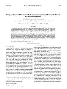
Having an expression for the RWF that combines the effects of pulse compression and range-time signal processing is just the first step. We now need to define constraints on the RWF to meet high-level system requirements. Unfortunately, as mentioned above, typical weather-radar requirements address only one or two aspects of the RWF explicitly. For instance, most requirement documents specify a range resolution, which is typically defined as the 6-dB width of the RWF (Doviak and Zrnic´ 1993), but there are no constraints on the shape of the RWF. However, in the absence of explicit constraints on the RWF, these can be inferred from antenna pattern requirements. If we assume analogous bounding of the radar resolution volume in all polar-coordinate dimensions, then we can extend angular antenna pattern constraints to the range dimension. This can be done by mapping the azimuthal resolution (given by the antenna beamwidth u1) to the range resolution (given by r6). To illustrate how constraints on the RWF can be obtained in practice, let us consider the WSR-88D requirement for the one-way antenna pattern (ROC 2014, p. 3-61): ‘‘In any plane, the first sidelobe shall be less than or equal to 225 dB relative to the peak of the beam. In the region between 628 and 6108, the sidelobe level shall lie below the straight line connecting 225 dB at 628 and 234 dB at 6108. Between 6108 and 61808, the sidelobe envelope shall be less than or equal to 240 dB relative to the peak of the beam.’’ This is shown graphically in Fig. 1, where the two-way maximum angular sidelobe levels corresponding to the one-way specification and a typical WSR-88D two-way antenna radiation pattern are plotted as a function of azimuth angle relative to the center of the beam. An analogous specification can be written for the RWF by mapping the WSR-88D 18 azimuthal beamwidth to the required 250-m range resolution. Although the azimuthal extent of the resolution volume (m) varies with range, this mapping allows the specification of analogous behavior for scatterers outside the required azimuthal and range resolutions (i.e., the impact of scatterers located a given number of azimuthal resolutions away from the center of the radar resolution volume in the azimuth direction is the same as for scatterers located an equal number of range resolutions away in the range direction). However, aside from the 6-dB width (i.e., the antenna pattern is 6 dB below the peak at 6u1/2), the antenna pattern requirement does not specify the complete desired behavior within 62u1 (i.e., no specification is provided for angles within 628 other than the MLW must be 18). This should not be misconstrued as an omission in the WSR88D system specification because the main lobe of typical reflector-antenna patterns (in logarithmic units) can

1356

JOURNAL OF ATMOSPHERIC AND OCEANIC TECHNOLOGY

VOLUME 34

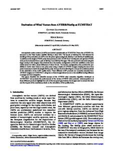
from the sidelobes, which can be a function of the sampling rate. Figure 2 shows the specified range envelope for a required range resolution of 250 m (dotted line) and, as examples, the RWF corresponding to a conventional (rectangular) 1.67-ms CW pulse (black) and a 30-ms NLFM pulse (gray), both with a 250-m range resolution. Mathematically, this range envelope is defined as 8 > : 280 dB r . 2500 m (3)

FIG. 1. Typical WSR-88D two-way antenna radiation pattern as a function of azimuth angle with the specified two-way maximum angular sidelobe levels (dotted lines).

be approximated by a parabola, thus specifying its 6-dB width is enough to fully characterize it. However, the RWF is not guaranteed to have a parabolic main lobe within 62r6 [as illustrated in some of the examples in Torres and Curtis (2012)], so it cannot be fully specified by its 6-dB width. For this purpose, we draw from the performance of a conventional high-power CW pulse with the same required range resolution, which is well understood and accepted. We can now specify constraints on the RWF by defining a range envelope as follows: d

d

For ranges between r6/2 and 2r6 (measured from the center of the resolution volume), the RWF shall not exceed the maximum between 250 dB (i.e., the maximum allowable two-way antenna pattern for the first sidelobe level) and the RWF of a conventional CW pulse with the same range resolution r6. The same applies for ranges between 22r6 and 2r6/2. For ranges larger than 62r6, the RWF shall not exceed the antenna pattern maximum sidelobe levels obtained by mapping the azimuth angle (u) to the range (r) as r 5 ur6 /u1 (i.e., the 6-dB antenna beamwidth maps to the 6-dB range resolution).

Note that no constraints are imposed for ranges within 6r6/2 because the behavior of the RWF in this interval does not generally affect the range resolution. Also, unlike the WRS-88D antenna pattern requirement, the definition for the range envelope does not distinguish between main lobe and sidelobes of the RWF; it simply states that no portion of the RWF shall exceed the range envelope. This is an important simplification, since it saves us from having to distinguish the RWF main lobe

where r is the range from the center of the resolution volume (m), E is the range envelope (dB), and WCW(250) is the RWF of a rectangular CW pulse with a 250-m range resolution (dB).

3. Minimum-bandwidth waveform design Having well-defined RWF requirements described by the range envelope, we now focus on the design of minimum-bandwidth pulse compression waveforms that when combined with range-time processing techniques lead to RWFs that meet range-envelope constraints. We begin by setting up a pulse compression waveform optimization problem and conclude by providing examples for three cases of range-time signal processing. A general base-band pulse compression waveform can be expressed as a function of continuous time t as " e(t) 5 u(t) exp j2p

ðt 22t

# 0

f (t ) dt

0

(4)

for 2t/2 , t , t/2, where t is the pulse width. In this equation, u(t) is the amplitude taper and f(t) is the frequency function such that 2B/2 , f(t) , B/2, where B is the waveform bandwidth. A small amount of amplitude taper helps to reduce sidelobe levels without a significant SNR loss and to avoid sharp amplitude transitions, which are not feasible for a practical implementation. In this case, we adopt the Tukey window (Harris 1978) with parameter 0.1, which results in an SNR loss of 0.24 dB. Note that this amplitude taper is the same as in Kurdzo et al. (2014) and Pang et al. (2015). The frequency function is typically assumed to be odd (leading to good Doppler tolerance and RWF symmetry). Empirical evidence suggests that f(t) should also be strictly monotonic and that its rate of change should be faster at the edges than in the center, since greater chirp rates at the

JUNE 2017

1357

TORRES ET AL.

FIG. 2. RWF using a 1.67-ms rectangular CW pulse (gray) and a 30-ms NLFM pulse (black), both with a 250-m range resolution. The NLFM pulse is tapered in amplitude using a Tukey window with parameter 0.1. This waveform was obtained using the optimization framework described in section 3; it has a bandwidth of 3.14 MHz, and its frequency function is depicted in Fig. 3. The specified range envelope in (3) is shown for a required range resolution of 250 m (dotted lines).

beginning and the end of the pulse produce a similar effect to amplitude tapering with respect to better range sidelobe performance. An example of an NLFM frequency function is shown in Fig. 3 with its corresponding RWF in Fig. 2. In essence, the design of pulse compression waveforms consists of finding the proper frequency function given that the pulse length and amplitude taper are determined by the required sensitivity. The stationary phase principle (Cook and Bernfeld 1993) can be used to determine the phase of a complex modulation signal that results in a predetermined RWF. However, since we are not looking for a predetermined RWF but for one that meets the constraints of the range envelope defined in the previous section, we pose this design problem as an optimization problem. That is, the goal is to find a minimum bandwidth f(t) such that when combined with other range-time signal processing techniques, the resulting RWF meets the constraints of the range envelope illustrated in Fig. 2. For this purpose, the inverse of the frequency function (i.e., time expressed as a function of frequency) is parameterized similarly to Pang et al. (2015) using a generalized series of sinusoids. According to the theory of window design,

this should naturally lead to RWFs with low sidelobes. Mathematically, t tf t t 5 u( f ) 5 1 1 2 B 2p

N

a



å nn2 sin

n51

 2pnf , B

(5)

where N is the number of sinusoids and an (1 # n # N) are real coefficients. Compared to Pang et al.’s approach, our approach is slightly different, as we use a 1/n 2 multiplier instead of 1/n. This modification was added because for well-behaved waveforms, the series coefficients (an/n2) decrease very quickly as n increases. The additional 1/n factor helps ensure a similar order of magnitude for all the an. The RWF can be obtained using (1), where T depends on any additional range-time processing and the modified pulse is obtained as p(lDt) 5 (e*h)(lDt), for 0 # l , Np, where Dt is the range-time sampling period corresponding to Dr and the asterisk (*) denotes convolution. For our purposes, h(t) is the matched compression filter, that is, h(t) 5 e*(2t). As shown in (3), e(t) depends on f(t), which is obtained numerically as the inverse function of u(f) in (5). Because the RWF must meet the constraints of the range envelope, we define a penalty function to quantify

1358

JOURNAL OF ATMOSPHERIC AND OCEANIC TECHNOLOGY

VOLUME 34

FIG. 3. Frequency function corresponding to the RWF of the NLFM pulse in Fig. 2.

how much it exceeds the envelope. The integrated contamination (IC) is defined as ( IC 5 10 log10

1 2NW

) max[W(nDr), E(nDr)] , å E(nDr) n52NW (6)

imposed by the range envelope but without using any additional range-time processing techniques. The constrained optimization problem is defined as

NW

where W is the range weighting function in (1), E is the range envelope in (3), and rmax 5 NWDr is the one-sided support of the RWF. The IC represents the power of the RWF that exceeds the range envelope, averaged over the support of the RWF. Note that an RWF that meets the range-envelope requirement results in IC 5 0 dB [i.e., W(nDr) # E(nDr) for all jnj # NW ]. Figure 4 shows an example of an RWF (solid line) that does not meet the range-envelope requirement (dotted line). Shaded areas (labeled as contamination) depict the power of the RWF that exceeds the range envelope. Next, we provide design examples using the proposed optimization framework and consider three signal processing scenarios: pulse compression without additional range-time signal processing, pulse compression with adaptive pseudowhitening, and pulse compression with incoherent averaging.

a. No additional range-time signal processing In this section we design minimum-bandwidth pulse compression waveforms that meet the requirements

minimize B,

subject to IC 5 0,

(7)

where B is the objective function to be minimized and IC 5 0 is the constraint imposed by the range envelope. This can be converted to an unconstrained optimization

FIG. 4. Example of an RWF (solid line) that does not meet the range-envelope requirement (dotted line). Shaded areas (labeled as contamination) represent the power of the RWF that exceeds the range envelope.

JUNE 2017

TORRES ET AL.

1359

FIG. 5. RWF of waveform A (B 5 2.41 MHz).

problem by turning the constraint into an additive penalty term as minimize (B 1 gIC) ,

(8)

where B 1 gIC is referred to as the fitness function (Deb 2000). Here, g is chosen to be large enough (g 5 20) to keep IC as small as possible (ideally zero). Because of the large search space and the goal of finding the global minimum, we chose the genetic algorithm (Goldberg 1989) solver from MATLAB’s Global Optimization Toolbox. Also, the inverse of the frequency function in (4) is parameterized using N 5 7 sinusoids. The search space for an (n 5 1, . . . , 7) is [21, 1] over a grid of 1001 points. For the bandwidth, the search space is [2, 7] MHz over a grid of 5001 points (i.e., the resolution is 1 kHz). The maximum number of generations is set to 2000, and the other parameters are left at their default values. This setup is used next to design an optimumbandwidth pulse compression waveform. The highlevel system requirements define a 250-m range resolution that is enforced by the range envelope through the penalty term (gIC) in the fitness function. Furthermore, we assume that a pulse width of t 5 50 ms is sufficient to meet the sensitivity requirement. The sampling frequency used in the optimization to generate candidate waveforms is fs 5 30 MHz. The optimum pulse compression waveform produced by this optimization (waveform A) has a B 5 2.41 MHz, and the corresponding RWF is shown in

Fig. 5. Notice that the RWF is within the range envelope, producing an IC of zero. Furthermore, the RWF follows the range envelope closely, which suggests that bandwidth is being used efficiently to meet the design requirements. The inset in the top-left corner shows a zoomed-in version of the main lobe of the RWF. This pulse compression waveform can be used to meet the sensitivity requirement of the radar system while meeting the functional requirements imposed by the range envelope. However, since no additional range-time processing is being applied, the update-time requirement (or alternatively the dataquality requirement) may not be met. In the following subsections, we extend this optimization framework to include other range-time processing techniques. Although sensitivity to Doppler shift (i.e., Doppler tolerance) is not explicitly addressed by the optimization framework, a postanalysis of the RWF confirms that the chosen waveform parameterization, which results in an odd frequency function, leads to acceptable performance for relatively high nonzero Doppler velocities. Figure 6 illustrates this by showing a zoomed-in version of the RWF in Fig. 5 (y 5 0 m s21) and the version corresponding to an extreme Doppler velocity of 50 m s21. It can be seen from this figure that the pulse compression waveform obtained with the proposed optimization framework is tolerant to expected Doppler shifts. That is, the RWF for y 5 50 m s21 shows little distortion: a negligible peak displacement of ;5 m and a ;1-dB exceedance of the range envelope at about 2260 m.

1360

JOURNAL OF ATMOSPHERIC AND OCEANIC TECHNOLOGY

VOLUME 34

FIG. 6. RWF of waveform A (B 5 2.41 MHz) for zero (solid line) and 50 m s21 (dashed line) Doppler velocity targets.

As an interesting exercise, Fig. 7 shows the RWF that results from using the waveform designed assuming no additional range-time processing in conjunction with adaptive pseudowhitening processing. As expected, because the impact of additional range-time processing was not included in the formulation of the optimization problem in (8), the resulting RWFs do not meet the range-envelope constraints: their 6-dB widths are ;272 m for p 5 0 and ;374 m for p 5 1, and the sidelobes for both cases are larger than desired.

b. Adaptive pseudowhitening processing We now explore the design of minimum-bandwidth pulse compression waveforms that when combined with adaptive pseudowhitening processing lead to an RWF that meets range-envelope constraints. In this case, the optimization problem is multiobjective; that is, we would like to minimize the bandwidth and the effect of adaptive pseudowhitening processing at low SNRs, which is quantified by the NEF. The problem can be posed as minimize(B, NEF) subject to IC 5 0.

(9)

A common way to convert a multiobjective optimization problem into a single-objective one is by linearly combining the individual objective functions of the multiobjective optimization problem using positive coefficients (or weights). This method is called the weighted-sum method (Chong and

Zak 2008), and the weights control the relative importance of the individual objective functions. Using the weightedsum method and the penalty-function method described for the previous case, the optimization problem is expressed as minimize(B 1 aNEF 1 gIC) ,

(10)

where a and g are positive real scalars. NEF is the noise gain (dB) computed as 10 log10[tr(TCNTH)/L] (Torres and Zrnic´ 2003), where ‘‘tr’’ denotes the trace of a matrix and the normalized noise correlation matrix CN is explicitly included because the noise after the pulse compression matched filter may not be white. As in the previous setup, g 5 20 ensures a vanishing IC. Notice that a controls the trade-off between bandwidth and noise enhancement. That is, additional bandwidth can be used to design waveforms that lead to less noise enhancement. Through the simultaneous minimization of the bandwidth and the NEF, the waveforms produced are bandwidth optimum for both pulse compression and adaptive pseudowhitening processing. To determine an appropriate value for a, we explored the space of solutions as a was increased from 0.1 to 10 in steps of 0.1. We used the same optimization parameters as in case A with an oversampling factor of L 5 5. Through this process we obtained a locus of optimum solutions delineating a Pareto front (Stadler 1988) that characterizes the tradeoff between B and the NEF as shown in Fig. 8. Notice

JUNE 2017

TORRES ET AL.

1361

FIG. 7. RWF of waveform A (B 5 2.41 MHz) when used in conjunction with adaptive pseudowhitening. Two RWFs correspond to the two extreme cases of adaptive pseudowhitening. PTB with p 5 0 approaches the performance of the matched filter, whereas a PTB with p 5 1 is a whitening transformation.

that the minimum-bandwidth waveform that meets the requirements has a bandwidth of approximately 4.38 MHz (for a 5 0.1) and an NEF of about 1.5 dB. In addition, for a bandwidth greater than approximately 4.7 MHz (with a 5 10), the waveforms have a nearly zero NEF. As an example, we chose a particular optimum waveform from the Pareto front (indicated in Fig. 8 with a black circle) that has a bandwidth of 4.41 MHz and an NEF of 1.2 dB; this waveform is referred to as waveform B. The RWFs corresponding to this waveform and the two extreme cases of adaptive pseudowhitening (i.e., p 5 0 and p 5 1) are shown in Fig. 9. Notice that both ‘‘extreme’’ RWFs meet the rangeenvelope requirement (IC 5 0) and closely follow the range envelope. It can be inferred that the RWFs corresponding to intermediate values of p also meet the range-envelope requirement, since they would lie in between the two extremes. Hence, this optimum pulse compression waveform can be used to simultaneously meet the sensitivity and the update time (or alternatively data quality) requirements of the radar system while meeting the requirements imposed by the range envelope. However, the adaptive pseudowhitening transformation results in larger noise enhancement as the variance reduction increases. In the next subsection we present an optimization

framework that minimizes the waveform bandwidth while considering incoherent-averaging processing to preserve the white noise power at the price of a lower variance reduction.

FIG. 8. NEF vs bandwidth for solutions to the minimumbandwidth optimization problem that considers the use of adaptive pseudowhitening processing for different values of a (0.1, 0.5, 1, 5, and 10). Different marker colors are used to represent sets of solutions for different values of a. Shown is the Pareto front (solid line). Waveform B is on the Pareto front and has a bandwidth of 4.41 MHz and an NEF of 1.2 dB (black circle).

1362

JOURNAL OF ATMOSPHERIC AND OCEANIC TECHNOLOGY

VOLUME 34

FIG. 9. RWF of waveform B (B 5 4.41 MHz) when used in conjunction with adaptive pseudowhitening processing (NEF 5 1.2 dB). Two RWFs correspond to the two extreme cases of adaptive pseudowhitening (PTB with p 5 0 and PTB with p 5 1).

c. Incoherent-averaging processing We now consider the design of minimum-bandwidth pulse compression waveforms that when combined with incoherent-averaging processing lead to RWFs that meet range-envelope constraints. The fitness function in case B is modified to consider the performance of incoherent-averaging processing; that is, instead of minimizing the NEF, which is zero, we would like to maximize the VRF. Since the VRF has an upper bound given by L, maximizing the VRF is equivalent to minimizing (L 2 VRF). Thus, the optimization problem is defined as minimize[B 1 a(L 2 VRF) 1 gIC],

(11)

where, as before, a and g are positive real scalars. VRF is computed as tr(CV)/L2, where CV is the normalized signal correlation matrix (Torres and Zrnic´ 2003). Once again, g 5 20 to ensure a vanishing IC. In this case, a controls the trade-off between bandwidth and VRF; that is, additional bandwidth can be used to design waveforms that lead to higher variance reduction. This optimization framework produces pulse compression waveforms with minimum bandwidth that lead to maximum VRF when combined with incoherent averaging. As before, we explored the space

of solutions as a was increased from 0.1 to 10 in steps of 0.1 using the same optimization parameters as in case A and an oversampling factor of L 5 5. We obtained a set of optimum solutions delineating a Pareto front that characterizes the trade-off between B and VRF as shown in Fig. 10. Notice that the minimum-bandwidth waveform that meets the requirements (for a 5 0.1) has a bandwidth of approximately 4.32 MHz and a VRF of about 3.4. Furthermore, as in case A, for a bandwidth greater than approximately 4.7 MHz, we can obtain waveforms for which the VRF is approximately L. In this example we chose a particular optimum waveform from the Pareto front (indicated in Fig. 10 with a black circle) that has a bandwidth of 4.41 MHz (similar to case B) and a VRF of 3.85; this waveform is referred to as waveform C. The RWF corresponding to this waveform is shown in Fig. 11. As before, this solution meets the range-envelope requirement (IC 5 0) and closely follows the range envelope. Similar to the solution presented in case B, this optimum pulse compression waveform can simultaneously meet the sensitivity and the update-time (or alternatively data quality) requirements of the radar system while meeting the requirements imposed by the range envelope. However, incoherent-averaging processing may not achieve the full variance reduction of L.

JUNE 2017

TORRES ET AL.

1363

FIG. 10. VRF for reflectivity estimates vs bandwidth for solutions to the minimum-bandwidth optimization problem that considers the use of incoherent averaging for different values of a (0.1, 0.5, 1, 5, and 10). Different marker colors are used to represent sets of solutions for different values of a. Shown is the Pareto front (solid line). Waveform C is on the Pareto front and has a bandwidth of 4.41 MHz and a VRF of 3.85 (black circle).

d. Discussion Cases A–C presented waveforms that meet the system requirements defined in this paper when coupled with different range-time processing techniques. Improved data-quality performance through additional range-time processing results in waveforms with larger bandwidth (cf. 2.41 MHz for waveform A with 4.41 MHz for waveforms B and C). However, with adaptive pseudowhitening processing, the variance of estimates can be reduced by a factor of L at high SNRs. This improvement comes at a price of increased noise gain, which is more evident at low SNRs. Using incoherent averaging involves computationally simpler processing, but the variance of estimates can be reduced by a factor smaller than L. Figure 12 shows a comparison of the VRFs as a function of the SNR obtained with waveforms A–C when coupled with different types of range-time processing. In all cases, the VRF is computed with respect to using waveform A with no additional range-time processing. We had previously shown that using the low-bandwidth waveform A with adaptive pseudowhitening processing led to an RWF that did not meet the range-envelope requirements. Additionally, Fig. 12 shows that this mismatched combination of waveform and range-time processing leads to reduced performance in

terms of VRF, especially at low-to-medium SNRs. At high SNRs, adaptive pseudowhitening processing leads to a maximum VRF of 5, but the performance at low-tomedium SNRs is better for waveform B than it is for waveform A. This makes sense, since waveform B was optimized, taking into account the use of adaptive pseudowhitening processing. Furthermore, the combination of waveform C and incoherent-averaging processing results in reduced performance compared to waveform B with adaptive pseudowhitening processing, with VRF values reaching only 3.85 at medium-to-high SNRs. Note that the relative performance holds only for these particular waveforms. If a bandwidth of around 4.8 MHz was used for the waveforms designed for range-time signal processing, then the performance of an appropriately optimized adaptive pseudowhitening waveform and an appropriately optimized incoherent-averaging waveform would perform similarly with both low noise gain and VRFs near L. In the next section, we use simulations to qualitatively compare the performance of the three designed waveforms.

4. Weather data simulations In this section we compare the performance of the three waveforms from section 3 using a simulator based

1364

JOURNAL OF ATMOSPHERIC AND OCEANIC TECHNOLOGY

VOLUME 34

FIG. 11. RWF of waveform C (B 5 4.41 MHz) when used in conjunction with IAB (VRF 5 3.85).

on real weather data fields. This also gives us the flexibility to compare the designed waveforms to a conventional high-powered pulse—a comparison that would not be possible on most radar systems. The weather simulator utilizes WSR-88D radar-variable data available from the National Centers for Environmental Information (NCEI) to produce simulated data with particular signal characteristics. This approach allows us to choose different values for the number of samples per dwell M and different PRTs. However, because of certain issues with the NCEI data, several processing steps are needed before inphase and quadrature-phase (IQ) time series can be simulated. These processing steps and the time series simulation steps are briefly described next. After data for all six radar variables (three spectral moments and three dual-polarization variables) are retrieved for a complete constant-elevation scan, the reflectivity is converted back to signal power. The data are then spatially smoothed to remove some of the measurement variability and also to fill in values that were censored in the original processing. On the WSR88D, a lower SNR threshold is typically used to censor reflectivity data (compared to the threshold used for other variables); thus, we need to produce reasonable values for those variables where data do not exist, since all six variables are needed to simulate dual-polarization time series. A robust smoother was chosen to fill in

missing values and to extend the radar-variable fields when necessary. The algorithm works by iteratively applying a low-pass filter in the discrete cosine transform domain until the power-normalized spatial variance of the difference between the filtered and measured fields is minimized (Garcia 2010). The smoothed reflectivity field is used to determine where weather signals are simulated; areas without weather signals have only simulated noise. After the radar-variable data are conditioned, the variables are resampled (using interpolation) on the chosen azimuth-by-range grid. The range spacing needs to be sufficiently small to match the bandwidth of the waveforms used for pulse compression, so 25-m range spacing (corresponding to 6 MHz sampling) is utilized. To impose the proper range correlation on the data corresponding to each waveform, a scattering-center simulation approach is used. This type of simulation is commonly employed when simulating range-oversampled data (e.g., Curtis and Torres 2013). Independent sequences of M dual-polarization time series samples are simulated for each scattering center along range using the six radar variables sampled for that range and azimuth location. The range correlation is then imposed by convolving the time series data in range with the waveform (sampled at 6 MHz). This closely represents the time series as it would appear at the output of the radar receiver and before processing.

JUNE 2017

TORRES ET AL.

1365

FIG. 12. VRF for reflectivity estimates as a function of the SNR for the waveforms and processing scenarios of Fig. 5 (waveform A with no additional range-time processing, dotted gray line), Fig. 7 (waveform A with adaptive pseudowhitening processing, dotted black line), Fig. 9 (waveform B with adaptive pseudowhitening processing, solid black line), and Fig. 11 (waveform C with incoherent averaging processing, solid gray line).

The final step after simulating the time series is to process each set appropriately for each waveform. The data corresponding to the pulse compression waveform with no additional signal processing (case A) has only the pulse compression matched filter applied; these data are then decimated to produce data with 250-m range spacing to correspond to the other cases. The adaptive pseudowhitening waveform data (case B) are also processed with the corresponding matched filter. The data are then decimated to produce data with 50-m range spacing so that additional range-time signal processing can be performed. The adaptive pseudowhitening processing is applied along range to sets of L 5 5 consecutive range bins, resulting in 250-m data after processing. The data corresponding to the third waveform with incoherent averaging (case C) is also processed with the appropriate pulse compression matched filter and decimated to 50 m. The correlations needed to compute the radar variables are then incoherently averaged along range, again in sets of five, before computing the radar variables. This results in data with 250-m range spacing that match the other cases. The fourth and fifth cases were simulated using a conventional CW pulse with the same average power as the pulse

compression waveforms. One case involves no additional range-time signal processing and the other one uses adaptive pseudowhitening processing. These cases illustrate the performance of a high-power conventional waveform and allow for the comparison with the performance of the pulse compression waveforms. The conventional-waveform data are simulated with 25-m range spacing and are decimated to 50-m range spacing after an antialiasing filter is applied.2 For the conventional adaptive pseudowhitening case, the same adaptive pseudowhitening processing is used as in case B with the appropriate range-correlation matrix. As an example, data collected at 1100 UTC 6 June 2014 with the KTLX radar (Oklahoma City, Oklahoma) were retrieved from the NCEI website. The data were collected using volume coverage pattern (VCP) 212 with systematic phase code (SZ-2) processing (Torres 2005). Data collected with SZ-2 processing are preferred for these simulations because there are less range-overlaid Doppler

2

Note that the antialiasing filter is not necessary in the pulse compression cases because the pulse compression matched filter already sufficiently reduces the bandwidth.

1366

JOURNAL OF ATMOSPHERIC AND OCEANIC TECHNOLOGY

velocity and spectrum width data (or ‘‘purple haze’’) compared to data processed using legacy range-unfolding algorithms. The simulated data utilized a PRT of 3 ms and 16 samples and were simulated with 25-m range bins as mentioned previously. Figure 13 shows portions of five plan position indicators (PPIs) corresponding to the five cases described above. There are no obvious differences in range resolution or evidence of range-sidelobe contamination in any of the PPIs, which is consistent with the range-envelope requirement. Both the conventional pulse and the pulse compression waveform without additional range-time processing clearly have the highest variance of reflectivity estimates. The range-time processing for the other three cases significantly reduces the variance, resulting in smoother fields. The pulse compression waveforms with and without adaptive pseudowhitening processing perform comparably to the conventional pulse with the same processing except for a slight decrease in sensitivity. Incoherent averaging also appears to reduce the variance well, but there is an additional small loss in sensitivity compared to the adaptive pseudowhitening cases. The minor differences in sensitivity can be explained by small differences in the widths of the compressed pulses, which lead to slightly different matched-filter bandwidths. Overall, the simulations reflect the design parameters used to produce the waveforms. The predicted difference in VRF between incoherent averaging and adaptive pseudowhitening can be difficult to discern in a PPI image. Figure 14 uses a measurement of spatial variability to estimate the VRF from the data. The true power (known because the data are simulated) was used to scale the simulated powers, which normalizes the spatial variance. A smoothing filter was applied after calculating the spatial variance (using a running 11 3 11 window), and point-by-point ratios were computed to produce the final result. The VRF for adaptive pseudowhitening is uniformly larger than the VRF for incoherent averaging, which is consistent with the theoretical VRFs computed in Fig. 12. These plots may not be quite as smooth as expected, but the spatial variability only partially reflects the true VRF. At a bandwidth of around 4.4 MHz, both the adaptive pseudowhitening and incoherentaveraging waveforms perform as designed with the adaptive pseudowhitening waveform producing reflectivity data with more variance reduction at high SNRs.

5. Conclusions In this paper we proposed a requirement-driven approach for the design of pulse compression waveforms for weather radars. Because explicit requirements on the range weighting function (RWF) are typically not provided, the criteria used for the antenna-sidelobe

VOLUME 34

envelope on the WSR-88D were extended to derive an analogous range envelope for the RWF. Whereas WSR88D requirements were used in this work, the proposed approach can be adapted to any low-power weatherradar system that employs pulse compression; that is, the same methodology can be used to derive a systemspecific range envelope based on particular system requirements. Additionally, we proposed an optimization framework that produces minimum-bandwidth pulse compression waveforms that meet high-level system requirements. This proposed framework considers the impact on the RWF of the transmitted waveform and also of any range-time signal processing technique that may be needed to meet data-quality and/or update-time requirements. To demonstrate the generality of the proposed approach, fitness functions were tailored for three processing scenarios: pulse compression without additional range-time processing, pulse compression with adaptive pseudowhitening processing, and pulse compression with incoherent-averaging processing. The performance of these waveforms was illustrated using simulations based on real weather data fields, and the results were compared to the performance of conventional high-power transmitter systems. Although some practical effects like amplitude droop and phase distortions were ignored in this analysis, the proposed optimization framework can be easily extended to include predistortion and/or other compensation schemes. Despite the idealized configuration, the results of this work indicate that it is possible to design weather-radar pulse compression waveforms that when combined with other range-time signal processing techniques meet high-level system requirements. By deriving explicit pulse compression requirements for weather radars, it is possible to use a requirement-driven waveform design approach. Such an approach ensures that pulse compression waveforms meet relevant requirements with minimum cost in terms of transmission bandwidth and signal processing complexity. These design criteria are explicit in the proposed optimization framework, where a tailored fitness function was provided that favors waveforms with smaller transmission bandwidths while penalizing those RWFs that exceed the required range envelope. In partnership with the Federal Aviation Administration (FAA), NOAA is currently developing the Advanced Technology Demonstrator (ATD), a midscale, dual-polarized multifunction phased-array radar at the National Weather Radar Testbed in Norman, Oklahoma. This radar will combine the use of pulse compression (to meet sensitivity and range-resolution requirements) with range-time signal processing techniques (to meet data-quality and/or update-time

JUNE 2017

TORRES ET AL.

FIG. 13. Zoomed-in reflectivity fields with (top left) a 1.67-ms high-power CW pulse with no additional range-time processing (HP CW), (top right) a 1.67-ms high-power CW pulse using adaptive pseudowhitening range-time processing (HP CW 1 APTB), (middle left) waveform A with no additional range-time processing (PC), (middle right) waveform B with adaptive pseudowhitening range-time processing (PC 1 APTB), and (bottom right) waveform C with incoherent-averaging range-time processing (PC 1 IAB).

1367

1368

JOURNAL OF ATMOSPHERIC AND OCEANIC TECHNOLOGY

VOLUME 34

FIG. 14. Zoomed-in estimated variance-reduction-factor fields for the same region shown in Fig. 13. (left) Ratio of variances of reflectivity estimates using a pulse compression waveform with adaptive pseudowhitening processing (PC 1 APTB) relative to using pulse compression with no additional range-time processing (PC). (right) As in the left panel, but comparing pulse compression and incoherentaveraging processing (PC 1 IAB) to PC.

requirements). Thus, the ATD will be an ideal platform to test the pulse compression waveforms designed with the proposed framework. In general, the requirements derived herein should provide a solid foundation to facilitate the design of other modern weather-radar systems based on solid-state transmitters with expected performance similar to that of traditional systems based on high-power transmitters. Acknowledgments. Funding was provided by NOAA/ Office of Oceanic and Atmospheric Research under NOAA–University of Oklahoma Cooperative Agreement NA11OAR4320072, U.S. Department of Commerce. REFERENCES Ashe, J. M., R. L. Nevin, D. J. Murrow, H. Urkowitz, N. J. Bucci, and J. D. Nespor, 1994: Range sidelobe suppression of expanded/ compressed pulses with droop. 1994 IEEE Radar Conference, IEEE, 116–122, doi:10.1109/NRC.1994.328109. Austin, G. L., 1974: Pulse compression systems for use with meteorological radars. Radio Sci., 9, 29–33, doi:10.1029/ RS009i001p00029. Bharadwaj, N., and V. Chandrasekar, 2012: Wideband waveform design principles for solid-state weather radars. J. Atmos. Oceanic Technol., 29, 14–31, doi:10.1175/JTECH-D-11-00030.1. Brown, R. A., V. T. Wood, and R. M. Steadham, 2001: Faster and denser scanning strategies for WSR-88Ds. Preprints, 26th

National Weather Association Annual Meeting, Spokane, WA, National Weather Association, 31–32. ——, ——, and D. Sirmans, 2002: Improved tornado detection using simulated and actual WSR-88D data with enhanced resolution. J. Atmos. Oceanic Technol., 19, 1759–1771, doi:10.1175/1520-0426(2002)019,1759:ITDUSA.2.0.CO;2. Bucci, N. J., H. S. Owen, K. A. Woodward, and C. M. Hawes, 1997: Validation of pulse compression techniques for meteorological functions. IEEE Geosci. Remote Sens. Lett., 35, 507–523, doi:10.1109/36.581958. Cheong, B. L., R. Kelley, R. D. Palmer, Y. Zhang, M. Yeary, and T.-Y. Yu, 2013a: PX-1000: A solid-state polarimetric X-band weather radar and time–frequency multiplexed waveform for blind range mitigation. IEEE Trans. Instrum. Meas., 62, 3064– 3072, doi:10.1109/TIM.2013.2270046. ——, J. M. Kurdzo, G. Zhang, and R. D. Palmer, 2013b: The impacts of multi-lag moment processor on a solid-state polarimetric weather radar. 36th Conf. on Radar Meteorology, Breckenridge, CO, Amer. Meteor. Soc., 2B.2. [Available online at https://ams.confex.com/ams/36Radar/webprogram/ Paper228464.html.] Chong, E., and S. Zak, 2008: An Introduction to Optimization. Wiley, 584 pp. Cook, F., and M. Bernfeld, 1993: Radar Signals. Artech House, 532 pp. Curtis, C., and S. Torres, 2011: Adaptive range oversampling to achieve faster scanning on the National Weather Radar Testbed phased-array radar. J. Atmos. Oceanic Technol., 28, 1581–1597, doi:10.1175/JTECH-D-10-05042.1. ——, and ——, 2013: Real-time measurement of the range correlation for range oversampling processing. J. Atmos. Oceanic Technol., 30, 2885–2895, doi:10.1175/JTECH-D-13-00090.1.

JUNE 2017

TORRES ET AL.

Deb, K., 2000: An efficient constraint handling method for genetic algorithms. Comput. Methods Appl. Mech. Eng., 186, 311–338, doi:10.1016/S0045-7825(99)00389-8. Doviak, R., and D. Zrnic´, 1993: Doppler Radar and Weather Observations. 2nd ed. Academic Press, 562 pp. Ducoff, M., and B. Tietjen, 2008: Pulse compression radar. Radar Handbook, 3rd ed. M. I. Skolnik, Ed., McGraw-Hill, 8.1–8.44. Efremov, V., I. Vylegzhanin, and B. Vovshin, 2011: The new generation of Russian C-band meteorological radars. Technical features, operation modes and algorithms, Proceedings of the 12th International Radar Symposium (IRS 2011), H. Rohling, Ed., IEEE, 239–244. Fetter, R. W., 1970: Radar weather performance enhanced by compression. Preprints, 14th Conf. in Radar Meteorology, Tucson, AZ, Amer. Meteor. Soc., 413–418. Garcia, D., 2010: Robust smoothing of gridded data in one and higher dimensions with missing values. Comput. Stat. Data Anal., 54, 1167–1178, doi:10.1016/j.csda.2009.09.020. Goldberg, D. E., 1989: Genetic Algorithms in Search, Optimization and Machine Learning. Addison-Wesley, 432 pp. Griffiths, H., and L. Vinagre, 1994: Design of low-sidelobe pulse compression waveforms. Electron. Lett., 30, 1004–1005, doi:10.1049/el:19940644. Harris, F. J., 1978: On the use of windows for harmonic analysis with the discrete Fourier transform. Proc. IEEE, 66, 51–83, doi:10.1109/PROC.1978.10837. Heinselman, P. L., D. L. Priegnitz, K. L. Manross, T. M. Smith, and R. W. Adams, 2008: Rapid sampling of severe storms by the National Weather Radar Testbed Phased Array Radar. Wea. Forecasting, 23, 808–824, doi:10.1175/2008WAF2007071.1. Kurdzo, J. M., B. L. Cheong, R. D. Palmer, G. Zhang, and J. B. Meier, 2014: A pulse compression waveform for improvedsensitivity weather radar observations. J. Atmos. Oceanic Technol., 31, 2713–2731, doi:10.1175/JTECH-D-13-00021.1. Middleton, C. A., and J. Given, 2011: The next broadband challenge: Wireless. J. Inf. Policy, 1, 36–56, doi:10.5325/ jinfopoli.1.2011.0036. Mudukutore, A. S., V. Chandrasekar, and R. J. Keeler, 1998: Pulse compression for weather radars. IEEE Trans. Geosci. Remote Sens., 36, 125–142, doi:10.1109/36.655323. Mueller, E. A., 1977: Statistics of high radar reflectivity gradients. J. Appl. Meteor., 16, 511–513, doi:10.1175/1520-0450(1977)016,0511: SOHRRG.2.0.CO;2. Nakagawa, K., H. Hanado, N. Takahashi, S. Satoh, K. Fukutani, and T. Iguchi, 2006: Development of a C-band polarimetric and pulse compression radar in Okinawa, Japan. 2006 IEEE International Symposium on Geoscience and Remote Sensing, IEEE, 1670–1673, doi:10.1109/IGARSS.2006.431. Nguyen, C. M., and V. Chandrasekar, 2014: Sensitivity enhancement system for pulse compression weather radar. J. Atmos. Oceanic Technol., 31, 2732–2748, doi:10.1175/ JTECH-D-14-00049.1. NOAA/NWS, 2015: Radar functional requirements. NOAA/NWS Internal Rep., 58 pp.

1369

O’Hora, F., and J. Bech, 2007: Improving weather radar observations using pulse-compression techniques. Meteor. Appl., 14, 389–401, doi:10.1002/met.38. Pang, C., P. Hoogeboom, F. Le Chevalier, H. W. J. Russchenberg, J. Dong, T. Wang, and X. Wang, 2015: A pulse compression waveform for weather radars with solid-state transmitters. IEEE Geosci. Remote Sens. Lett., 12, 2026–2030, doi:10.1109/ LGRS.2015.2443551. ROC, 2014: WSR-88D system specification. NOAA Doc. 2810000J, 174 pp. [Available from WSR-88D Radar Operations Center (ROC), 1313 Halley Circle, Norman, OK 73069.] Rockwell, M., 2017: FAA looks to spur spectrum sharing tech. [Available online at https://fcw.com/articles/2017/01/06/faaspectrum-sensr.aspx.] Rogers, R., 1971: The effect of variable target reflectivity on weather radar measurements. Quart. J. Roy. Meteor. Soc., 97, 154–167, doi:10.1002/qj.49709741203. Sanders, F., R. Sole, B. Bedford, D. Franc, and T. Pawlowitz, 2006: Effects of RF interference on radar receivers. NTIA Tech. Rep. TR-06-444, 162 pp. [Available online at http://www.its. bldrdoc.gov/publications/2481.aspx.] ——, ——, J. Carroll, G. Secrest, and T. Allmon, 2012: Analysis and resolution of RF interference to radars operating in the band 2700-2900 MHz from broadband communication transmitters. NTIA Tech. Rep. TR-13-490, 147 pp. [Available online at http://www.its.bldrdoc.gov/publications/2684.aspx.] Stadler, W., 1988: Multicriteria Optimization in Engineering and in the Sciences. Plenum Press, 406 pp. Stailey, J., 2017: Spectrum Efficient National Surveillance Radar (SENSR): Overview of the ‘‘new MPAR.’’ 33rd Conf. on Environmental Information Processing Technologies, Seattle, WA, Amer. Meteor. Soc., 6.1. [Available online at https://ams. confex.com/ams/97Annual/webprogram/Paper303355.html.] Torres, S., 2005: Range and velocity ambiguity mitigation on the WSR-88D: Performance of the SZ-2 phase coding algorithm. Preprints, 21st Int. Conf. on Interactive Information and Processing Systems (IIPS) for Meteorology, Oceanography, and Hydrology, San Diego, CA, Amer. Meteor. Soc., 19.2. [Available online at https://ams.confex.com/ams/Annual2005/ techprogram/paper_83946.htm.] ——, and D. Zrnic´, 2003: Whitening in range to improve weather radar spectral moment estimates. Part I: Formulation and simulation. J. Atmos. Oceanic Technol., 20, 1433–1448, doi:10.1175/1520-0426(2003)020,1433:WIRTIW.2.0.CO;2. ——, and C. D. Curtis, 2012: The impact of signal processing on the range-weighting function for weather radars. J. Atmos. Oceanic Technol., 29, 796–806, doi:10.1175/JTECH-D-11-00135.1. Urkowitz, H., and S. Katz, 1996: The relation between range sampling rate, system bandwidth, and variance reduction in spectral averaging for meteorological radar. IEEE Trans. Geosci. Remote Sens., 34, 612–618, doi:10.1109/36.499741. Zrnic´, D. S., and R. J. Doviak, 2005: System requirements for phased array weather radar. NOAA/NSSL Rep., 23 pp. [Available online at http://www.nssl.noaa.gov/publications/ mpar_reports/LMCO_Consult2.pdf.]