Research Article Dynamic Neural Network Identification and

Hindawi Publishing Corporation Abstract and Applied Analysis Volume 2014, Article ID 316206, 10 pages http://dx.doi.org/10.1155/2014/316206

Research Article Dynamic Neural Network Identification and Decoupling Control Approach for MIMO Time-Varying Nonlinear Systems Zhixi Shen and Kai Zhao School of Automation, Chongqing University, Chongqing 400044, China Correspondence should be addressed to Zhixi Shen; [email protected] Received 12 December 2013; Accepted 7 January 2014; Published 13 March 2014 Academic Editor: Xiaojie Su Copyright © 2014 Z. Shen and K. Zhao. This is an open access article distributed under the Creative Commons Attribution License, which permits unrestricted use, distribution, and reproduction in any medium, provided the original work is properly cited. Overcoming the coupling among variables is greatly necessary to obtain accurate, rapid and independent control of the real nonlinear systems. In this paper, the main methodology, on which the method is based, is dynamic neural networks (DNN) and adaptive control with the Lyapunov methodology for the time-varying, coupling, uncertain, and nonlinear system. Under the framework, the DNN is developed to accommodate the identification, and the weights of DNN are iteratively and adaptively updated through the identification errors. Based on the neural network identifier, the adaptive controller of complex system is designed in the latter. To guarantee the precision and generality of decoupling tracking performance, Lyapunov stability theory is applied to prove the error between the reference inputs and the outputs of unknown nonlinear system which is uniformly ultimately bounded (UUB). The simulation results verify that the proposed identification and control strategy can achieve favorable control performance.

1. Introduction Coupling is a widespread phenomenon existing in nonlinear systems. Due to the existence of the coupling, the variables among systems often suffer impact from each other’s fluctuations. Besides, time-varying and time delay is frequently encountered in many real control systems, and these may be the root of instability in the performance of closedloop system. If the problems which have attracted many researchers cannot be solved effectively, they would not only delay achieving the steady states, but also realize the goal of independent control at all. Thereby, in order to achieve accurate, rapid, and independent control, it is essential to decouple among these variables and take the related methods. However, how to select the proper methodology according to the characteristics of control object is a thorny question. In the open pieces of literature, the traditional decoupling ways to a multi-input multioutput (MIMO) system are primarily represented by frequency domain methods such as state variable method, diagonal dominance matrix, characteristic curve method, inverse Nyquist array, and relative gain analysis method [1]. These methods, which are based

on rigorous transfer functions or state spaces, play a significant role in decoupling the linear time-invariant systems. Nevertheless, these methods are hard to accomplish dynamic decoupling for uncertain, nonlinear, and time-variant MIMO systems because precise system models are difficult to develop for these systems. Hence, the above traditional decoupling methods are limited to a certain extent. With the development of decoupling control, many other decoupling approaches, such as adaptive decoupling [2, 3], energy decoupling [4, 5], disturbance decoupling [6, 7], robust decoupling [8, 9], prediction decoupling, intelligent decoupling methods mainly represented by fuzzy decoupling [10], and neural network (NN) decoupling [11], have been proposed and applied in many real control practices. Adaptive decoupling has merits in decoupling a system with uncertain factors and can solve the system’s uncertainty to some extent. However, the algorithm of adaptive controller has a large amount of calculation and is much time consumed [12] so that it is hard to be implemented in the processing of real-time control. Energy decoupling can be applied in linear uncertain systems, but, up to now, the method is also confined to the research stage [13]. Disturbance decoupling

2 [14, 15] tries to perfectly eliminate the external influences on system outputs, but the feasibility of this method has closer relationship with the development of nonlinear system differential geometry theory which is too strict and complex, so some researchers think this approach is very trouble to be widely used in the real control processes. Robust decoupling attempts to design a compensator with both good dynamic performance and strong robustness, but it is tough to deal well with the inner contradiction between the dynamic performance and the optimal decoupling controller parameters of robustness. Intelligent decoupling methods have obvious advantages in decoupling nonlinear systems and have received a lot of interest in decoupling control fields. The representative of intelligent decoupling methods, NN decoupling, has self-learning, adaptive, and fault tolerance abilities and is an universal approximator which has the capability of approximating any nonlinear function to any desired degree of accuracy, making it a useful tool for decoupling control in MIMO nonlinear systems. But NN decoupling commonly requires to be combined with other related algorithms to realize decoupling control [11, 16]. Fuzzy decoupling accomplishes the system decoupling by defuzzification based on the fuzzy rules which are often summarized by practical experiences. For the simple systems, it can be achieved easily, but for more complex MIMO nonlinear systems the accurate multidimensional fuzzy rules are very difficult, even impossible, to be established [17]. In practice, allowing for a complicated MIMO nonlinear system with uncertainty and strong coupling, the common PID controller with fixed parameters can hardly achieve the desired steady sate at all. At the same time, the physical system is often difficult to obtain accurate and faithful mathematical model so that the conventional control schemes based on precise mathematical model can hardly achieve good performance in the real control process. Motivated by the seminal paper [18], there is a continuously increasing interest in applying neural network to identification and control of nonlinear system. In structure, neural networks can be classified as dynamic and feedforward ones. However, most of practical applications use the feedforward structures [19, 20], which are suitable for the approximation of complex static functions. Nevertheless, the major shortcomings of such structure of neural networks in describing dynamic functions are that the weight updating does not utilize the information on the local date structure and the function approximation is sensitive to the purity of training data. On the other hand, the dynamic neural networks [21–24] incorporate feedback not merely having concise structure but more importantly having adaptive mechanism incorporated to fine tune the approximation accuracy and convergent speed. So dynamic neural network (DNN) is being developed, which is superior to the static neural network such as radial basis function (RBF) and backpropagation (BP) neural network on the dynamic characteristic [25, 26] recent years, and it is now widely applied in the fields of system identification and MIMO nonlinear control. In this paper, we focus on developing an indirect adaptive NN controller for complex nonlinear systems including strong coupling, unknown or uncertain models, and

Abstract and Applied Analysis disturbances simultaneously. The proposed method is the combination of NN-based identifier and adaptive controller, and the controller is designed based on the identified NN model. The main merits of this paper can be summarized as follows. (1) A novel and generalized decoupling control strategy based on indirect adaptive control is presented for nonlinear systems. Firstly, we construct a dynamic neural network (DNN) identifier without coupling to replace the real coupled systems. Then, we design the adaptive controller to deal with the nonlinear systems based on DNN identifier models. (2) According to the Lyapunov methodology, the online weights updating laws of DNN are developed to accommodate the identification and to guarantee that the error between the DNN identifier and the real unknown systems is UUB. (3) According to the Lyapunov methodology, the adaptive control laws are designed to deal with modeling uncertainties, system nonlinearities, and external disturbances and to guarantee stable tracking performance of the real outputs related to the reference inputs. This paper is structured in the following way. In Section 2, the problem formulation and preliminaries are presented, in which a general nonlinear dynamic system model and its neural network approximator are presented to establish a basis for designing and analyzing the system identification and control. In Section 3, a DNN-based identification algorithm is developed to approximate the nonlinear system. Section 4 proposed the adaptive decoupling control algorithm based on the DNN identifier. In Section 5, the whole procedure for the identification and control is described to provide a step by step guide for potential users. The simulation results demonstrate the effectiveness and generality of the proposed algorithm in Section 6. Finally, in Section 7 the conclusion is summarized.

2. Problem Formulation and Preliminaries The equation of MIMO continuous-time-varying nonlinear coupling system can be generally described as 𝑦 = 𝑔 (𝑥, 𝑢, 𝑡) ,

(1)

where 𝑥 = [𝑥1 , 𝑥2 , . . . , 𝑥𝑛 ]𝑇 is the state vector of nonlinear system, 𝑢 = [𝑢1 , 𝑢2 , . . . , 𝑢𝑛 ]𝑇 is the bounded control input vector, 𝑦 = [𝑦1 , 𝑦2 , . . . , 𝑦𝑛 ]𝑇 is the output vector, and 𝑔(⋅) is an unknown continuous nonlinear smooth function. In this study, the following assumptions are imposed. Assumption 1. The whole system can be decomposed as 𝑁 coupling subsystems. The architecture of the multi-input multioutput nonlinear system is shown in Figure 1. Assumption 2. All the states of system are bounded and measurable at every instant. The desired output trajectory and its first derivative are bounded.

Abstract and Applied Analysis y1

u1

u1

y2

u2

.. .

3

Plant

.. .

f(xnnn )

y1 Plant 1

f(xnn1 )

.. .

.. .

u1 u2

un

yn un

. ..

Plant N

u=

yn

.. .

b1n .. . b11

f f

∫

∑

u1 .. .

xnn1

− a1 .. .

un

un

bnn .. . bn1

Figure 1: The architecture of the MIMO nonlinear system.

∑

∫

xnn

− f(xnn )

an

DNN-based idientifier

xnn

Figure 3: The architecture of DNN-based identifier. E

u Plant

We consider a single-layer, fully interconnected DNN as follows [25, 27]:

x

Figure 2: The architecture of system identification based on DNN.

In order to analyze the dynamic characteristic of nonlinear system more conveniently, we use the state-space equation to describe system (1) as follows: 𝑥1̇ = 𝑔1 (𝑥, 𝑢1 , 𝑢2 , . . . , 𝑢𝑛 ) 𝑥2̇ = 𝑔2 (𝑥, 𝑢1 , 𝑢2 , . . . , 𝑢𝑛 ) .. . 𝑥𝑛̇ = 𝑔𝑛 (𝑥, 𝑢1 , 𝑢2 , . . . , 𝑢𝑛 ) 𝑦1 = 𝑥1

(2)

𝑦2 = 𝑥2 .. . 𝑦𝑛 = 𝑥𝑛 . By qualitatively analyzing the above model (2), it can be seen that the system is a coupling, time-varying, and uncertain nonlinear system. It is difficult, even impossible, to establish the accurate mathematical model and achieve prefect performance by using traditional decoupling control methods. In this paper, the dynamic neural network 𝑔𝑛𝑛 (𝑥𝑛𝑛 ) will be employed to approximate the continuous nonlinear function 𝑔(𝑥), so that 𝑔 (𝑥) = 𝑔𝑛𝑛 (𝑥𝑛𝑛 ) .

(3)

To identify the coupling, uncertain, and nonlinear dynamic system (2), we use dynamic neural network as the identifier and construct the identification structure as shown in Figure 2.

̇ = 𝐴𝑥𝑛𝑛 + 𝐵𝑓 (𝑥𝑛𝑛 ) + 𝑢, 𝑔𝑛𝑛 (𝑥𝑛𝑛 ) = 𝑥𝑛𝑛

(4)

𝑛

where 𝑥𝑛𝑛 ∈ R is the state variables of DNN, 𝐴 = diag[−𝑎1 , . . . , −𝑎𝑛 ] ∈ R𝑛×𝑛 , 𝑎𝑖 > 0, 𝑖 = 1, . . . , 𝑛 is the unknown matrix for the linear part of NN model, 𝐵 ∈ R𝑛×𝑛 is the matrix of synaptic weights for nonlinear system feedback, 𝑓(𝑥𝑛𝑛 ) = [𝑓(𝑥𝑛𝑛1 ), . . . , 𝑓(𝑥𝑛𝑛𝑛 )]𝑇 is the vector of network feedback, 𝑓(⋅) represents the neuron activation function, and 𝑢 = [𝑢1 , . . . , 𝑢𝑛 ]𝑇 is the control force vector of adaptive controller, which will be designed subsequently. In this work, the architecture of DNN-based identifier is shown in Figure 3. Remark 1. The real system is a coupling, time-varying, and uncertain nonlinear system. Since neural network is a universal approximator which is capable of approximating any nonlinear function to any desired degree of accuracy, we can use DNN model without coupling to replace the real coupled system. This idea motivates a novel and generalized decoupling control strategy based on indirect adaptive control as described in what follows. Using this basic idea, the specific design for DNN-based identifier can be developed in the next section.

3. System Identification Based on Neural Networks The nonlinear system (2) can be approximated by the following continuous dynamic neural networks: 𝑥̇ = 𝐴∗ 𝑥 + 𝐵∗ 𝑓 (𝑥) + 𝑢,

(5)

where 𝐴∗ and 𝐵∗ are ideal nominal constant matrices and the state and output variables are physically bounded. In the process of approximating the time-varying, coupling, nonlinear system, DNN model (4) can be rewritten as follows: ̂ 𝑛𝑛 + 𝐵𝑓 ̂ (𝑥𝑛𝑛 ) + 𝑢, ̇ = 𝐴𝑥 𝑥𝑛𝑛

(6)

4

Abstract and Applied Analysis

where the activation function is specified as a monotonically increased function and bounded with 0 ≤ 𝑓 (𝑥) − 𝑓 (𝑦) ≤ 𝑘 ⋅ (𝑥 − 𝑦)

𝐸 = 𝑥𝑛𝑛 − 𝑥.

(8)

From (5) and (6), we can obtain the error dynamics equation as follows: ̇ − 𝑥̇ 𝐸̇ = 𝑥𝑛𝑛 ̂ 𝑛𝑛 + 𝐵𝑓 ̂ (𝑥𝑛𝑛 ) + 𝑢} − {𝐴∗ 𝑥 + 𝐵∗ 𝑓 (𝑥) + 𝑢} = {𝐴𝑥 ̂ (𝑥𝑛𝑛 ) − 𝐵 𝑓 (𝑥)) ̂ 𝑛𝑛 − 𝐴 𝑥) + (𝐵𝑓 = (𝐴𝑥 ∗

(9)

Lemma 3. If 𝑀 ∈ R𝑛×𝑛 is a positive define symmetric matrix and 𝑞 ∈ R𝑛 is a vector arbitrarily, then there exist positive constants 𝜆 min and 𝜆 max such that 󵄩 󵄩2 󵄩 󵄩2 𝜆 min 󵄩󵄩󵄩𝑞󵄩󵄩󵄩 ≤ 𝑞𝑇 𝑀𝑞 ≤ 𝜆 max 󵄩󵄩󵄩𝑞󵄩󵄩󵄩 ,

(10)

where 0 < 𝜆 min ≤ 𝜆 max denotes the minimum and maximum eigenvalues of 𝑀, respectively. 𝑛×1

Lemma 4. If 𝐿 ∈ R , 𝑀 ∈ R , and 𝑄 ∈ R real matrix, there is the following property:

tr (𝐿𝑀𝑄) = tr (𝑀𝑄𝐿) = tr (𝑄𝐿𝑀) = 𝐿𝑀𝑄.

are any (11)

Theorem 5. Considering the identification model (6), the identification error (8) will be uniformly ultimately bounded (UUB) if the weights updating laws are as follows:

̂̇ = −Λ 2 [𝐸𝑓𝑇 (𝑥𝑛𝑛 ) + 𝜎2 𝐵] ̂ , 𝐵

̇ = 𝐸𝑇 𝐸.̇ 𝑉𝐼1

(14)

Now applying the error dynamics equation (9) leads to ̇ = 𝐸𝑇 {𝐴𝑥 ̃ 𝑛𝑛 + 𝐴∗ 𝐸 + 𝐵𝑓 ̃ (𝑥𝑛𝑛 ) + 𝐵∗ 𝑓̃ (𝐸)} 𝑉𝐼1 ̃ 𝑛𝑛 + 𝐸𝑇 𝐴∗ 𝐸 + 𝐸𝑇 𝐵𝑓 ̃ (𝑥𝑛𝑛 ) + 𝐸𝑇 𝐵∗ 𝑓̃ (𝐸) . = 𝐸𝑇 𝐴𝑥

(15)

𝐸𝑇 𝐵∗ 𝑓̃ (𝐸) = 𝐸𝑇 𝐵∗ [𝑓 (𝑥𝑛𝑛 ) − 𝑓 (𝑥)]

(16)

In the view of Lemma 4, (16) can be rewritten as

Remark 2. In model (6), we use a DNN model without coupling to approximate the real coupled system (2). If we could develop effective weights updating laws of DNN model (6) to make the error (8) become zero or uniformly ultimately bounded, it is indicated that the DNN-based identifier without coupling has the ability of approximating the coupled, nonlinear systems, namely, instead of the real systems. Using this idea, the objective of decoupling among the subsystems would be realized.

̂ , ̂̇ = −Λ 1 [𝐸𝑥𝑛𝑛 𝑇 + 𝜎1 𝐴] 𝐴

The time derivative of 𝑉𝐼1 is given by

≤ 𝐸𝑇 𝐵∗ 𝑘 (𝑥𝑛𝑛 − 𝑥) = 𝐸𝑇 𝐵∗ 𝑘𝐸.

̃ ̃= 𝐴 ̂ − 𝐴∗ , 𝐵̃ = 𝐵̂ − 𝐵∗ , and 𝑓(𝐸) = 𝑓(𝑥𝑛𝑛 ) − 𝑓(𝑥). where 𝐴

𝑚×𝑛

(13)

According to the properties (7) of the active function,

̃ 𝑛𝑛 + 𝐴∗ 𝐸 + 𝐵𝑓 ̃ (𝑥𝑛𝑛 ) + 𝐵∗ 𝑓̃ (𝐸) , = 𝐴𝑥

1×𝑚

1 𝑉𝐼1 = 𝐸𝑇 𝐸. 2

(7)

for any 𝑥, 𝑦, 𝑘 ∈ R and 𝑥 ≤ 𝑦, 𝑘 > 0, such as 𝑓(𝑥) = tanh(𝑥). The identification errors are defined as

∗

Proof. Consider a Lyapunov function candidate as

(12)

where Λ 𝑖 is a free positive define symmetric constant matrix picked arbitrarily which is related to the approximation precision and 𝜎𝑖 > 0 is a design parameter introduced to ensure the ̂̇ (the term 𝜎1 𝐴 ̂̇ 𝐵 ̂ or 𝜎2 𝐵̂ in (12) is to make boundedness of 𝐴, suitable corrections to prevent parameter drift).

1 1 𝑇 𝐸𝑇 𝐵∗ 𝑓̃ (𝐸) ≤ 𝑘2 𝐸𝑇 𝐸 + 𝐸𝑇 𝐵∗ (𝐵∗ ) 𝐸. 2 2

(17)

Then, substituting (17) into (15) yields the following: ̃ 𝑛𝑛 + 𝐸𝑇 𝐴∗ 𝐸 + 𝐸𝑇 𝐵𝑓 ̃ (𝑥𝑛𝑛 ) ̇ ≤ 𝐸𝑇 𝐴𝑥 𝑉𝐼1 1 1 𝑇 + 𝑘2 𝐸𝑇 𝐸 + 𝐸𝑇 𝐵∗ (𝐵∗ ) 𝐸. 2 2

(18)

Namely, ̃ 𝑛𝑛 + 𝐸𝑇 𝐴∗ 𝐸 + 𝐸𝑇 𝐵𝑓 ̃ (𝑥𝑛𝑛 ) ̇ ≤ 𝐸𝑇 𝐴𝑥 𝑉𝐼1 𝜂 1 1 𝑇 + 𝑘2 𝐸𝑇 𝐸 + 𝐸𝑇 𝐵∗ (𝐵∗ ) 𝐸 − 𝜂1 𝑉𝐼1 + 1 𝐸𝑇 𝐸 2 2 2 𝜂 1 1 𝑇 = −𝜂1 𝑉𝐼1 + 𝐸𝑇 { 1 + 𝐴∗ + 𝑘2 + 𝐵∗ (𝐵∗ ) } 𝐸 2 2 2

(19)

̃ 𝑛𝑛 + 𝐸𝑇 𝐵𝑓 ̃ (𝑥𝑛𝑛 ) , + 𝐸𝑇 𝐴𝑥 where 𝜂1 is a positive real number which is picked arbitrarily. ̃ 𝐵̃ contain the ideal weight matrices, we will cancel As 𝐴, them in the following step: 𝑉𝐼2 =

1 ̃ + 𝐵̃𝑇 Λ−1 𝐵) ̃ . ̃𝑇 Λ−1 𝐴 tr (𝐴 1 2 2

(20)

The time derivative of 𝑉𝐼2 is given by ̃̇ + 𝐵̃𝑇 Λ−1 𝐵) ̃̇ = tr (𝐴 ̃𝑇 Λ−1 𝐴 ̂̇ + 𝐵̃𝑇 Λ−1 𝐵) ̂̇ . ̇ = tr (𝐴 ̃𝑇 Λ−1 𝐴 𝑉𝐼2 1 2 1 2 (21) Using the updating laws (12) and Lemma 4 yields ̇ = − tr [𝐴 ̂ ̃𝑇 𝐸𝑥𝑛𝑛 𝑇 ] − 𝜎1 tr (𝐴 ̃𝑇 𝐴) 𝑉𝐼2 ̂ − tr [𝐵̃𝑇 𝐸𝑓𝑇 (𝑥𝑛𝑛 )] − 𝜎2 tr (𝐵̃𝑇 𝐵) ̃ 𝑛𝑛 − 𝐸𝑇 𝐵𝑓 ̃ (𝑥𝑛𝑛 ) − 𝜎1 tr (𝐴 ̂ − 𝜎2 tr (𝐵̃𝑇 𝐵) ̂ . ̃𝑇 𝐴) = −𝐸𝑇 𝐴𝑥 (22)


5 Make Ψ < 0 to specify 𝐴∗ as follows:

At the same time, it is clear that ̃𝑇 𝐴 ̂= 𝐴 ̃𝑇 (𝐴 ̃+ 𝐴 ̃𝑇 𝐴∗ ̃ + 𝐴∗ ) = 𝐴 ̃𝑇 𝐴 𝐴 1 ̃𝑇 ̃ 1 ∗ 𝑇 ∗ 𝐴 − (𝐴 ) 𝐴 , ≥ 𝐴 2 2

𝐴∗ < − ( (23)

𝑉𝐼 < (𝑉𝐼 (0) −

̇ ≤ −𝐸𝑇 𝐴𝑥 ̃ 𝑛𝑛 − 𝐸𝑇 𝐵𝑓 ̃ (𝑥𝑛𝑛 ) 𝑉𝐼2 (24)

̃ ̃ 𝐵̃𝑇 Λ−1 𝐵̃𝑇 𝐵. 2 𝐵 ≤ 𝜆 max(Λ−1 2 )

(25)

̇ ≤ −𝐸𝑇 𝐴𝑥 ̃ 𝑛𝑛 − 𝐸𝑇 𝐵𝑓 ̃ (𝑥𝑛𝑛 ) + 𝜎1 tr ((𝐴∗ )𝑇 𝐴∗ ) 𝑉𝐼2 2 𝜎 𝜎1 𝑇 ̃ ̃𝑇 Λ−1 𝐴) + 2 tr ((𝐵∗ ) 𝐵∗ ) − tr (𝐴 1 2 2𝜆 max(Λ−11 ) 𝜎2 ̃ tr (𝐵̃𝑇 Λ−1 2 𝐵) 2𝜆 max(Λ−12 )

(26)

𝜎 𝜎1 𝑇 𝑇 tr ((𝐴∗ ) 𝐴∗ ) + 2 tr ((𝐵∗ ) 𝐵∗ ) , 2 2

where 𝜂2 = min(𝜎𝑖 /𝜆 max(Λ−1𝑖 ) ), 𝑖 = 1, 2. We choose the following Lyapunov function 𝑉𝐼 = 𝑉𝐼1 + 𝑉𝐼2 , and its time derivative is ̇ + 𝑉𝐼2 ̇ 𝑉𝐼̇ = 𝑉𝐼1 𝜂1 1 1 𝑇 + 𝐴∗ + 𝑘2 + 𝐵∗ (𝐵∗ ) } 𝐸 2 2 2 (27) 𝜎 𝜎 𝑇 𝑇 + 1 tr ((𝐴∗ ) 𝐴∗ ) + 2 tr ((𝐵∗ ) 𝐵∗ ) 2 2

≤ −𝜂1 𝑉𝐼1 + 𝐸𝑇 { − 𝜂2 𝑉𝐼2

≤ −𝜂𝑉𝐼 + 𝐸𝑇 Ψ𝐸 + Ω, 𝜎1 𝜎 𝑇 𝑇 tr ((𝐴∗ ) 𝐴∗ ) + 2 tr ((𝐵∗ ) 𝐵∗ ) > 0, 2 2 𝜂 1 1 𝑇 Ψ = 1 + 𝐴∗ + 𝑘2 + 𝐵∗ (𝐵∗ ) , 2 2 2 𝜂 = min (𝜂1 , 𝜂2 ) > 0.

As 𝑉𝐼 > (1/2)𝐸𝑇 𝐸, then 𝑡→∞

2Ω . 𝜂

(33)

According to the Boundedness Theorem [5], we can get the error using dynamic neural network to approximate the nonlinear system which is uniformly ultimately bounded (UUB) and converges to a set containing origin with a rate at least as fast as 𝑒−𝜂𝑡/2 .

In this section, the aim of controller design is to drive outputs of system properly following a prespecified trajectory. In addition, model errors of DNN-based identifier and external disturbances should be considered. The architecture of indirect adaptive control for the time-varying, coupling, and nonlinear system is shown in Figure 4, which combines the dynamic neural network and the adaptive controller. In Figure 4, 𝑥 represents the real outputs, and 𝑥𝑛𝑛 is the identification outputs of dynamic neural network. According to the errors 𝐸, the identification model of dynamic neural network is used to approximate the unknown nonlinear system. 𝑥𝑑 is the reference inputs, 𝐸𝑑 is the errors between the given value 𝑥𝑑 and real output 𝑥 in every instant, and 𝑢 is the manipulated variables. In Section 3, we know that the nonlinear system can be modeled by DNN-based identifier with the weights updating laws (12). In this section, we should consider model errors and external disturbances. If ̃ 𝑔𝑛𝑛 (𝑥𝑛𝑛 ) = 𝑔 (𝑥) − 𝑔,

where Ω=

(32)

4. Adaptive Decoupling Control Based on System Identification

̃ 𝑛𝑛 − 𝐸𝑇 𝐵𝑓 ̃ (𝑥𝑛𝑛 ) ≤ −𝜂2 𝑉𝐼2 − 𝐸𝑇 𝐴𝑥 +

(31)

We assume that 𝑉𝐼 (0) = 0; then

lim ‖𝐸‖ = √

Using the characteristics of the positive define matrices (25), (24) can be rewritten as

−

Ω Ω ) exp (−𝜂𝑡) + . 𝜂 𝜂

Ω Ω 𝑉𝐼 < (− ) exp (−𝜂𝑡) + . 𝜂 𝜂

In the view of Lemma 3, we can obtain the following property: ̃𝑇 Λ−1 𝐴 ̃ ≤ 𝜆 max(Λ−1 ) 𝐴 ̃𝑇 𝐴, ̃ 𝐴 1 1

(30)

and it can be concluded that

Substituting (23) into (22), we can obtain that

𝜎1 ̃ + 𝜎1 tr ((𝐴∗ )𝑇 𝐴∗ ) ̃𝑇 𝐴) tr (𝐴 2 2 𝜎 ̃ + 𝜎2 tr ((𝐵∗ )𝑇 𝐵∗ ) . − 2 tr (𝐵̃𝑇 𝐵) 2 2

(29)

Therefore we arrive at 𝑉𝐼̇ < −𝜂𝑉𝐼 + Ω

1 1 𝑇 𝐵̃𝑇 𝐵̂ = 𝐵̃𝑇 (𝐵̃ + 𝐵∗ ) ≥ 𝐵̃𝑇 𝐵̃ − (𝐵∗ ) 𝐵∗ . 2 2

−

𝜂1 1 2 1 ∗ ∗ 𝑇 + 𝑘 + 𝐵 (𝐵 ) ) . 2 2 2

(34)

the nonlinear system can be represented as follows: (28)

̂ (𝑥𝑛𝑛 ) + 𝑢 + 𝑔̃, ̂ 𝑛𝑛 + 𝐵𝑓 𝑥̇ = 𝐴𝑥

(35)

where 𝑔̃ is the lump model errors and external disturbances, ̃ < 𝑑∗ , 𝑑∗ is an which is assumed to be bounded and |𝑔| unknown constant.

6

Abstract and Applied Analysis Consider the Lyapunov function candidate of controller design as follows:

Weights update laws xd

Reference input

DNN

1 1 ̃ 𝑉𝐶 = 𝐸𝑑 𝑇 𝐸𝑑 + 𝑑̃𝑇 𝑑. 2 2

xnn E

+ −

Ed

Adaptive controller

u

Plant

(42)

We can obtain the time derivative of the Lyapunov function candidate (42) as follows:

x

̃̇ 𝑉𝐶̇ = 𝐸𝑑 𝑇 𝐸𝑑̇ + 𝑑̃𝑇 𝑑.

̃ (t) g

Figure 4: The architecture of indirect adaptive decoupling control.

(43)

Then, substituting (41) into (43), 𝑉𝐶̇

The desired reference inputs 𝑥𝑑 are defined as follows: 𝑥𝑑̇ = ℎ𝑑 (𝑡) .

(36)

The states errors 𝐸𝑑 are defined as follows: 𝐸𝑑 = 𝑥 − 𝑥𝑑 .

(37)

So we can obtain the errors dynamics equation as follows: ̂ 𝑛𝑛 + 𝐵𝑓 ̂ (𝑥𝑛𝑛 ) + 𝑢 + 𝑔̃ − ℎ𝑑 . 𝐸𝑑̇ = 𝑥̇ − 𝑥𝑑̇ = 𝐴𝑥

(38)

Then, we design the control action 𝑢 as follows: 𝑢 = 𝑢𝑐 + 𝑢𝑟 ,

(39)

where 𝑢𝑐 is a compensation action for the nonlinearity and 𝑢𝑟 is dedicated to deal with the model errors and external disturbances. Remark 6. If model errors and external disturbances are zero or negligible, 𝑢𝑟 can be chosen to be zero and will drive the error dynamics to converge to the origin. From the control point of view, the system stability will not be affected. However, even if the DNN-based identifier has superb learning ability to represent the dynamic process of nonlinear system, model errors and environment disturbances are sometimes inevitable or even may affect the system stability. So the following controller design will consider this factor and will be suitable for general situations. Theorem 7. The states errors (37) between reference model and real output will asymptotically converge to zero, if the adaptive control laws are as follows: ̂ 𝑛𝑛 − 𝐵𝑓 ̂ (𝑥𝑛𝑛 ) + ℎ𝑑 , 𝑢𝑐 = −𝐴𝑥 𝑢𝑟 = −𝑘0 ⋅ 𝐸𝑑 − diag (sgn (𝐸𝑑 )) ⋅ 𝑑̂

(40)

̂̇ = 󵄩󵄩󵄩𝐸 󵄩󵄩󵄩 . 𝑑 󵄩 𝑑󵄩 Proof. Substituting (40) into (38), we can obtain the equation as follows: 𝐸𝑑̇ = 𝑥̇ − 𝑥𝑑̇ ̂ 𝑛𝑛 + 𝐵𝑓 ̂ (𝑥𝑛𝑛 ) − 𝐴𝑥 ̂ 𝑛𝑛 − 𝐵𝑓 ̂ (𝑥𝑛𝑛 ) + ℎ𝑑 = 𝐴𝑥 − 𝑘0 ⋅ 𝐸𝑑 − diag (sgn (𝐸𝑑 )) ⋅ 𝑑̂ + 𝑔̃ − ℎ𝑑 ̃. = −𝑘0 ⋅ 𝐸𝑑 − diag (sgn (𝐸𝑑 )) ⋅ 𝑑̂ + 𝑔

(41)

̃̇ ̃ + 𝑑̃𝑇 𝑑 = 𝐸𝑑 𝑇 [−𝑘0 𝐸𝑑 − diag (sgn (𝐸𝑑 )) ⋅ 𝑑̂ + 𝑔] ̂̇ ̃ + 𝑑̃𝑇 𝑑 = 𝐸𝑑 𝑇 [−𝑘0 𝐸𝑑 − diag (sgn (𝐸𝑑 )) ⋅ 𝑑̂ + 𝑔] 󵄩 󵄩 ̂̇ = −𝑘0 𝐸𝑑 𝑇 𝐸𝑑 − 󵄩󵄩󵄩󵄩𝐸𝑑 𝑇 󵄩󵄩󵄩󵄩 𝑑̂ + 𝐸𝑑 𝑇 𝑔̃ + 𝑑̃𝑇 𝑑 󵄩 󵄩 󵄩󵄩 󵄩 󵄩 ̂̇ ≤ −𝑘0 𝐸𝑑 𝑇 𝐸𝑑 − 󵄩󵄩󵄩󵄩𝐸𝑑 𝑇 󵄩󵄩󵄩󵄩 𝑑̂ + 󵄩󵄩󵄩󵄩𝐸𝑑 𝑇 󵄩󵄩󵄩󵄩 󵄩󵄩󵄩𝑔̃󵄩󵄩󵄩 + 𝑑̃𝑇 𝑑

(44)

󵄩 󵄩 󵄩 󵄩 ̂̇ ≤ −𝑘0 𝐸𝑑 𝑇 𝐸𝑑 − 󵄩󵄩󵄩󵄩𝐸𝑑 𝑇 󵄩󵄩󵄩󵄩 𝑑̂ + 󵄩󵄩󵄩󵄩𝐸𝑑 𝑇 󵄩󵄩󵄩󵄩 𝑑∗ + 𝑑̃𝑇 𝑑 󵄩 󵄩 ̂̇ = −𝑘0 𝐸𝑑 𝑇 𝐸𝑑 − 󵄩󵄩󵄩󵄩𝐸𝑑 𝑇 󵄩󵄩󵄩󵄩 𝑑̃ + 𝑑̃𝑇 𝑑 = −𝑘0 𝐸𝑑 𝑇 𝐸𝑑 ≤ 0, where 𝑑̃ = 𝑑̂ − 𝑑∗ . Thus, we have 𝑉𝐶 ∈ ℓ∞ , implying that 𝐸𝑑 ∈ ℓ2 ∩ ℓ∞ , 𝑑̂ ∈ ℓ∞ . From (38), it is readily shown that 𝐸𝑑̇ ∈ ℓ∞ ; namely, 𝐸𝑑 is uniformly continuous. According to 𝑉𝐶̇ ≤ −𝑘0 𝐸𝑑 𝑇 𝐸𝑑 ≤ 0, we 𝑡 can obtain ∫0 𝑘0 𝐸𝑑 𝑇 𝐸𝑑 𝑑𝜏 ≤ 𝑉𝐶(0) < ∞. By Barbalat’s lemma, it can be concluded that 𝐸𝑑 → 0 and 𝑥 → 𝑥𝑑 as 𝑡 → ∞. The online computational algorithm for the system identification and controller design will be described in next section. Remark 8. If considering the identification and control as a whole process, we can prove the system stability by defining the final Lyapunov function candidate as 𝑉 = 𝑉𝐼 + 𝑉𝐶. Since the stability of system identification and adaptive control has already been proven in Theorems 5 and 7, respectively, we can make a conclusion that the errors between the real system states and the desired reference inputs are uniformly ultimately bounded (UUB).

5. Algorithm for Implement In this section, a step by step procedure is listed to implement the identification and control strategy. Step 1. Assign the initial values of gain matrices Λ 𝑖 and 𝜎𝑖 in weight updating laws, and the initial values of the estimated ̂ 𝐵. ̂ parameters 𝐴,


7

Step 2. Based on the initial states 𝑥(0) and system inputs 𝑢, calculate the states of neural network 𝑥𝑛𝑛 according to (6).

5

̂ 𝐵̂ by weight Step 3. Calculate the new parameter values of 𝐴, updating laws (12) and then calculate the state variables 𝑥𝑛𝑛 once again.

3

Step 4. Choose the suitable control gain 𝑘 and calculate the values of 𝑢𝑐 and 𝑢𝑟 according to Theorem 7.

0 −1

Step 5. Go to Step 2.

−3

This is the algorithm of online identification and control scheme for the MIMO system with time varying, coupling, and nonlinearity.

4

2 1

−2

−4 −5

0

In this section, in order to verify the effectiveness of indirect adaptive controller based on DNN, we choose a coupled two-input two-output, time-varying, nonlinear system as the simulation model

𝑥2̇ = −0.8𝑥1 − 3𝑥2 + 5 sign (𝑥2 ) − 1.2𝑢1 + 0.8𝑢2 ,

10

15

20

25

30

35

40

45

50

x1 xnn1 E1

6. Simulation Example

𝑥1̇ = −2𝑥1 + 5 sign (𝑥2 ) + 𝑢1 + 𝑢2 ,

5

Figure 5: Identification result for system state 𝑥1 .

4

(45)

3 2

where 𝑥1 and 𝑥2 are state variables and 𝑢1 and 𝑢2 are control inputs. As a coupled system, 𝑢1 and 𝑢2 can impact every subsystem, respectively.

1 0 −1

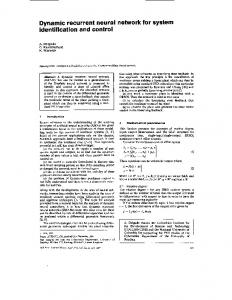
6.1. Nonlinear System Identification. It is assumed that the structure of two-input two-output system is a black box system. In this experiment, this test was to validate the feasibility of the proposed DNN-based identifier to approximate the unknown, coupled, and nonlinear system. In this study, 𝑢1 = 4 sin(0.2𝑡), 𝑢2 = 4 cos(0.6𝑡). The DNN model was selected as follows: ̂ 𝑛𝑛 + 𝐵𝑓 ̂ (𝑥𝑛𝑛 ) + 𝑢 ̇ = 𝐴𝑥 𝑥𝑛𝑛

(46)

which was structured with single layer, 2 neurons and the activation functions were selected as hyperbolic tangent; namely, tanh(𝑥) = (𝑒𝑥 − 𝑒−𝑥 )/(𝑒𝑥 + 𝑒−𝑥 ). Assigned the 50 ̂ and 𝐵(0) ̂ as null matrices, Λ 𝑖 = [ 6000 initials 𝐴(0) 50 6000 ], 𝜎1 = 0.1, and 𝜎2 = 0.02. Then run the online identification procedure and the whole process was run for 50s. The identification results are shown in Figures 5 and 6. The real system (45) is a coupled nonlinear system, and the DNN model (46) is constructed without coupling. We use the DNN (46) to approximate the real system (45) on the basis of the weights updating laws (12) which is derived by the Lyapunov method. In Figures 5 and 6, 𝑥1 and 𝑥2 are the state variables of the real system, 𝑥𝑛𝑛1 and 𝑥𝑛𝑛2 are the state variables of the DNN model, and 𝐸1 and 𝐸2 stand for the errors of state variables between the real system and the DNN model. We can explicitly see that the errors are small enough and the effectiveness of the DNN model according to the relevant algorithm although the DNN model has no coupling features.

−2 −3 −4

0

5

10

15

20

25

30

35

40

45

50

x2 xnn2 E2

Figure 6: Identification result for system state 𝑥2 .

6.2. Nonlinear System Control. Although the DNN has the ability to approximate any nonlinear systems, however, the DNN model errors and environment disturbances are inevitable in the real systems. In the control point of view, we should consider these factors which include neural network model errors and uncertain disturbance forces acting on the real nonlinear systems. The control objective is to make the real outputs of the unknown, coupled, and MIMO nonlinear systems tracking the perspecified inputs; namely, the system states 𝑥 = [𝑥1 , 𝑥2 ]𝑇 to follow the prespecified inputs 𝑥𝑑 = [𝑥𝑑1 , 𝑥𝑑2 ]𝑇 . So a comprehensive control scheme was shown in Section 4, and the controller designed could deal with the compensation of the nonlinearity, the uncertain model errors, and environment disturbances.

8

Abstract and Applied Analysis 3

3

2.5

2.5

2

2

1.5

1.5

1

1

0.5

0.5

0

0

−0.5

−0.5

0

5

10

15

20

25

30

0

5

10

15

20

25

30

x2 xd2 Ed2

x1 xd1 Ed1

Figure 7: Trajectory tracking result for system state 𝑥1 .


In the view of this paper, the real systems can be formulated as

in the response curves. It is concluded that the proposed adaptive controller is able to achieve excellent dynamic performance and high antidisturbance capability in trajectory tracking, which agrees with our theoretic prediction. For the purpose of verifying the generality and effectiveness of the proposed method for more complex nonlinear signal, we choose another reference input signal as follows:

̂ (𝑥𝑛𝑛 ) + 𝑢 + 𝑔̃ (𝑡) , ̂ 𝑛𝑛 + 𝐵𝑓 𝑥̇ = 𝐴𝑥

(47)

where 𝑔̃ = (𝑔̃1 , 𝑔̃2 )𝑇 represents the lump model errors and disturbances. In this study, first we simply define 𝑔̃1 = 0.8 sin(𝑡), 𝑔̃2 = 1.5 cos(𝑡) and the reference model inputs are defined as 0.2 { { ̇ = {sin (0.7𝑡) ̇ = 𝑥𝑑2 𝑥𝑑1 { {0

0 ≤ 𝑡 ≤ 10 10 ≤ 𝑡 ≤ 20 20 ≤ 𝑡.

̇ = cos 𝑡. 𝑥𝑑2 (48)

In fact, the desired inputs 𝑥𝑑1 and 𝑥𝑑2 are the piecewise functions of ramp signal, cosine signal, and step signal. By using the DNN-based identifier to approximate the real systems, the adaptive controller is designed as follows: ̂ 𝑛𝑛 − 𝐵𝑓 ̂ (𝑥𝑛𝑛 ) + ℎ𝑑 , 𝑢𝑐 = −𝐴𝑥 𝑢𝑟 = −𝑘0 ⋅ 𝐸𝑑 − diag (sgn (𝐸𝑑 )) ⋅ 𝑑̂

̇ = sin 𝑡, 𝑥𝑑1

(49)

̂̇ = 󵄩󵄩󵄩𝐸 󵄩󵄩󵄩 . 𝑑 󵄩 𝑑󵄩 ̂ and 𝐵(0) ̂ as null matriAssigned the initials 𝐴(0) 50 ], 𝜎 = 0.1, 𝜎 = 0.02, and 𝑘 = 25. Then ces, Λ 𝑖 = [ 6000 1 2 0 50 6000 run the proposed controller design procedure and the whole process was run for 30 s. The response curves of trajectory tracking are shown in Figures 7 and 8. In Figures 7 and 8, 𝑥1 and 𝑥2 are the state variables identified by DNN model, 𝑥𝑑1 and 𝑥𝑑2 are the reference input signals, and 𝐸𝑑1 and 𝐸𝑑2 stand for the errors of trajectory tracking. We can see no matter how the reference input signals change; 𝐸𝑑1 and 𝐸𝑑2 are bounded as time goes by when considering the model errors and environment disturbances. At the same time, there is no large magnitude of overshoot

(50)

The lump model errors and disturbances 𝑔̃𝑖 are defined as the square signals 𝑔̃1 = 4 square (0.5, 𝑡) , 𝑔̃2 = 3 square (1, 𝑡) .

(51)

And the other conditions are the same with the above. The response curves of trajectory tracking are shown in Figures 9 and 10. From Figures 9 and 10, there is explicitly fluctuation in the first 20 s, but the errors are always bounded and become smaller and smaller as time goes on. And the simulation results once again demonstrate the effectiveness of the proposed control scheme, and it can be observed with the excellent performance of the system states following the prespecified inputs.

7. Conclusion In this paper, we present the DNN identification and adaptive control strategy for the real systems which is of nonlinearity, coupling, and uncertain environment disturbances. According to the Lyapunov methodology, the weights updating laws of DNN-based identifier and the control laws of indirect adaptive controller have been derived to ensure the stability


9 the National Key Basic Research and Development Program of China (973 Program) (no. 2012CB215202).

1.5 1

References

0.5 0 −0.5 −1 −1.5

0

5

10

15

20

25

30

35

40

45

50

x1 xd1 Ed1


1.5 1 0.5 0 −0.5 −1 −1.5

0

5

10

15

20

25

30

35

40

45

50

x2 xd2 Ed2


of decoupling control and to achieve favorable tracking performance for the real system. The simulation results have indicated that the success of decoupling and the proper dynamic response of the plant states to follow the desired input trajectories.

Conflict of Interests The authors declare that there is no conflict of interests regarding the publication of this paper.

Acknowledgments This work was supported by the Fundamental Research Funds for the Central Universities (no. CDJZR10170007) and

[1] X. Z. Wang, “A Summary of multivariable decoupling methods,” Journal of Shenyang Architectural and Civil Engineering, vol. 16, no. 2, pp. 143–145, 2000. [2] T. Y. Chai, S. J. Lang, and X. Y. Gu, “A generalized selftuning feed forward controller and multivariable application,” in Processings of 24th IEEE Conference on Decision and Control, pp. 862–867, 1985. [3] B. Wittenmark, R. H. Middleton, and G. C. Goodwin, “Adaptive decoupling of multivariable systems,” International Journal of Control, vol. 46, no. 6, pp. 1993–2009, 1987. [4] W. J. Mao and J. Chu, “Input-output energy decoupling of linear time-invariant systems,” Control Theory & Applications, vol. 19, no. 1, pp. 146–148, 2002. [5] X. Z. Dong and Q. L. Zhang, “Input-output energy decoupling of linear singular systems,” Journal of Northeastern University, vol. 25, no. 6, pp. 523–526, 2004. [6] Z. Gao, “Active disturbance rejection control: a paradigm shift in feedback control system design,” in Proceedings of the American Control Conference, pp. 2399–2405, June 2006. [7] Q. Zheng, Z. Chen, and Z. Gao, “A practical approach to disturbance decoupling control,” Control Engineering Practice, vol. 17, no. 9, pp. 1016–1025, 2009. [8] T. E. Djaferis, Robust Decoupling for Systems With Parameters Modeling, Identification and Robust Control, B V NorthHolland, Elsevier Science, 1986. [9] G. Z. Pang and Z. Y. Chen, “The relation between robust stability and robust diagonal dominance,” Acta Atuomatic Sinica, vol. 18, no. 3, pp. 273–281, 1992. [10] T. H. Lee, J. H. Nie, and M. W. Lee, “A fuzzy controller with decoupling for multivariable nonlinear servo-mechanisms, with application to real-time control of a passive line-of-sight stabilization system,” Mechatronics, vol. 7, no. 1, pp. 83–104, 1997. [11] H. Li, “Design of multivariable fuzzy-neural network decoupling controller,” Kongzhi yu Juece/Control and Decision, vol. 21, no. 5, pp. 593–596, 2006. [12] J. Maldacena, “The large-𝑁 limit of superconformal field theories and supergravity,” International Journal of Theoretical Physics, vol. 38, no. 4, pp. 1113–1133, 1999, Quantum gravity in the southern cone (Bariloche, 1998). [13] Y. B. Dai, W. D. Yang, and S. F. Wang, “A summary of multivariable predictive decoupling control methods,” Electrical Automation, vol. 30, no. 6, pp. 1–3, 2008. [14] R. Pothin, “Disturbance decoupling for a class of nonlinear MIMO systems by static measurement feedback,” Systems & Control Letters, vol. 43, no. 2, pp. 111–116, 2001. [15] Q. X. Gong, Research on disturbance decoupling and attenuation control for nonlinear systems, [Doctor dissertation of Northeastern University], 2008. [16] L. M. Wu and T. Y. Chai, “A neural network decoupling strategy for a class of nonlinear discrete time systems,” Acta Atuomatic Sinica, vol. 23, no. 2, pp. 207–212, 1997. [17] X. Su, P. Shi, L. Wu, and Y. D. Song, “Novel control design on discrete-time Takagi-Sugeno fuzzy systems with time-varying delays,” IEEE Transactions on Fuzzy Systems, vol. 20, no. 6, pp. 655–671, 2013.

10 [18] K. S. Narendra and K. Parthasarathy, “identification and control of dynamical systems using neural networks,” IEEE Transactions on Neural Networks, vol. 1, no. 1, pp. 4–27, 1990. [19] M. M. Gupta and D. H. Rao, Neuro-Control Systems: Theory and Applications, IEEE Press, Piscataway, NJ, USA, 1994. [20] K. Hunt, G. Irwin, and K. Warwick, Neural Networks Engineering in Dynamic Control Systems: Advances in Industrial Control, Springer, New York, NY, USA, 1995. [21] Y. Kourd, D. Lefebvre, and N. Guersi, “Fault diagnosis based on neural networks and decision trees: application to DAMADICS,” International Journal of Innovative Computing, Information and Control, vol. 9, no. 8, pp. 3185–3196, 2013. [22] P. L. Liu, “Delay-dependent robust stability analysis for recurrent neural networks with time-varying delay,” International Journal of Innovative Computing, Information and Control, vol. 9, no. 8, pp. 3341–3355, 2013. [23] S. Sefriti, J. Boumhidi, M. Benyakhlef, and I. Boumhidi, “Adaptive decentralized sliding mode neural network control of a class of nonlinear interconnected systems,” International Journal of Innovative Computing, Information and Control, vol. 9, no. 7, pp. 2941–2947, 2013. [24] X. Su, Z. Li, Y. Feng, and L. Wu, “New global exponential stability criteria for interval-delayed neural networks,” Proceedings of the Institution of Mechanical Engineers I: Journal of Systems and Control Engineering, vol. 225, no. 1, pp. 125–136, 2011. [25] C.-H. Wang, P.-C. Chen, P.-Z. Lin, and T.-T. Lee, “A dynamic neural network model for nonlinear system identification,” in Proceedings of the IEEE International Conference on Information Reuse and Integration, IRI 2009, pp. 440–441, August 2009. [26] X.-J. Wu, Q. Huang, and X.-J. Zhu, “Power decoupling control of a solid oxide fuel cell and micro gas turbine hybrid power system,” Journal of Power Sources, vol. 196, no. 3, pp. 1295–1302, 2011. [27] Z. J. Fu, W. F. Xie, X. Han, and W. D. Luo, “Nonlinear system identification and control via dynamic multitime scales neural networks,” IEEE Transactions on Neural Networks and Learning Systems, vol. 24, no. 11, pp. 1814–1823, 2013.


Advances in

Operations Research Hindawi Publishing Corporation http://www.hindawi.com

Volume 2014

Advances in

Decision Sciences Hindawi Publishing Corporation http://www.hindawi.com

Volume 2014

Journal of

Applied Mathematics

Algebra

Hindawi Publishing Corporation http://www.hindawi.com


Volume 2014

Journal of

Probability and Statistics Volume 2014

The Scientific World Journal Hindawi Publishing Corporation http://www.hindawi.com


Volume 2014

International Journal of

Differential Equations Hindawi Publishing Corporation http://www.hindawi.com

Volume 2014

Volume 2014

Submit your manuscripts at http://www.hindawi.com International Journal of

Advances in

Combinatorics Hindawi Publishing Corporation http://www.hindawi.com

Mathematical Physics Hindawi Publishing Corporation http://www.hindawi.com

Volume 2014

Journal of

Complex Analysis Hindawi Publishing Corporation http://www.hindawi.com

Volume 2014

International Journal of Mathematics and Mathematical Sciences

Mathematical Problems in Engineering

Journal of

Mathematics Hindawi Publishing Corporation http://www.hindawi.com

Volume 2014


Volume 2014

Volume 2014


Volume 2014

Discrete Mathematics

Journal of

Volume 2014


Discrete Dynamics in Nature and Society

Journal of

Function Spaces Hindawi Publishing Corporation http://www.hindawi.com


Volume 2014


Volume 2014


Volume 2014

International Journal of

Journal of

Stochastic Analysis

Optimization



Volume 2014

Volume 2014