Reservoir Computing for Learning in Structured ...

` di Pisa Universita

Dipartimento di Informatica Dottorato di Ricerca in Informatica

Ph.D. Thesis

Reservoir Computing for Learning in Structured Domains (SSD) INF 01 Claudio Gallicchio

Supervisor Alessio Micheli

November 10, 2011

Abstract The study of learning models for direct processing complex data structures has gained an increasing interest within the Machine Learning (ML) community during the last decades. In this concern, efficiency, effectiveness and adaptivity of the ML models on large classes of data structures represent challenging and open research issues. The paradigm under consideration is Reservoir Computing (RC), a novel and extremely efficient methodology for modeling Recurrent Neural Networks (RNN) for adaptive sequence processing. RC comprises a number of different neural models, among which the Echo State Network (ESN) probably represents the most popular, used and studied one. Another research area of interest is represented by Recursive Neural Networks (RecNNs), constituting a class of neural network models recently proposed for dealing with hierarchical data structures directly. In this thesis the RC paradigm is investigated and suitably generalized in order to approach the problems arising from learning in structured domains. The research studies described in this thesis cover classes of data structures characterized by increasing complexity, from sequences, to trees and graphs structures. Accordingly, the research focus goes progressively from the analysis of standard ESNs for sequence processing, to the development of new models for trees and graphs structured domains. The analysis of ESNs for sequence processing addresses the interesting problem of identifying and characterizing the relevant factors which influence the reservoir dynamics and the ESN performance. Promising applications of ESNs in the emerging field of Ambient Assisted Living are also presented and discussed. Moving towards highly structured data representations, the ESN model is extended to deal with complex structures directly, resulting in the proposed TreeESN, which is suitable for domains comprising hierarchical structures, and GraphESN, which generalizes the approach to a large class of cyclic/acyclic directed/undirected labeled graphs. TreeESNs and GraphESNs represent both novel RC models for structured data and extremely efficient approaches for modeling RecNNs, eventually contributing to the definition of an RC framework for learning in structured domains. The problem of adaptively exploiting the state space in GraphESNs is also investigated, with specific regard to tasks in which input graphs are required to be mapped into flat vectorial outputs, resulting in the GraphESN-wnn and GraphESN-NG models. As a further point, the generalization performance of the proposed models is evaluated considering both artificial and complex real-world tasks from different application domains, including Chemistry, Toxicology and Document Processing.

4

This thesis is dedicated to my family.

6

And now you’re mine. Rest with your dream in my dream. Love and pain and work should all sleep, now. The night turns on its invisible wheels, and you are pure beside me as a sleeping amber. No one else, Love, will sleep in my dreams. You will go, we will go together, over the waters of time. No one else will travel through the shadows with me, only you, evergreen, ever sun, ever moon. Your hands have already opened their delicate fists and let their soft drifting signs drop away, your eyes closed like two gray wings, and I move after, following the folding water you carry, that carries me away: the night, the world, the wind spin out their destiny, without you, I am your dream, only that, and that is all.

Pablo Neruda (Love Sonnet LXXXI) (To every sunrise, and every sunset, until you are mine, thesis).

Acknowledgments I whish to thank my supervisor, Alessio Micheli, for his help and support during these years. Alessio, you have been my guide: I am in your debt. It has been a pleasure to work with you. Going on with this work will be an honor. I thank Peter Tiˇ no and Ah Chung Tsoi, the reviewers of this thesis, for their precious suggestions and considerations which improved the quality of this work. I am also grateful to the coordinator of the graduate study program, Pierpaolo Degano and to the members of my thesis commettee, Paolo Mancarella and Salvatore Ruggieri. I also thank all the co-authors of the works which contributed to this thesis.

Ringraziamenti Personali In questi anni di dottorato a Pisa ho imparato diverse cose: sulla scienza, sulle persone, su me stesso. Per esempio ho imparato che spesso poche parole giuste funzionano meglio di molte parole inutili. Quindi grazie. Grazie mamma, grazie pap` a, grazie Germano. Non ho parole per ringraziarvi del supporto che mi avete dato incondizionatamente in questi anni. Non sono stati sempre facili, questi anni. Non per me e non per voi. Dal profondo del mio cuore e dei miei occhi, grazie. Grazie anche a tutta la mia famiglia, ai miei nonni, alle zie e agli zii, alle cugine e ai cugini. Avere un punto fisso cos`ı non capita in ogni vita. Per questo mi sento e mi sono sentito sempre un fortunato. Grazie anche a tutti i compagni di avventura con i quali ho condiviso questa esperienza del dottorato (e anche molte notti insonni). Grazie a tutte le persone con le quali ho parlato del mio lavoro. In ogni modo e in ogni luogo. Grazie anche a tutti quelli che non mi hanno fatto parlare del mio lavoro. Grazie a tutti i miei amici, per l’incoraggiamento costante che mi hanno dato e che continuano a darmi. Quando sono stato felice e quando sono stato triste, sempre, siete stati una risorsa preziosa. Spesso, una fortuna insperata. Infine ringrazio anche te, che forse non leggerai mai queste parole. La maggior parte dei lavori che compaiono in questa tesi li ho scritti dividendo la mia vita con te. Ci sono molti modi in cui vorrei ringraziarvi. Sapr` o farlo, oltre queste parole. Grazie.

8

Contents I

Basics

1 Introduction 1.1 Motivations . . . . . . . . . 1.2 Objectives of the Thesis . . 1.3 Contributions of the Thesis 1.4 Plan of the Thesis . . . . . 1.5 Origin of the Chapters . . .

13 . . . . .

. . . . .

. . . . .

. . . . .

. . . . .

. . . . .

. . . . .

15 15 17 18 21 22

2 Background and Related Works 2.1 Machine Learning for Flat Domains . . . . . . . . . . . . . . . . 2.1.1 A Short Introduction to Machine Learning . . . . . . . . 2.1.2 Learning and Generalization . . . . . . . . . . . . . . . . 2.1.3 Feed-forward Neural Networks . . . . . . . . . . . . . . . 2.1.4 Support Vector Machines and Kernel Methods . . . . . . 2.1.5 Nearest Neighbor . . . . . . . . . . . . . . . . . . . . . . . 2.1.6 Neural Gas . . . . . . . . . . . . . . . . . . . . . . . . . . 2.2 Neural Networks for Learning in Structured Domains . . . . . . . 2.2.1 A General Framework for Processing Structured Domains 2.2.2 Recursive Processing of Transductions on Sequences . . . 2.2.3 Recursive Processing of Transductions on Trees . . . . . . 2.2.4 Recurrent Neural Networks . . . . . . . . . . . . . . . . . 2.2.5 Reservoir Computing and Echo State Networks . . . . . . 2.2.6 Recursive Neural Networks . . . . . . . . . . . . . . . . . 2.2.7 Related Approaches . . . . . . . . . . . . . . . . . . . . .

. . . . . . . . . . . . . . .

. . . . . . . . . . . . . . .

. . . . . . . . . . . . . . .

. . . . . . . . . . . . . . .

. . . . . . . . . . . . . . .

. . . . . . . . . . . . . . .

23 24 24 26 28 30 33 34 36 36 43 44 46 47 52 56

. . . . .

. . . . .

. . . . .

. . . . .

. . . . .

. . . . .

. . . . .

. . . . .

. . . . .

. . . . .

. . . . .

. . . . .

. . . . .

. . . . .

. . . . .

. . . . .

. . . . .

. . . . .

. . . . .

. . . . .

II Analysis and Applications of Reservoir Computing for Sequence Domains 61 3 Markovian and Architectural Factors of 3.1 Introduction . . . . . . . . . . . . . . . . 3.2 Echo State Property and Contractivity . 3.3 Markovian Factor of ESNs . . . . . . . . 3.4 Architectural Factors of ESN Design . . 3.5 Experimental Results . . . . . . . . . . . 3.5.1 Tasks . . . . . . . . . . . . . . .

ESN dynamics . . . . . . . . . . . . . . . . . . . . . . . . . . . . . . . . . . . . . . . . . . . . . . . . . . . . . . . . . . . .

. . . . . .

. . . . . .

. . . . . .

. . . . . .

. . . . . .

. . . . . .

. . . . . .

. . . . . .

. . . . . .

. . . . . .

63 63 65 67 70 74 75

10

CHAPTER 0. CONTENTS

3.6

3.5.2 Markovian Factor Results . . . . . . . . . . . . . . . . . . . . . . . . 78 3.5.3 Architectural Factors Results . . . . . . . . . . . . . . . . . . . . . . 83 Conclusions . . . . . . . . . . . . . . . . . . . . . . . . . . . . . . . . . . . . 98

4 A Markovian Characterization of Redundancy in ESNs 4.1 Introduction . . . . . . . . . . . . . . . . . . . . . . . . . . 4.2 Principal Component Analysis of Echo State Networks . . 4.3 Conclusions . . . . . . . . . . . . . . . . . . . . . . . . . . 5 Applications of ESNs for Ambient Assisted Living 5.1 Introduction . . . . . . . . . . . . . . . . . . . . . . . 5.2 Related work . . . . . . . . . . . . . . . . . . . . . . 5.3 Experiments in Homogeneous Indoor Environment . 5.3.1 Slow Fading Analysis . . . . . . . . . . . . . . 5.3.2 Computational Experiments . . . . . . . . . . 5.4 Experiments in Heterogeneous Indoor Environments 5.4.1 Computational Experiments . . . . . . . . . . 5.5 Conclusions . . . . . . . . . . . . . . . . . . . . . . .

III

. . . . . . . .

. . . . . . . .

. . . . . . . .

by . . . . . .

. . . . . . . .

. . . . . . . .

PCA . . . . . . . . . . . . . . . . . . . . .

105 . 105 . 105 . 109

. . . . . . . .

111 . 111 . 112 . 114 . 114 . 116 . 122 . 123 . 124

. . . . . . . .

. . . . . . . .

. . . . . . . .

. . . . . . . .

. . . . . . . .

. . . . . . . .

Reservoir Computing for Highly Structured Domains

127

6 Tree Echo State Networks 129 6.1 Introduction . . . . . . . . . . . . . . . . . . . . . . . . . . . . . . . . . . . . 129 6.2 TreeESN Model . . . . . . . . . . . . . . . . . . . . . . . . . . . . . . . . . . 130 6.2.1 Reservoir of TreeESN . . . . . . . . . . . . . . . . . . . . . . . . . . 130 6.2.2 State Mapping Function: TreeESN-R and TreeESN-M . . . . . . . . 133 6.2.3 Readout of TreeESN . . . . . . . . . . . . . . . . . . . . . . . . . . . 133 6.2.4 Markovian Characterization and Initialization of Reservoir Dynamics 134 6.2.5 Computational Complexity of TreeESNs . . . . . . . . . . . . . . . . 138 6.3 Experiments . . . . . . . . . . . . . . . . . . . . . . . . . . . . . . . . . . . . 139 6.3.1 INEX2006 Task . . . . . . . . . . . . . . . . . . . . . . . . . . . . . . 140 6.3.2 Markovian/anti-Markovian Tasks . . . . . . . . . . . . . . . . . . . . 142 6.3.3 Alkanes Task . . . . . . . . . . . . . . . . . . . . . . . . . . . . . . . 145 6.3.4 Polymers Task . . . . . . . . . . . . . . . . . . . . . . . . . . . . . . 149 6.4 Conclusions . . . . . . . . . . . . . . . . . . . . . . . . . . . . . . . . . . . . 153 7 Graph Echo State Networks 7.1 Introduction . . . . . . . . . . . . . . 7.2 GraphESN Model . . . . . . . . . . . 7.2.1 Reservoir of GraphESN . . . 7.2.2 State Mapping Function . . . 7.2.3 Readout of GraphESN . . . . 7.2.4 Computational Complexity of 7.3 Experiments . . . . . . . . . . . . . . 7.3.1 Experimental Settings . . . . 7.3.2 Results . . . . . . . . . . . .

. . . . . . . . . . . . . . . . . . . . . . . . . . . . . . . . . . . GraphESNs . . . . . . . . . . . . . . . . . . . . .

. . . . . . . . .

. . . . . . . . .

. . . . . . . . .

. . . . . . . . .

. . . . . . . . .

. . . . . . . . .

. . . . . . . . .

. . . . . . . . .

. . . . . . . . .

. . . . . . . . .

. . . . . . . . .

. . . . . . . . .

. . . . . . . . .

. . . . . . . . .

155 . 155 . 156 . 158 . 165 . 165 . 166 . 167 . 168 . 169

11

0.0. CONTENTS

7.4

Conclusions . . . . . . . . . . . . . . . . . . . . . . . . . . . . . . . . . . . . 171

8 Adaptivity of State Mappings for GraphESN 8.1 Introduction . . . . . . . . . . . . . . . . . . . . . . . . . . . . . . 8.2 GraphESN-wnn: Exploiting Vertices Information Using Weighted 8.2.1 Experimental Results . . . . . . . . . . . . . . . . . . . . 8.3 GraphESN-NG: Adaptive Supervised State Mapping . . . . . . . 8.3.1 Experimental Results . . . . . . . . . . . . . . . . . . . . 8.4 Conclusions . . . . . . . . . . . . . . . . . . . . . . . . . . . . . .

. . . . K-NN . . . . . . . . . . . . . . . .

. . . . . .

9 Conclusions and Future Works A Datasets A.1 Markovian/Anti-Markovian Symbolic Sequences . A.2 Engine Misfire Detection Problem . . . . . . . . A.3 Mackey-Glass Time Series . . . . . . . . . . . . . A.4 10-th Order NARMA System . . . . . . . . . . . A.5 Santa Fe Laser Time Series . . . . . . . . . . . . A.6 AAL - Homogeneous Indoor Environment . . . . A.7 AAL - Heterogeneous Indoor Environments . . . A.8 INEX2006 . . . . . . . . . . . . . . . . . . . . . . A.9 Markovian/anti-Markovian Symbolic Trees . . . A.10 Alkanes . . . . . . . . . . . . . . . . . . . . . . . A.11 Polymers . . . . . . . . . . . . . . . . . . . . . . A.12 Mutagenesis . . . . . . . . . . . . . . . . . . . . . A.13 Predictive Toxicology Challenge (PTC) . . . . . A.14 Bursi . . . . . . . . . . . . . . . . . . . . . . . . . Bibliography

. . . . . .

173 173 174 176 176 179 180 183

. . . . . . . . . . . . . .

. . . . . . . . . . . . . .

. . . . . . . . . . . . . .

. . . . . . . . . . . . . .

. . . . . . . . . . . . . .

. . . . . . . . . . . . . .

. . . . . . . . . . . . . .

. . . . . . . . . . . . . .

. . . . . . . . . . . . . .

. . . . . . . . . . . . . .

. . . . . . . . . . . . . .

. . . . . . . . . . . . . .

. . . . . . . . . . . . . .

. . . . . . . . . . . . . .

189 . 189 . 190 . 190 . 191 . 191 . 192 . 193 . 194 . 195 . 196 . 197 . 198 . 199 . 199 201

12

CHAPTER 0. CONTENTS

Part I

Basics

Chapter 1

Introduction 1.1

Motivations

Traditional Machine Learning (ML) models are suitable for dealing with flat data only, such as vectors or matrices. However, in many real-world applicative domains, including e.g. Cheminformatics, Molecular Biology, Document and Web processing, the information of interest can be naturally represented by the means of structured data representations. Structured data, such as sequences, trees and graphs, are indeed inherently able to describe the relations existing among the basic entities under consideration. Moreover, the problems of interest can be modeled as regression or classification tasks on such structured domains. For instance, when dealing with Chemical information, molecules can be suitably represented as graphs, where vertices stand for atoms and edges stand for bonds between atoms. Accordingly, problems such as those in the field of toxicity prediction can be modeled as classification tasks on such graph domains. When approaching real-world problems, standard ML methods often need to resort to fixed-size vectorial representations of the input data under consideration. This approach, however, implies several drawbacks such as the possibility of loss of the relational information within the original data and the necessity of domain experts to design such fixed representations in an a-priori and task specific fashion. In light of these considerations, it seems conceivable that the generalization of ML for processing structured information directly, also known as learning in structured domains, has increasingly attracted the interest of researchers in the last years. However, when structured data are considered, along with a natural richness of applicative tasks that can be approached in a more suitable and direct fashion, several research problems emerge, mainly related to the increased complexity of the data domains to be treated. A number of open issues still remain and motivate the investigations described in this thesis. First of all, efficiency of the learning algorithms is identified as one of the most relevant aspects deserving particular attention under both theoretical and practical points of view. Moreover, the generalization of the class of data structures that can be treated directly is of a primary interest in order to extend the expressiveness and the applicability of the learning models from sequences, to trees and graphs. Finally, when dealing with structured information, adaptivity and generalization ability of the ML models represent further critical points. In this thesis we mainly deal with neural networks, which constitute a powerful class

16

CHAPTER 1. INTRODUCTION

of ML models, characterized by desirable universal approximation properties and successfully applied in a wide range of real-world applications. In particular, Recurrent Neural Networks (RNNs) [121, 178, 94] represent a widely known and used class of neural network models for learning in sequential domains. Basically, the learning algorithms used for training RNNs are extensions of the gradient descending methods devised for feed-forward neural networks. Such algorithms, however, typically involve some known drawbacks such as the possibility of getting stuck in local minima of the error surface, the difficulty in learning long-term dependencies, the slow convergence and the high computational training costs (e.g. [89, 127]). An interesting characterization of RNN state dynamics is related to standard contractive initialization conditions using small weights, resulting in a Markovian architectural bias [90, 176, 175, 177] of the network dynamics. Recently, Reservoir Computing (RC) [184, 127] models in general, and Echo State Networks (ESNs) [103, 108] in particular, are becoming more and more popular as extremely efficient approaches for RNN modeling. An ESN consists in a large non-linear reservoir hidden layer of sparsely connected recurrent units and a linear readout layer. The striking characteristic of ESNs is that the reservoir part can be left untrained after a random initialization under stability constraints, so that the only trained component of the architecture is a linear recurrentfree output layer, resulting in a very efficient approach. Very interestingly, in spite of their extreme efficiency, ESNs achieved excellent results in many benchmark applications (often outperforming state-of-the-art results [108, 103]), contributing to increase the appeal of the approach. Despite its recent introduction, a large literature on the ESN model exists (e.g. see [184, 127] for reviews), and a number of open problems are currently attracting the research interest in this field. Among them, the most studied ones are related to the optimization of reservoirs toward specific applications (e.g. [102, 163, 164]), the topological organization of reservoirs (e.g. [195, 110]), possible simplifications and variants of the reservoir architecture (e.g. [53, 29, 31, 157, 26]), stabilizing issues in presence of output feedback connections (e.g. [156, 109, 193]) and the aspects concerning the short-term memory capacity and non-linearity of the model (e.g. [183, 25, 98, 97]). However, a topic which is often not much considered in the ESN literature regards the characterization of the properties of the model which may influence its success in applications. Studies in this direction are particularly worth of research interest as indeed they can lead to a deeper understanding of the real intrinsic potentialities and limitations of the ESN approach, contributing to a more coherent placement of this model within the field of ML for sequence domains processing. Moreover, although the performance of ESNs in many benchmark problems resulted extremely promising, the effectiveness of ESN networks in complex real-world applications is still considered a matter of investigation, and devising effective solutions for real-world problems using ESNs is often a difficult task [151]. Recursive Neural Networks (RecNNs) [169, 55] are a generalization of RNNs for direct processing hierarchical data structures, such as rooted trees and directed acyclic graphs. RecNNs implement state transition systems on discrete structures, where the output is computed by preliminarily encoding the structured input into an isomorphic structured feature representation. RecNNs allowed to extend the applicability of neural models to a wide range of real-world applicative domains, such as Cheminformatics (e.g. [20, 141, 46, 142]), Natural Language Processing [36, 173] and Image Analysis [54, 39]. In addition to this, a number of results about the capabilities of universal approximation of RecNNs on hierarchical structures have been proved (see [86, 82]). However, the issues related to RNN training continue to hold also for RecNNs [91], in which case the learning algorithms can

1.2. OBJECTIVES OF THE THESIS

17

be even more computationally expensive. Thereby, efficiency represents a very important aspects related to RecNN modeling. Another relevant open topic concerns the class of structures which can be treated by RecNNs, traditionally limited to hierarchical data. Indeed, when dealing with more general structured information with RecNNs, the encoding process in general is not ensured to converge to a stable solution [169]. More in general, enlarging the class of data structures supported to general graphs is an relevant topic in designing neural network models. Resorting to constructive static approaches [139], preprocessing the input structures (e.g. by collapsing cyclic substructures into single vertices, e.g. [142]), or constraining the dynamics of the RecNN to ensure stability [160] are examples of interesting solutions provided in literature, confirming the significance of this topic. The development of novel solutions for learning in highly structured domains based on the RC paradigm represents an exciting and promising research line. Indeed it would allow us to combine the extreme approach to learning of the ESN model, with the richness and the potential of complex data structures. More specifically, RC provides intrinsically efficient solutions to sequence domains processing, and on the other hand it allows us to envisage possible methods to exploit the stability properties of reservoir dynamics in order to enlarge to general graphs the class of data structures supported. Finally, another notable aspect is related to the problem of extracting the relevant information from the structured state space obtained by the encoding process of recursive models on structured data. This problem arises whenever the task at hand requires to map input structures into unstructured vectorial outputs (e.g. in classification of regression tasks on graphs), and assumes a particular relevance whenever we want to be able to deal with variable size and topology input structures, without resorting to fixed vertices alignments. If hierarchical data is considered (e.g. sequences or rooted trees), the selection of the state associated to the supersource of the input structure often represents a meaningful solution. However, for classes of graphs in which the definition of the supersource can be arbitrary, the study of approaches for relevant state information extraction is particularly interesting, also in relation to the other characteristics of the models. Moreover, the development of flexible and adaptive methods for such state information extraction/selection is of a great appeal.

1.2

Objectives of the Thesis

The main objective of this thesis consists in proposing and analyzing efficient RC models for learning in structured domains. In light of their characteristics, the RC in general and the ESN model in particular, are identified as suitable reference paradigms for approaching the complexity and investigating the challenges of structured information processing. Within the main goal, as more complex structured domains are taken into consideration, the focus of the research gradually moves from the analysis of the basic models for sequence domains, to the development of new models for tree and graph domains. In particular, the investigations on the standard ESN focus on the problem of isolating and properly characterizing the main aspects of the model design which define the properties and the limitations of reservoir dynamics and positively/negatively influence the ESN performance in applications. When more complex data structures are considered, the research interest is more prominently focused on devising novel analytical and modeling

18


tools, based on the generalization of ESN to trees and graphs, in order to approach the challenges arising from the increased data complexity. In this concern, an aspect deserving attention is related to the possibility of developing adaptive methods for the extraction of the state information from structured reservoir state spaces. This point is of special interest when dealing with variable size and topology general graphs. At the same time, in our research direction from sequences, to trees, to graphs, the most appropriate tools developed for less general classes of structures are preserved and exploited also for dealing with more general data structures. Overall, the research studies described in this thesis aim at developing an RC framework for learning with increasingly complex and general structured information, providing a set of tools with more specific suitability for specific classes of structures. Another objective consists in assessing the predictive performance of the proposed models on both artificial and challenging real-world tasks, in order to confirm the appropriateness and the effectiveness of the solutions introduced. Such applicative results contribute to enlighten the characteristics and critical points of the approach, which are properly investigated and analyzed.

1.3

Contributions of the Thesis

The main contributions of this thesis are discussed in the following. Analysis of Markovian and architectural factors of ESNs We provide investigations aimed at identifying and analyzing the factors of ESNs which determine the characteristics of the approach and influence successful/unsuccessful applications. Such factors are related to both the initialization conditions of the reservoir and to the architectural design of the model. In particular, the fixed contractive initialized reservoir dynamics implies an intrinsic suffix-based Markovian nature of the state space organization. The study of such Markovian organization of reservoir state spaces constitutes a ground for the analysis of the RC models on structured domains proposed in the following of the thesis. The role of Markovianity results of a particular relevance in defining the characteristics and the limitations of the ESN model, and positively/negatively influences its applicative success. The effect of Markovianity in relation to the known issue of redundancy of reservoir units activations is also studied. Other important aspects, such as high dimensionality and non-linearity of the reservoir, are analyzed to isolate the architectural sources of richness of ESN dynamics. Specifically, the roles of variability on the input, on the time-scale dynamics implemented and on the interaction among the reservoir units reveal relevant effects in terms of diversification among the reservoir units activations. In addition, the possibility of applying a linear regression model in a high dimensional reservoir state space is considered as another major factor in relation to the usual high dimensionality of the reservoir. Architectural variants of the standard ESN model are also accordingly introduced. Their predictive performance is experimentally assessed in benchmark and complex real-world tasks, in order to highlight the effects of the inclusion in the ESN design of single factors, of their combinations and their relative importance.

1.3. CONTRIBUTIONS OF THE THESIS

19

Tree Echo State Networks We introduce the Tree Echo State Network (TreeESN) model, an extension of the ESN for processing rooted tree domains. As such, TreeESN represents also an extremely efficient approach for modeling RecNNs. The computational cost of TreeESN is properly analyzed and discussed. The generalized reservoir of TreeESNs encodes each input tree into a state representation whose structure is isomorphic to the structure of the input1 . The tree structured state computed by the reservoir is then used to feed the readout for output computation. We provide an analysis of the initialization conditions based on contractivity of the dynamics of the state transition system implemented on tree patterns. The resulting Markovian characterization of the reservoir dynamics represents an important aspect of investigation, inherited from our studies on standard RC models, extended to the case of tree suffixes. For applications in which a single vectorial output is required in correspondence of each input tree (e.g. for classification of trees), we introduce the notion of the state mapping function, which maps a structured state into a fixed-size feature state representation to which the readout can be applied in order to compute the output. Two choices for the state mapping function are proposed and investigated, namely we consider a root state mapping (selecting the state of the root node) and a mean state mapping (which averages the state information over all the nodes in an input tree). The effects of the choice of the state mapping function are studied both theoretically and experimentally. In particular, an aspect of great importance for applications of TreeESNs is the study of the relations between the choice of the state mapping function and the characteristics of the target task to approach. The potential of the model in terms of applicative success is assessed through experiments on a challenging real-world Document Processing task from an international competition, showing that TreeESN, in spite of its efficiency, can represent an effective solution capable of outperforming state-of-the-art approaches for tree domain processing. Graph Echo State Networks The Graph Echo State Network (GraphESN) model generalizes the RC paradigm for a large class of cyclic/acyclic directed/undirected labeled graphs. GraphESNs are therefore introduced according to the two aspects of efficiently designing RecNNs and enlarging the class of data structures naturally supported by recursive neural models. A contractive initialization condition is derived for GraphESN, representing a generalization of the analogous conditions for ESNs and TreeESNs. The role of contractivity in this case represents also the basis for reservoir dynamics stabilization on general graph structures, even in the case of cyclic and undirected graphs, resulting in an iterative encoding process whose convergence to a unique solution is guaranteed. The Markovian organization of reservoir dynamics, implied by contractivity, is analyzed also for GraphESN, characterizing its inherent ability to discriminate among different input graph patterns in a suffix-based vertex-wise fashion. In this concern, the concept of suffix is also suitably generalized to the case of graph processing. In this sense, the GraphESN model turns out to be an architectural baseline for recursive models, especially for those based on trained contractive 1

The notion of isomorphism here is related to the (variable) topological structure of the input tree. This point is elaborated in Sections 2.2.1, 2.2.3 and 6.2 (see also [86]), and is inherited from the concept of synchronous sequence transductions processing [55].

20


state dynamics. The efficiency of GraphESN is studied through the analysis of its computational cost, which is also interestingly compared with those of state-of-the-art learning models for structured data. The role of the state mapping function in GraphESNs is even more relevant, in particular when dealing with classes of general graphs, for which a supersource or a topological order on the vertices cannot be defined. Experiments on real-world tasks show the effectiveness of the GraphESN approach for tasks on graph domains.

Adaptive and supervised extraction of information from structured state spaces: GraphESN-wnn and GraphESN-NG The study of recursive models on general graph domains highlights the problems related to the fixed metrics adopted in the computation of state mapping functions, representing an issue still little investigated in literature. Thereby, for tasks requiring to map input graphs into fixed-size vectorial outputs, we study the problem of extracting the relevant state information from structured reservoir state spaces. The relevance of this problem is also related to the necessity of processing variable size and topology graph domains, without resorting to fixed alignments of the vertices. We approach this problem by focusing our research on flexible and adaptive implementations of the state mapping function, making use of state-of-the-art ML methods. In the progressive modeling improvement of GraphESN towards adaptivity of the state mapping function, we introduce the GraphESNwnn and the GraphESN-NG models. In particular, GraphESN-wnn uses a variant of the distance-weighted nearest neighbor algorithm to extract the state information in a supervised but non-adaptive fashion. On the other hand, in GraphESN-NG the reservoir state space is clustered using the Neural Gas algorithm, so that the state information is locally decomposed and then combined based on the target information, realizing an adaptive state mapping function. The effectiveness of processing the state information in a flexible and target-dependent way is experimentally shown on real-world tasks. Real-world applications Finally, in this thesis we also present interesting applications of RC models to realworld tasks. In the context of sequence processing, we show an application of ESNs in the innovative emergent field of Ambient Assisted Living. In this case the RC approach is used to forecast the movements of users based on the localization information provided by a Wireless Sensor Network. Moving to more complex data structures, we show the application of TreeESN and GraphESN (including also GraphESN-wnn and GraphESN-NG) to a number of real-world problems from Cheminformatics, Toxicology and Document Processing domains. In this regard, it is worth stressing that despite the fact that TreeESN and GraphESN are designed to cover increasingly general class of structures, each model is specifically more suitable for specific classes of structures. In particular, when the information of interest for the problem at hand can be coherently represented by rooted trees, the TreeESN model provides an extremely efficient yet effective solution, with performance in line with other state-of-the-art methods for tree domains. In other cases, when the data is more appropriately representable by the means of general (possibly cyclic and undirected) graphs, the GraphESN model, preserving the efficiency of the approach, represent the natural RC solution.

1.4. PLAN OF THE THESIS

1.4

21

Plan of the Thesis

This thesis is organized in three parts. In Part I (Chapter 2), we present a review of the basic notions of ML which are of specific interest for this thesis. In Section 2.1 we briefly describe standard ML methods for processing flat domains, with particular regard to neural network models for supervised learning. Then, in Section 2.2, we focus the attention on ML for structured domains. In particular, we introduce the general framework for recursive processing structured domains that is referred in the rest of the thesis. The classes of RNNs and RecNNs, the RC paradigm and the related approaches are described within such framework. As specified in Section 1.2, in this thesis we consider classes of data structures of progressive complexity and generality, from sequences, to trees and graphs, with a research focus that consequently moves from analysis to development of new models. For the sake of simplicity of the organization, although the studies described follow a uniform line of research, the investigations on the standard ESN for sequence processing are described in Part II, while the studies concerning the generalization of the RC paradigm for highly structured domains are described in Part III. More in detail, in Part II, Chapter 3 presents the analysis of the Markovian and architectural factors of ESN design. In particular, the effect of the Markovian nature of the reservoir state space organization is discussed, and relevant factors of ESN architectural design are introduced along with corresponding variants to the standard ESN model. Chapter 4 investigates the relations between Markovianity of ESN dynamics and the issue of redundancy among reservoir units activations. Finally, Chapter 5 illustrates an application of ESNs in the area of Ambient Assisted Living. Part III presents the studies related to the generalization of the RC paradigm to highly structured domains. Chapter 6 introduces the TreeESN model. The study of Markovianity, inherited from the investigations on sequence domains in Part II, is adopted as a useful tool for characterizing the properties of the proposed model. Chapter 6 also introduces the concept of state mapping functions for structured domain processing within the RC approach, illustrating its relations with the characteristics of the target task. Applications of TreeESNs in both artificial and real-world problems are discussed in Chapter 6 as well. The GraphESN model is presented in Chapter 7, illustrating the main features of the approach and examples of applications on real-world tasks. Chapter 8 focuses on the problem of extracting the relevant information from the reservoir state space in GraphESN, introducing GraphESN-wnn and GraphESN-NG, which represent progressive modeling advancements in the direction of adaptive implementations of state mapping functions. The effectiveness of the solutions proposed is assessed by comparing the performance of the proposed variants with the performance of basic GraphESNs on real-world tasks. Chapter 9 draws the conclusions and discusses future research works. Finally, for the ease of reference, in Appendix A we provide a useful brief description of the datasets used in this thesis.

22


1.5

Origin of the Chapters

Many of the research studies described in this thesis have been already published in technical reports, conference proceedings or journal papers. In particular: • The analysis of the ESN factors and the architectural variants to the standard model, presented in Chapter 3, appears in a journal paper [62] and in [58]. • The analysis of the relations between Markovianity and redundancy in ESNs, discussed in Chapter 4, has been presented in [60]. • The applications of ESNs to the field of Ambient Assisted Living, illustrated in Chapter 5, have been proposed in [68, 8, 67]. • The TreeESN model, presented in Chapter 6, has been proposed in [66], submitted for journal publication. A preliminary empirical investigation concerning the TreeESN model appears in [61]. • The GraphESN model, described in Chapter 7, has been presented in [59], and a journal version is in preparation [64]. • The GraphESN-wnn model, introduced in Chapter 8 (Section 8.2), has been presented in [63]. • GraphESN-NG, discussed in Chapter 8 (Section 8.3), has been proposed in [65].

Chapter 2

Background and Related Works In this Chapter we review the main background notions related to the research field of Machine Learning for structured domains. With the exception of some mentions to kernel methods, we deal mainly with neural network models. First, in Section 2.1 we briefly describe traditional Machine Learning approaches for flat vectorial domains. Then, in Section 2.2 we introduce the basic concepts of learning in structured domains, describing the general framework for the recursive processing of structured data that will be referred in the rest of this thesis. The Reservoir Computing paradigm is reviewed within the introduced framework, as well as other standard Machine Learning approaches for structured data, with particular emphasis to those related to the Reservoir Computing models proposed in Part III.

24

2.1

CHAPTER 2. BACKGROUND AND RELATED WORKS

Machine Learning for Flat Domains

This Section briefly reviews standard Machine Learning models for processing flat vectorial domains, with a main focus on feed-forward neural networks for supervised tasks. Other standard approaches and techniques for flat domains, which are considered in the rest of the thesis, are briefly reviewed as well.

2.1.1

A Short Introduction to Machine Learning

Machine Learning (ML) is a subfield of Artificial Intelligence which deals with the problem of designing systems and algorithms which are able to learn from experience. The main problem in ML is that one of inferring general functions on the basis of known data sets. ML is particularly suitable in application domains for which there is still a lack of understanding about the theory explaining the underlying processes, and thus a lack of effective algorithms. The goal is to model observable systems or phenomenons whose input-output behavior is described by a set of data (e.g. experimentally observed), but whose precise characterization is still missing. In general, a ML model can be characterized by the kind of data it is able to deal with, the kind of tasks it is able to face and the class of functions it is able to compute. Data can be roughly divided into structured and unstructured. An instance in an unstructured domain is a flat collection of variables of a fixed size (e.g. vectors or matrices), while an instance in a structured domain is made up of basic components which are in relation among each other (e.g. sequences, trees, graphs). Variables describing the information content in a structured or unstructured piece of data can be numerical or categorical. A numerical variable can range in a subset of a continuous or discrete set (e.g. the set of real numbers R), while a categorical variable ranges in an alphabet of values where each element has got a specific meaning. Symbolic models can deal with categorical information, while sub-symbolic models can deal with sub-symbolic information, namely numbers. We focus our research interest on sub-symbolic learning models, for a number of reasons. Among them, notice that it is always possible to map any categorical domain D into an ′ equivalent numerical one D by using an injective mapping. Thus sub-symbolic models are generally able to treat both numerical and categorical variables. Secondly, sub-symbolic models can manage noisy, partial and ambiguous information, while symbolic models are usually are less suitable for that. In addition to this, the broad class of sub-symbolic models considered in this thesis, namely neural networks, have been successfully applied to solve several real-world problems coming from many application domains, such as web and data mining, speech recognition, image analysis, medical diagnoses, Bioinformatics and Cheminformatics, just to cite a few. However, one of the main traditional research issues in the field of sub-symbolic learning machines is to make them capable of processing structured data. In fact, while symbolic models are in general suitable at managing structured information, classical sub-symbolic models can naturally process flat data, such as vectors, or very simply structured data, namely temporal sequences of data. This issue is the core point of this thesis. For our purposes two main learning paradigms can be distinguished, namely supervised learning and unsupervised learning. Very roughly speaking, in the case of supervised learning (also known as learning by examples), we assume the existence of a teacher (or supervisor ) which has a knowledge of the environment and is able to provide examples of

2.1. MACHINE LEARNING FOR FLAT DOMAINS

25

the input-output relation which should be modeled by the learning machine. In practice, in this case, we can equivalently say that each input example is labeled with a target output. Common tasks in the context of supervised learning are classification, in which the target output is the class membership of the corresponding input, and regression, in which the target output is the output of an unknown function (e.g. with continuous output domain) of the corresponding input. In the case of unsupervised learning, there is no any target output associated to input examples, i.e. examples are unlabeled. Thus, the learning machine has to deal with a set of input patterns from an input space, and its goal consists in discovering how these data are organized. Examples of tasks for unsupervised learning are clustering, dimensionality reduction and data visualization. In this thesis, we mainly deal with ML models for learning in a supervised setting. More formally, we consider a model of the supervised learning paradigm (e.g. see [181, 180]) comprising input data from an input space U , target output data from an output space Y and a learning machine (or learning model). Input data come from a probability distribution P (x), while target output data (modeled by the teacher’s response) come from a conditional probability distribution P (ytarget |x). Both P (x) and P (ytarget |x) are fixed but unknown. A learning machine is able to compute a function, or hypothesis, denoted by hw (x) which depends on its input x ∈ U and on its free parameters w ∈ W, where W is the parameter space. The operation of a learning machine can be deterministic or stochastic. In this thesis we specifically focus our attention on deterministic learning machines. Given a precise choice for the parameters w, the learning machine computes a precise function hw : U → Y from the input domain U to the output domain Y. The hypotheses space of a learning model, denoted by H, is defined as the class of functions that can be computed by the model, varying the values of the parameters w within the parameter space W, i.e. H = {hw : U → Y|w ∈ W}. Learning is then necessary for properly selecting the hypothesis hw ∈ H which better approximates the teacher’s response. This problem can be viewed, equivalently, as a the problem of searching for the best parameters setting w in the parameters space W. This search is based on a set of examples, denoted by T, which is available for the particular target system in consideration. The elements of the dataset T consist in independent identically distributed (i.i.d.) observations from the joint probability distribution P (x, ytarget ). In practice, each example in T is made up of an input data and a corresponding target output data, i.e. (x(i), ytarget (i)), where x(i) denotes the i-th observed input and ytarget (i) is the corresponding target output. The algorithm responsible for searching the hypotheses space is called the learning algorithm. It should be noted here, that the goal of learning is not to find the hypothesis which best fits the available data samples, but to find the hypothesis that best generalizes the input-output relation which is sampled by the available observations. This means that we search the hypotheses space H for a function that behaves well not only for the observed data, but also for new unseen examples taken from the same problem domain. In fact, a good hypothesis for the observed data could perform poorly on unseen samples because it is over-fitted to the data samples used for training (i.e. the training set). A principled way to control the generalization performance is to limit the computational power of the model by resorting to some measure of the complexity of the hypotheses space, like for instance the Vapnik-Chervonenkis (VC) dimension (e.g. [181, 180]). A good performance in generalization derives from a trade-off between fitting the training set and controlling the complexity of the model. A deeper discussion about learning and generalization is presented further in section 2.1.2.

26


With the objective of generalization in mind, we do not use the whole data set of available examples for training the learning model, instead the available data are usually divided into two sets, a training set Ttrain , which is used to train the model, and a test set Ttest , which is used to validate it. Accordingly, the learning machine usually undergoes two main processes, a training process and a test process. In the former the hypotheses space is searched for the hypothesis which best fits the training set, while in the latter the model is tested for its generalization capability on the test set. The basic assumption here is that the available data sets are large enough and representative enough of the respective domains. When the generalization performance of the learning machine is found to be satisfactory, it can be used with real-world data coming from the problem domain at hand (operational phase). In this thesis, we mainly focus the research attention on the class of neural network models. Before introducing some basic notions about them, in the next Section 2.1.2, a deeper insight is presented about the important topic of designing learning systems which are able to generalize well from a set of known examples.

2.1.2

Learning and Generalization

Consider a supervised learning task which consists in finding the best approximation of an unknown function f : U → Y, on the basis of a set of i.i.d. input-output examples, NT rain Ttrain = {(x(i), ytarget (i))}i=1 , where x(i) is the i-th input pattern, ytarget (i) = f (x(i)) is the i-th target response and NT rain is the number of available training examples. As introduced in Section 2.1.1, the hypotheses space of our learning model can be described as H = {hw : U → Y|w ∈ W}, where W is the parameters space. Given the value w for the parameters, the computed function is y(x) = hw (x). In order to evaluate the discrepancy between the desired response and the actual response of the model, we use a loss function L : Y × Y → R. Our goal is to minimize the expected value of the loss function, or the risk functional Z (2.1) R(w) = L(ytarget , hw (x))dPx,ytarget (x, ytarget ) where Px,ytarget (x, ytarget ) is the joint cumulative distribution function for x and ytarget . Minimizing R(w) directly is complicated because the distribution function Px,ytarget (x, ytarget ) is usually unknown. Everything we know about the unknown function f is the training set of input-output examples Ttrain . Thus we need an inductive principle in order to generalize from those examples. A very common inductive principle is the principle of empirical risk minimization, which consists in minimizing a discrepancy measure between the actual and the desired response on the training set. Specifically, instead of minimizing equation 2.1 one could minimize an approximation of the risk functional R(w), namely Remp (w) =

1 NT rain

NX T rain

L(ytarget (i), hw (x(i)))

(2.2)

i=1

which is called the empirical risk functional. Remp (w) represents the empirical mean of the loss function evaluated on the training samples in Ttrain . Because of the law of the large numbers, as NT rain → ∞, the empirical risk functional evaluated at w, i.e. Remp (w), approaches the risk functional evaluated at the same w, i.e. R(w). However, for small

27


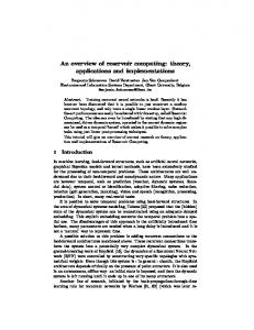
values of NT rain the difference between R(w) and Remp (w) could be non negligible. This means that in general a small error on the training set does not guarantee a small error on unseen examples (generalization error). A possible principled way to improve the generalization performances of a learning model consists in restricting its hypotheses space by limiting the complexity of the class of functions it can compute. One way to do so is provided by the VC-theory [181, 180]. This theory is based on a measure of the power of a class of functions, namely the VC dimension. By using a complexity measure like the VC dimension it is possible to provide an upper bound to the functional risk: R(w) ≤ Remp (w) + Φ(NT rain , V C(H), δ)

(2.3)

where V C(H) is the VC dimension of the hypotheses space H. Equation 2.3 holds for every NT rain > V C(H), with probability at least 1 − δ. The right hand side in (2.3) is also called the guaranteed risk and it is the sum of the empirical risk functional Remp (w) and the quantity Φ(NT , V C(H), δ), which is called the confidence term. If the number of available samples NT rain is fixed, as the VC dimension of H increases, the confidence term increases monotonically, whereas the empirical risk functional decreases monotonically. This is illustrated in Figure 2.1. The right choice is the hypothesis that minimizes the

Error

Bound on the generalization error

Confidence Term

Empirical Risk

0 VC dimension

Figure 2.1: The upper bound on the generalization error. guaranteed risk, i.e. something in the middle between a highly complex model and a too simple one. Minimizing the guaranteed risk is another inductive principle which is called the principle of structural risk minimization. It suggests to select a model which realizes the best trade-off between the minimization of the empirical error and the minimization of the complexity of the model.

28

2.1.3


Feed-forward Neural Networks

Feed-forward neural networks constitute a powerful class of learning machines which are able to deal with flat numerical data, facing supervised and unsupervised tasks. Neural networks are interesting for a number of reasons. In this context, we can appreciate the possibility of processing both numerical and categorical information, and computing in presence of noisy and partial data. Moreover, by adapting their free parameters based on known data samples, feed-forward neural networks are featured by universal approximation capabilities [38]. In addition to this, neural networks represent one of the most used and known class of ML models, successfully applied in many real-world applications. A deeper introduction to this class of learning machines can be found e.g. in [94, 28]. When computing with neural networks, the considered domains are numerical. In the following, RU and RY are used to denote the input and output spaces, respectively. From an architectural perspective, a feed-forward neural network is made up of simple units, also called neurons. Considering a single neuron, let x ∈ RU denote the input pattern, w ∈ RU a weight vector, and b ∈ R a bias. Then the output of the neuron is y = f (wT x + b) ∈ RY , where f is the activation function. The weight vector w and the bias b represent the free parameters of the neuron. Note that very often the bias is treated as an additional weight (with typically unitary associated input) and is therefore represented as an extra component within the weight vector w. The activation function determining the output of the neuron can be linear or non linear. Often the non-linear activation functions are of a sigmoidal type, such as the logistic function or the hyperbolic tangent function. Typical discrete output counterparts are the Heaviside or the sign threshold functions. Neural networks can be designed by composing units according to a specific topology. The most common topology provides for an organization of units in layers, where typically each unit in each layer is fed by the output of the previous layer and feeds the units in the following layer. Here we consider only feed-forward neural networks architectures, in which the signal flow is propagated from the input layer towards the output layer without feedback connections. In order to present an overview of the main characteristics of this class of models, let us focus on a particularly simple yet effective class of feed-forward neural networks, i.e. Multilayer Perceptrons (MLP). The architecture of a two-layered MLP is depicted in Figure 2.2, consisting in an NU -dimensional input layer, an hidden layer with NR units and an output layer with NY units. The function computed by the network is given by y(x) = fo (Wo fh (Wh x)) (2.4) where x ∈ RNU is the input pattern, y(x) ∈ RNY is the corresponding output computed by the MLP, Wh ∈ RNR ×NU and Wo ∈ RNY ×NR are the weight matrices (possibly including bias terms) for the connections from the input to the hidden and from the hidden to the output layers, respectively, and fh and fo denote the element-wise applied activation functions for hidden and output units, respectively. Note that fh (Wh x) ∈ RNR represents the output of the hidden layer. MLPs are mainly used to approach supervised tasks on flat domains, e.g. classification and regression from a real vector sub-space, and some kind of unsupervised tasks, such as dimensionality reduction. MLPs constitute a powerful class of learning machines, in fact a MLP with only one hidden layer can approximate any continuous function defined on a compact set, up to any arbitrary precision (e.g. see [38, 94]). Equation (2.4) describes the hypotheses class associated to MLPs. The particular hypothesis is selected by choosing the weight values

29


Wh

Wo

.. .

x

.. .

y

.. .

Input Layer

Hidden Layer

Output Layer

Figure 2.2: Architecture of an MLP with two layers.

in the weight matrices, i.e. the elements of matrices Wh and Wo , which represent the free parameters of the model. Assuming a supervised learning setting and given the training T rain set Ttrain = {(x(i), ytarget (i))}N , the learning algorithm should tune the free parami=1 eters of the model in order to reduce a discrepancy measure between the actual output of the network and the desired one, for each example in the training set. To this aim, the most known and used learning algorithm for MLPs is the Back-propagation Algorithm, which is an iterative algorithm implementing an unconstrained minimization of an averaged squared error measure, based on a gradient descent technique. The error (loss) function to be minimized is Emse =

1 NT rain

NX T rain

kytarget (i) − y(x(i))k22 .

(2.5)

i=1

Note that equation 2.5 corresponds to the definition of the empirical risk in equation 2.2, by using a quadratic loss function. Once the actual output of the network has been computed for each input pattern in the training set, the averaged squared error is computed using equation 2.5, and the weights can be adjusted in the direction of the gradient descent: (l)

∆wji ∝ − (l)

∂Emse (l)

∂wji

(2.6) (l)

where wji denotes the weight on i-th connection for neuron j in layer l, and ∂Emse /∂wji is the gradient of the error with respect to the weight. The rule of equation 2.6 is applied until the error measure Emse goes through a minimum. The error surface is typically characterized by local minima, so the solution found by the Back-propagation Algorithm is in general a suboptimal solution. Slow convergence is another known drawback of this gradient descent method. Other training algorithms have been designed for multilayer perceptrons, such as [48, 18, 128], just to cite a few. They try to overcome typical gradient descent disadvantages by using other optimization methods, e.g. second-order information or genetic algorithms.

30


Another relevant issue about feed-forward neural networks concerns the optimum architectural design of MLPs. One solution to this problem is given by the Cascade Correlation algorithm [47], which follows a constructive approach such that hidden neurons are progressively added to the network. Simply put, Cascade Correlation initializes a minimal network with just an input layer and an output layer, and then adds new units as the residual error of the network is too large. When the i-th hidden unit is added to the network, it is fully connected to the input layer and to the i − 1 already present hidden units. By using a gradient ascent method, the weights on these connections are trained to maximize the correlation between the output of the inserted unit and the residual error of the output units. After this phase, the trained connections are frozen, the i-th hidden neuron is fully connected to the output layer and all the connections pointing to the output layer are re-trained to minimize the training error. This approach is appealing for a number of reasons. Among all, it provides a way to make the network decide its own size and topology in a task dependent fashion, and secondly, in general, this algorithm learns faster than other training algorithms such as Back-propagation. Moreover, the Cascade Correlation approach has been extended to deal with structured data. Such extensions are described in Sections 2.2.4, 2.2.6 and 2.2.7.

2.1.4

Support Vector Machines and Kernel Methods

Support Vector Machines (SVMs) (e.g. [181, 180]) represent a class of linear machines implementing an approximation of the principle of structural risk minimization (Section 2.1.2). SVMs deal with flat numerical data and can be used to approach both classification and regression problems. To introduce the SVM model, let consider a binary clasT rain sification problem described by a set of training samples Ttrain = {(x(i), ytarget (i))}N , i=1 N U where for every i = 1, . . . , Ntrain , x(i) ∈ R and ytarget ∈ {−1, 1}. An SVM classifies an input pattern x by using a linear decision surface, whose equation is: wT x + b = 0.

(2.7)

which defines the hypotheses space: H = {y(x) = wT x + b|w ∈ RNU , b ∈ R}. A particular hypothesis is selected by choosing the values for the free parameters of the linear model, i.e. w ∈ RNU and b ∈ R. The free parameters of the SVM are adjusted by a learning algorithm in order to fit the training examples in Ttrain . If the points in Ttrain are linearly separable, then an infinite number of separating linear hyperplanes exist. The idea behind SVMs is to select the particular hyperplane which maximizes the separation margin between the different classes. This is graphically illustrated in Figure 2.3. Maximizing the separation margin can be shown to be equivalent to minimizing the norm of the weight vector w. This approached is principled in the Vapnik’s theorem [181, 180], which roughly states that the complexity of the class of linear separating hyperplanes is upper bounded by the squared norm of w. Thus, the complexity of the hypotheses space of an SVM can be controlled by controlling kwk22 . Thereby, training an SVM can be formulated in terms of a constrained optimization problem, consisting in minimizing an objective function Φ(w) = 1/2kwk22 under the condition of fitting the training set Ttrain , i.e. ytarget (i)(wT x(i) + b) ≥ 1 for every i = 1, . . . , Ntrain . If the classification problem is not linearly separable, then the objective function must be properly modified, in order to relax the strict fitting condition on the training set, through the use of a set of NT rain slack variables. The function to be minimized is

31


Separating Hyperplane

Support Vectors

separation margin

Figure 2.3: An example of linearly separable classification problem and optimal separation hyperplane.

Φ(w, ξ) = 1/2kwk22 +Ckξk22 , where ξ = [ξ1 , . . . , ξNT rain ]T is the vector comprising the slack variables and C > 0 is a positive user specified parameter, which acts as trade-off between the minimization of the complexity of the model and the minimization of the empirical risk. The minimization of Φ(w, ξ) is constrained by the conditions ytarget (i)(wT x(i)+b) ≥ 1 − ξi ∀i = 1, . . . , NT rain and ξi ≥ 0 ∀i = 1, . . . , NT rain . The optimization problem is solved using the method of Lagrangian multipliers, leading to the formulation of a Lagrangian function and then of a dual problem consisting in maximizing the function:

Q(α) =

NX T rain i=1

αi −

NT rain 1 X αi αj ytarget (i) ytarget (j) x(i)T x(j) 2

(2.8)

i,j=1

train with respect to the set of Lagrangian multipliers {αi }N i=1 , subject to the constraints PNT rain αi ytarget (i) = 0 and 0 ≤ αi ≤ C ∀i = 1, . . . , NT rain . Note that maximizing Q(α) i=1 is a problem that scales with the number of training samples. By solving the optimization problem, all the Lagrangian multipliers are forced to 0, except for those corresponding to particular training patterns called support vectors. In particular, a support vector (s) x(s) satisfies the condition ytarget (wT x(s) + b) = 1 − ξ (s) . In the case of linearly separable patterns, the support vectors are the closest training patterns to the separating hyperplane (see Figure 2.3). Once the maximization problem has been solved, the optimum solution for theP weight vector w can be calculated as a weighted sum of the support vectors, namely NT rain w = αi ytarget (i)x(i). Note that in this sum, only the Lagrangian multipliers i=1 corresponding to support vectors are non zero. The optimum bias b is computed in a

32


similar way. The decision surface can therefore be computed as NX T rain

αi ytarget (i) xTi x + b = 0.

(2.9)

i=1

Note that the previous equation 2.9, as well as the function Q in equation 2.8, depends on the training patterns only in terms of inner products of support vectors. Given a classification problem on the input space U , the Cover’s theorem about the separability of patterns [181, 37] roughly states that the probability that such classification problem is linearly separable is increased if it is non-linearly mapped into a higher dimensional feature space. This principle is used in SVMs, by resorting to a non linear function φ : U → X to map the problem from the original input space U into an higher dimensional feature space X . The optimization problem is then solved in the feature space, where the probability of linear separability is higher. The inner products in equations 2.8 and 2.9 can be applied in the feature space X without explicitly computing the mapping function φ, by resorting to a symmetric kernel function k : U × U → R. The kernel function k computes the inner product between its arguments in the feature space without explicitly considering the feature space itself (kernel trick ), i.e. for every x, x′ ∈ U : k(x, x′ ) = φ(x)T φ(x′ ).

(2.10)

By using a kernel function, equations 2.8 and 2.9 can be redefined such that each occurrence of an inner product is replaced by the application of the kernel function. A kernel function k can be considered as a similarity measure between its arguments, and therefore the classification problem can be intended as defined on pairwise comparisons between the input patterns. For a kernel function k to be a valid kernel, i.e. to effectively correspond to an inner product in some feature space, k must satisfy the Mercer’s condition [181], i.e. it has to be a positive definite kernel. Positive definite kernels have nice closure properties. For instance, they are closed under sum, multiplication by a scalar and product. Wrapping up, a classification problem is indirectly cast in an higher feature space nonlinearly by defining a valid kernel A dual problem consisting in maxPNTfunction. PNoptimization rain T rain imizing the function Q(α) = i=1 αi − 1/2 i,j=1 αi αj ytarget (i)ytarget (j)k(x(i), x(j)) T rain with respect to the variables {αi }N , and subject to certain constraints, is solved and n=1 P T rain the equation of the decisional surface is computed as N αi ytarget (i)k(x(i), x)+b = 0. i=1 The kernel function k must be defined a-priori and in a task specific fashion, moreover its proper design is of a central importance for the performance of the model. Two common classes of kernels are the polynomial kernel (i.e. k(x, x′ ) = (xT x′ + 1)p ) and the Gaussian kernel (i.e. k(x, x′ ) = exp(−(2σ 2 )−1 kx − x′ k22 ), which always yield valid kernels. Kernel functions can be used to extend the applicability of any linear learning method which exploits the inner product between input patterns to non linear problems. This can be done by simply substituting each occurrence of an inner product with the application of the kernel function. The family of learning models that resort to the use of a kernel function is known as kernel methods. An advantage of kernel methods is that it is often easier to define a similarity measure between the input patterns of a classification or regression problem, instead of projecting them into a feature space in which to solve the problem. Moreover, note that the feature space embedded into a valid kernel function


33

can have infinite dimensions. On the other hand, the main drawback involved by kernel methods is that each problem may require a specific a-priori definition of a suitable kernel function, which is fixed and not learned from the training data. Another critical aspect of kernel methods is related to the computational efficiency of the algorithm that computes the kernel function, whose design often requires particular care.

2.1.5

Nearest Neighbor

The Nearest Neighbor algorithm implements an instance-based approach for classification and regression tasks. Accordingly, the training phase simply consists in storing all the training data, while the output function is computed (based on local information) only when a new input pattern is presented. In this case the hypothesis is constructed at the test phase and locally to each input pattern. The underlying assumption is that the target output for an input pattern can be coherently computed to be more similar to the “closer” training samples in the metric space considered. T rain Suppose we have a training set Ttrain = {(x(i), ytarget (i))}N , where e.g. input i=1 N element are in an N -dimensional real sub-space, i.e. x(i) ∈ R ∀i = 1, . . . , NT rain , and a test sample x ∈ RN . The Nearest Neighbor algorithm associates to x the target output corresponding to the training sample n1 (x) ∈ {x(1), . . . , x(NT rain )} which is closer to x (using the Euclidean distance): y(x) = ytarget (n1 (x)).

(2.11)

A generalization of equation 2.11 is represented by the K-Nearest Neighbor algorithm, in which the K closest training input patterns to x, denoted as n1 (x), . . . , nK (x), are used to compute y(x). In particular, for classification tasks, y(x) can be computed as: y(x) = arg max y′

K X

δ(y′ , ytarget (ni (x))).

(2.12)

i=1

where δ(·, ·) is the Kronecker’s delta, and the classification of x is the most common classification among the K closest training input patterns to x. For regression tasks, e.g. when the output domain is a sub-set of R, the output for x can be computed as the average target output over the K training nearest neighbors of x, i.e. K 1 X y(x) = ytarget (ni (x)). K

(2.13)

i=1

The distance-weighted K-Nearest Neighbor algorithm is a common variant of the standard K-Nearest Neighbor, aiming to alleviate the effect of possible noise in the training input data. It consists in weighting the contributions of each nearest neighbor proportionally to the reciprocal of the distance from the test input pattern. In this way, closer neighbors have a stronger influence on the output, whilst very distant neighbors do not affect much the output computation. Given an input pattern x, let denote by wi the inverse square of the Euclidean distance between x and its i-th nearest neighbor ni (x), i.e. wi = 1/kx − ni (x)k22 . For classification tasks, equation 2.12 is modified according to: y(x) = arg max y′

K X i=1

wi δ(y′ , ytarget (ni (x))).

(2.14)

34


while, for regression tasks, equation 2.13 is modified such that

y(x) =

K P

wi ytarget (ni (x))

i=1 K P

.

(2.15)

wi

i=1

2.1.6

Neural Gas

Neural Gas (NG) [136] is a clustering algorithm. In general, clustering algorithms are used to partition a set of observations in groups, such that more similar observations tend to fall within the same group. Considering a set S ∈ RN , and a distance metric on S, denoted as d(·, ·), the goal consists in finding K prototype vectors (or cluster centroids) c1 , . . . , cK ∈ RN . Such vectors are used to encode the elements of S, such that each x ∈ S is represented by the winner prototype c(x) which is “closer” (in some sense) to x according to the metric d, i.e. typically d(x, c(x)) ≤ d(x, ci ) ∀i = 1, . . . , K. In this way the set S is partitioned in into K Voronoi cells: Si = {x ∈ S| d(x, ci ) ≤ d(x, cj ) ∀j = 1, . . . , K}

(2.16)

The prototype vectors are found by employing a training procedure aimed at minimizing T rain an error function E, given a training set Ttrain = {x(i) ∈ S}N . This often results i=1 in the definition of an iterative stochastic gradient descent algorithm consisting in the alternation of assignment and update steps. In the assignment step, each x ∈ Ttrain is associated to the winner prototype, while the update step adjusts the prototype vectors in order to decrease the error E. In the NG algorithm, the Euclidean distance is typically used ad metric on RN , and the update of prototypes is accomplished using a “soft-max” adaptation rule. According to this rule, after the presentation of each training sample x, all the K prototypes are modified. In particular, for a given training point x, a neighborhood-ranking r(x, c) ∈ {0, 1, . . . , K − 1} is assigned to each prototype (where the value 0 indicates the closer prototype and the value K − 1 indicates the most distant one). The adjustment for the i-th prototype is therefore computed as: ∆ci = ǫ hλ (r(x, ci )) (x − ci ) (2.17) where ǫ ∈ [0, 1] is a learning rate parameter. Typically hλ (r(x, ci )) = exp (−r(x, ci )/λ), where λ is a decay constant. In [136] it has been shown that the NG update rule in equation 2.17 actually implements a stochastic gradient decent on the error measure: EN G = (2 C(λ))

−1

K Z X

dN x P (x) hλ (r(x, ci )) (x − ci )2

(2.18)

i=1

P where C(λ) = K−1 k=0 hλ (k) is a normalization constant depending on λ and P (x) denotes the probability distribution of the elements in S. One the main advantages of the NG algorithm is its stability. Indeed, many clustering algorithms, including the popular K-means1 [125, 131], often provide a clustering which 1

Note that if λ → 0 in equation 2.17, then the K-means algorithm is obtained.


35

is strongly dependent on the initialization conditions (i.e. the initial values for the prototypes). By using the “soft-max” approach described above (equation 2.17), the NG algorithm usually converges quickly to stable solutions (independent of the prototype initialization). Interestingly, the name of the algorithm is due to the observation that the dynamics of the prototype vectors during the adaptation steps resemble the dynamics of gas particles diffusing in a space [136].

36

2.2


Neural Networks for Learning in Structured Domains

In this Section we give some basics of ML models for learning in structured domains, focusing the attention on neural networks for structures. We introduce the general framework for recursive processing structured data that is adopted in the rest of the thesis. The classes of Recurrent and Recursive Neural Networks, as well as the Reservoir Computing paradigm, are described within the introduced framework. Such framework is also used to review some of the most relevant models in the field of learning in structured domains, which represent related approaches to the Reservoir Computing framework for structured data described in Part III.

2.2.1

A General Framework for Processing Structured Domains

In this Section we introduce the framework adopted in this thesis for describing and characterizing data structures processing, especially by the means of neural networks. Structured Domains For structured data we mean some kind of information that can be described in terms of basic component entities and relations among them. In the following, by adopting a general perspective, as structured domain we will generally refer to a set of labeled graphs. A graph g in a set of graphs G is a couple g = (V (g), E(g)), where V (g) denotes the set of vertices of g and E(g) = {(u, v)|u, v ∈ V (g)} denotes the set of edges of g, representing a binary relation on V (g). The number of vertices of g is denoted by |V (g)|. With a slight abuse of notation, |V (g)| is also referred to as the size of g. In a directed graph g, the set of the edges is a subset of the product space V (g) × V (g), i.e. each edge has a direction. In this case, if (u, v) ∈ E(g) we say that (u, v) leaves (or is incident from) vertex u and enters (or is incident to) vertex v. We also say that u is a predecessor of v and that v is a successor of u. The set of all the predecessors of a vertex v ∈ V (g) is denoted by P(v) = {u ∈ V (g)| ∃(u, v) ∈ E(g)}, whereas the set of all the successors of v is denoted by S(v) = {u ∈ V (g)| ∃(v, u) ∈ E(g)}. In an undirected graph g, the set of edges consists of unordered pairs of vertices, i.e. no order is associated to the edges. In this case, if (u, v) ∈ E(g) we say that (u, v) is incident on the vertices u and v, and that u and v are vertices adjacent to each other. Given a graph g, a path of length l from vertex u to vertex v is a sequence of vertices < v0 , v1 , . . . , vl > where vi ∈ V (g) ∀i = 0, . . . , l, (vi , vi+1 ) ∈ E(g) ∀i = 0, . . . , l − 1, v0 = u and vl = v. If there exists a path from u to v, we say that v is reachable from u. In particular, if g is a directed graph, we say that u is an ancestor of v and v is a descendant of u. If g is an undirected graph and there exists a path from the vertex u to the vertex v, we say that u and v are connected. An undirected graph g is said to be connected whenever each pair of vertices in V (g) are connected. For a graph g, if every vertex in V (g) is reachable from the vertex v ∈ V (g), then we say that v is a supersource of g. Notice that for a graph g a supersource could not be defined, or more than one supersource could be present. For a directed graph g, the neighborhood of a vertex v ∈ V (g), denoted by N (v), is defined as theS union of the set of predecessors and of the set of successors of v, i.e. N (v) = P(v) S(v). If g is undirected, the neighborhood of vertex v ∈ V (g) consists in

37

2.2. NEURAL NETWORKS FOR LEARNING IN STRUCTURED DOMAINS

the set of the vertices which are adjacent to v, i.e. N (v) = {u ∈ V (g)|∃(u, v) ∈ E(g)}. In a directed positional graph g, for each vertex v ∈ V (g) a position is assigned to each predecessor and successor of v: the i-th predecessor of v is denoted by pi (v), whereas the i-th successor of v is represented as si (v). Analogously, in an undirected positional graph g, a position is assigned to each neighbor of v ∈ V (g). In this case, the i-th neighbor of v is denoted by Ni (v). Note that in case of a non positional graph g, for every vertex v ∈ V (g) an arbitrary enumeration of its successors and predecessors (if g is directed) or of its neighbors (if g is undirected) can be imposed (e.g. for the ease of notation). Note, however, that in this case any semantic interpretation of the position of the successors and predecessors (or of the neighbors) of a vertex is lost. A directed graph g is cyclic if there exists a path < v0 , . . . , vl > in g such that v0 = vl and l > 0. Analogously, an undirected graph g is said to be cyclic if there exists a path < v0 , . . . , vl > such that v0 = vl , l > 0 and the vertices in the path are all distinct. A graph g is said acyclic if it is not cyclic. For a directed graph g, the in-degree of a vertex v ∈ V (g) is the number of edges that enter v, i.e. the cardinality of P(v). Analogously, the out-degree of vertex v ∈ V (g) is the number of edges that leave v, i.e. the cardinality of S(v). The maximum in-degree and out-degree over the vertices in V (g) are referred to as the in-degree and the out-degree of graph g, respectively. The maximum in-degree and out-degree over the set G of considered graphs are denoted by kin and kout , respectively. For an undirected graph g, the degree of each vertex v ∈ V (g) is the number of vertices incident on it, i.e. the cardinality of N (v). The degree of g is the maximum degree over the set of its vertices V (g), whereas the maximum degree over a set of considered graphs G is denoted as k. When dealing with directed graphs, the term degree usually refers to the sum of the in-degree and the out-degree, i.e. k = kin + kout . Graphical representations of graphs are illustrated in Figure 2.4, which shows some examples of directed and undirected graphs. supersource

cycle

g1

g2

g3

Figure 2.4: Examples of graphs. In particular g1 is a directed acyclic graph (the arrow indicates the supersource), g2 is a directed cyclic graph and g3 is an undirected graph. In a labeled graph g, each vertex v ∈ V (g) has a numerical vectorial label associated to it. In general, assumed a vectorial label domain L, the label of a vertex v is usually denoted by l(v), while the set of directed graphs with maximum in-degree kin and maximum outdegree kout and vertices labels in L, is represented by L#(kin ,kout ) . For undirected graphs

38


with maximum degree k we use the analogous notation L#k . Whenever the degree is not specified, L# is used. The skeleton of a labeled graph g, denoted by skel(g), is the graph that is obtained by removing the label information associated to the vertices of g. Two graphs g1 = (V (g1 ), E(g1 )) and g2 = (V (g2 ), E(g2 )) are isomorphic if there exists a bijection f : V (g1 ) → V (g2 ) such that (u, v) ∈ E(g1 ) if and only if (f (u), f (v)) ∈ E(g2 ). Equivalently, g1 and g2 are isomorphic whenever their skeletons are the same, i.e. skel(g1 ) = skel(g2 ), while the labels associated to pairs of corresponding vertices might differ. Wrapping up all these definitions, we can consider some particularly interesting classes of data structures, e.g. sequences and trees, which can be viewed as special cases of labeled graphs. In the following definitions, we assume that vertex labels are in the domain L. A trivial graph is a graph with one vertex and no edges. As no any relation is defined among the components of a trivial graph, it can be recognized as an instance of an unstructured domain. Referring to the formalism introduced above, the set of trivial graphs can be also denoted by L#(0,0) . Examples of trivial graphs are fixed-size flat data representations, such as vectors and matrices. A sequence can be identified as a directed graph, with in-degree and out-degree equal to 1, catching a sequential relation among its vertices. Accordingly, a sequence can be considered as an instance in the structured domain L#(1,1) , which corresponds to the set of all finite length sequences over the alphabet L, i.e. L∗ . A sequence over L∗ is generally referred to using the symbol s(l), and the vertices of a sequence are usually called elements. The concatenation between two sequences s1 (l) and s2 (l) is denoted by s1 (l)· s2 (l). The binary relation represented by the set of the edges of a sequence s, is a total order over the set of the elements in s. In the following, we assume that if the edge (u, v) exists, then the element u follows the element v is the ordering. If a temporal dimension is involved (temporal sequences), a discrete time step t ∈ N is usually associated to each element of a sequence, and such elements can be indicated by referring to the value of the corresponding time step, e.g. s(l) = [l(1), . . . , l(n)] denotes a sequence on L∗ with length n. Note that in this case the temporal order is the opposite of the topological order of the structure (see Figure 2.5).

time . . .

l (1)

l (2)

. . .

l (t)

l (n−1)

l (n)

Figure 2.5: An example of a temporal sequence. A free tree is an undirected acyclic connected graph. In general, a tree is denoted by t and its vertices are also called nodes. The set of the nodes of a tree t is denoted by N (t). In particular, a rooted tree t is a free tree with one supersource node, called root and denoted by root(t). Rooted trees are particularly suitable data organizations for representing hierarchical relations among nodes. If a node n in a rooted tree has a


39

predecessor u, i.e. the edge (u, n) exists, then we say that u is the parent of n, and that n is a child of u. A k-ary rooted tree can be considered as an instance in the structured domain L#(1,k) , where k defines the out-degree of the structure. In this context, the root is the only vertex with null in-degree, the leaf nodes have a null out-degree, while internal nodes have positive in-degree and out-degree. The k children of a node n in a k-ary rooted tree are represented by ch1 (n), . . . , chk (n). Given a node n, by t(n) we denote the sub-tree rooted at n, i.e. the tree induced by the descendants of n and rooted at n. The depth of node n in the tree t is the length of the path from root(t) to n. The maximum over the depths of the nodes in t is called the height of t. In the following, we restrict our consideration to directed rooted trees. Thereby, when not differently specified, with the term tree we will refer to a directed rooted tree. In general, a k-ary tree is positional, i.e. for each node n it is possible to distinguish among the positions of its children. In a non positional tree, the children of each node n can be enumerated, but their positions cannot be distinguished. Figure 2.6 shows examples of binary trees, i.e. k-ary trees with k = 2. Note that sequences can be considered as special cases of trees, with in-degree and out-degree equal to 1.

root

leaf Figure 2.6: Examples of binary trees. Another relevant class of data structures is represented by directed acyclic graphs (DAGs) and by directed positional acyclic graphs (DPAGs). Interestingly, DPAGs represent a generalization of positional trees, in which each node is allowed to have more than one parent (see e.g. the graph g1 in Figure 2.4). Transductions on Structured Domains We are interested in computing structural transductions [55], i.e. functions whose input and output domains are made up of graphs. The concept of structural transduction and the extension of the input domain are the ground to extend Reservoir Computing approaches for sequence (signal/series processes) to discrete hierarchical processing. Although new in the context of Reservoir Computing, the description in this Section is rooted in the previous framework for RecNN approaches for both supervised [169, 55, 86, 138] and unsupervised learning [87]. In the following, for the sake of simplicity, we will refer to the notation established for undirected graphs. Note, however, that the notions introduced can be easily re-stated for

40


the case of directed graphs. A structural transduction T is a function that maps an input graph domain U # into an output graph domain Y # : T : U# → Y# (2.19) where U and Y respectively denote the input and output label spaces, and the output graph corresponding to g ∈ U # is usually denoted by y(g). Structural transductions can be qualified in different ways. We say that T is a structureto-structure transduction2 if it maps input graphs into isomorphic output graphs, i.e. for every g ∈ U # it holds that skel(g) = skel(y(g)). Equivalently, T associates an output vertex in correspondence of each input vertex. Note that when a specific class of structures is under consideration this can be explicitly expressed. We can therefore have graph-tograph, tree-to-tree and sequence-to-sequence transductions3 . T is a structure-to-element transduction4 whenever it maps input graphs into flat (vectorial) outputs, i.e. for every g ∈ U # only one output element is produced. Equivalently, the output domain of T is actually a trivially structured (vectorial) domain, i.e. T : U # → Y. Also in this case, the class of structures can be made explicit, considering e.g. graph-to-element transductions, tree-to-element transductions or sequence-to-element transductions. Whenever the structured input domain is made up of hierarchical structures, e.g. trees or DPAGs, we say that the structural transduction T is causal if the function computed in correspondence of a particular vertex v depends only on v itself and on the descendants of v. A structural transduction T is adaptive if it learned from observed data, whereas it is fixed if it is a-priori defined. T is a stationary transduction if the function it computes does not depend on the particular vertex to which it is applied. Note that if T is non-stationary, the output computed in correspondence of each vertex in the input graph could be obtained by a different function. In the following, we always assume stationarity of the considered transductions, which has a specific relevant meaning in the case of learning in structured domains (as described in Section 2.2.4). A structural transduction T can be usefully decomposed as T : Tout ◦Tenc , where Tenc is the encoding transduction and Tout is the output transduction. The encoding transduction Tenc : U # → X #

(2.20)

maps an input graph g ∈ U # into a graph structured feature isomorphic to g, i.e. Tenc (g) ∈ X # , where X denotes the feature label space. In the following, we use also the symbol x(g) to denote the output of the encoding transduction Tenc applied to g. In addition, X is also referred to as a state label space, and x(g) as the structured state associated to g. The output transduction Tout : X # → Y # (2.21) 2

The notion of struture-to-structure transduction has been referred to in literature also as input-output isomorphic transduction (e.g. [86]) and as node-focused transduction (e.g. [160]). 3 The notion of sequence-to-sequence transduction has been referred to in literature also as synchronous sequential transduction (see [55]). 4 The notion of struture-to-element transduction has been referred to in literature also as supersource transduction e.g. in [86], with particular regard to hierarchical data processing, and as graph-focused transduction e.g. in [160].

41


maps the structured state representation of the input graph g, i.e. x(g), into the structured output representation Tout (g) = y(g) ∈ Y # . In order to realize structure-to-element transductions, we preliminarily resort to a state mapping function χ : X# → X

(2.22)

that maps a structured state x(g) into a flat (vectorial) state representation χ(x(g)). In this case, T = Tout ◦ χ ◦ Tenc . Figures 2.7 and 2.8 illustrate schematically through examples the computation of structureto-structure and structure-to-element transductions. In both cases, through the encoding transduction Tenc (equation 2.20), the input graph g is mapped into the graph structured feature representation x(g) isomorphic to g, i.e. x(g) has the same skeleton of g, but the labels attached to the vertices of x(g) are in the state space X (this point is represented by using different colors for the vertices of the graphs in Figures 2.7 and 2.8). Then, in the case of structure-to-structure transductions (Figure 2.7) the structured output y(g) is obtained by directly applying the output transduction Tout (equation 2.21) to x(g). Note that in this case y(g) is isomorphic to both g and x(g). In the case of structure-to-element transductions (Figure 2.8), the structured state x(g) is first mapped by the state mapping function χ (equation 2.22) into a fixed-size vectorial state representation, i.e. χ(x(g)). Then the output transduction is applied to χ(x(g)) in order to obtain the output vector y(g).

T enc

T out x(g )

g

y(g )

Figure 2.7: A structure-to-structure transduction.

χ

T enc g

x(g )

T out χ (x(g ))

y(g )

Figure 2.8: A structure-to-element transduction. In the context of a supervised learning paradigm, for a task involving a structure-tostructure transduction, a training set can be described as Ttrain = {(gi , ytarget (gi ))| gi ∈ U # , ytarget (gi ) ∈ Y # ∀i = 1, . . . , Ntrain }, where gi and ytarget (gi ) respectively denote the i-th input and the i-th target output structure, and Ntrain is the number of samples in the

42


dataset. For task involving structure-to-element transductions, the previous notation is straightforwardly modified such that the target output associated to each input structure is indeed a single flat element, i.e. Ttrain = {(gi , ytarget (gi ))| gi ∈ U # , ytarget (gi ) ∈ Y ∀i = 1, . . . , Ntrain }. In this concern, note that regression or classification tasks on structures can be considered as special cases in which the target output associated to each gi is a real number, i.e. y(gi ) ∈ R, or a vector encoding a class label, e.g. for binary classification y(gi ) ∈ {−1, +1}. In the following sub-sections, we discuss how structural transductions can be computed in a recursive fashion. Recursive approaches, indeed, turn out to be particularly suitable for processing such transductions by the means of neural networks models.


2.2.2

43

Recursive Processing of Transductions on Sequences

Within the framework established in Section 2.2.1, here we describe a recursive approach which is typically considered when processing causal and stationary transductions on sequence domains e.g. by using Recurrent Neural Networks. In the following, we use the symbol s(u) to denote an input sequence in U ∗ . The sequence s(u) can be either an empty sequence, denoted by s(u) = [], or a sequence of length n > 0, i.e. s(u) = [u(1), . . . , u(n)], in which case u(1) represents the oldest entry and u(n) is the most recent one. A transduction on sequence domains T : U ∗ → Y ∗ can be recursively computed by the means of locally applied encoding and output functions. In particular, the encoding transduction Tenc : U ∗ → X ∗ is computed by resorting to a local encoding function τ that provides a state representation x(t) ∈ X in correspondence of each element of the input sequence u(t) ∈ U for t = 1, . . . , n: τ :U ×X →X (2.23) x(t) = τ (u(t), x(t − 1)) where an initial state x(0) ∈ X is defined. Note that equation 2.23 describes a state transition system on sequences. In this regard, the function τ can be viewed as a local state transition function. Corresponding to the extension to paths of the definition of state transition functions in finite automata [99], we can introduce an iterated version of τ , denoted by τˆ: τˆ : U ∗ × X → X

τˆ(s(u), x(0)) =

  x(0)

if s(u) = []

τ (u(n), τˆ([u(1), . . . , u(n − 1)], x(0))) if s(u) = [u(1), . . . , u(n)] (2.24) where τˆ(s(u), x(0)) is the state obtained by applying the state transition τ recursively to the input sequence s(u), starting from the initial state x(0). Function τˆ in equation 2.24 represents a global state transition function on input sequences. Given an initial state x(0) ∈ X , the computation of the encoding transduction Tenc (s(u)) can be therefore obtained by applying the global state transition function τˆ to s(u) and x(0), i.e. τˆ(s(u), x(0)). In the following, the process consisting in the computation of the encoding transduction Tenc is also referred to as the encoding process. The output transduction Tout : X ∗ → Y ∗ is computed by resorting to a locally applied output function gout : gout : X → Y (2.25) y(t) = gout (x(t)) 

where y(t) ∈ Y is the element of the output sequence s(y) ∈ Y ∗ computed in correspondence of the t-th element of the input. Note that equation 2.25 refers to the case of sequence-to-sequence transductions. For the case of sequence-to-element transductions, the output sequence degenerates into a single output element s(y) ∈ Y, obtained by applying the function gout only to the state corresponding to the last input element, i.e.

44


s(y) = y(n) = gout (x(n)), where n > 0 is the length of the input sequence. This is equivalent to using a state mapping function χ : X ∗ → X , such that for every s(x) of length n > 0 it holds that χ(s(x)) = x(n).

2.2.3

Recursive Processing of Transductions on Trees

In this sub-section we generalize the recursive approach described in the previous subsection for the case of tree domains processing. To this aim, we find useful to introduce a recursive definition of trees, as follows. A k-ary tree t ∈ U (1,k) can be defined as either the empty tree, denoted by nil, or as the root node n and the k sub-trees rooted in its children, denoted by n(t(ch1 (n)), . . . , t(chk (n))). Note that in this recursive definition, some of the k children of n could be absent (or missing), in which case the corresponding sub-trees are empty. The suffix of height h ≥ 0 of a tree t, indicated as Sh (t), is the tree obtained from t by removing every node whose depth is greater than h:  nil if h = 0 or t = nil    Sh (t) = if h > 0 and t = n(t(ch1 (n)), . . . ,    n(Sh−1 (t(ch1 (n))), . . . , Sh−1 (t(chk (n)))) t(chk (n))) (2.26) Analogously to the case described for the recursive processing of sequences, causal and stationary structural transductions on k-ary tree domains, such as T : U #(1,k) → Y #(1,k) , can be computed by resorting to local node-wise applied encoding and output functions, where u(n) ∈ U , x(n) ∈ X and y(n) ∈ Y are used do denote input, state and output labels for the node n, respectively. The encoding transduction Tenc : U #(1,k) → X #(1,k) , can be computed by using to a node-wise encoding function τ : τ : U × Xk → X (2.27) x(n) = τ (u(n), x(ch1 (n)), . . . , x(chk (n))) where x(n) is the state representation computed for node n and x(ch1 (n)), . . . , x(chk (n)) are the states associated to the children of n. Equation 2.27 describes the relation between the state corresponding to a node n and the states corresponding to its children. As such, equation 2.27 defines a state transition system on trees and τ can be viewed as a local state transition function. Note that if one of the children of n is absent, then a nil state, denoted by x(nil), is used for it (analogously to the initial state x(0) used for sequence processing). The node-wise encoding function τ of equation 2.27 induces a recursive function on trees, denoted by τˆ: τˆ : U #(1,k) × X → X

τˆ(t, x(nil)) =

 x(nil)   

if t = nil

   τ (u(n), τˆ(t(ch1 (n)), x(nil)), . . . , τˆ(t(chk (n)), x(nil))))

if t = n(t(ch1 (n)), . . . , t(chk (n)))

x(root(t)) = τˆ(t, x(nil)) (2.28)

45


where τˆ(t, x(nil)) is the state of the root of t, i.e. x(root(t)), given that the state for absent nodes is x(nil). Notice that the recursive definition of τˆ is given in equation 2.28 in analogy with the extension to paths of the definition of transition functions in finite automata [99]. Equation 2.28 describes the relation between the state of a node n and the states computed for the descendants of n, and can be viewed as a global state transition function. Thus, the computation of the structured feature representation corresponding to an input tree t, i.e. x(t) = Tenc (t), consists in the application of τˆ to t. This implies the computation of the state for each node n in t through the application of the node-wise encoding function τ according to a bottom-up visit of t (i.e. starting from the leaf nodes and ending in the root). According to the assumption of stationarity, function τ of equation 2.27 is applied in correspondence of every visited node n, taking as inputs the label of n, i.e. u(n), and the states already computed for the children of n, i.e. x(ch1 (n)), . . . , x(chk (n)). This bottomup recursive encoding process is shown in Figure 2.9 through two illustrative examples. Note that, given an input tree t, the output of the encoding process x(t) = Tenc (t), can d

d c

c b

b a

a

τ τ τ τ

e

e d a

c

d

b

a

τ

x(nil ) x(nil )

x(nil )

τ

τ

c b

τ

τ

x(nil ) x(nil )

x(nil ) x(nil )

(b)

(a)

Figure 2.9: Bottom-up recursive encoding process on trees. Example (a) shows the process of visit for the special case of sequential input (i.e. k = 1), while example (b) shows the same process for the case of binary trees (i.e. k = 2). be considered as a tree which is isomorphic to t (according to the definition provided in Section 2.2.1) by construction. Indeed, while computing x(t), the recursive encoding process preserves the skeleton of t, while for each node n ∈ N (x(t)) the corresponding label x(n) is the state vector computed by the local state transition function τ . Note that this characterization is inherited from the concept of synchronism in sequence processing, generalized for the case of hierarchical structures processing (see [55, 86]). The output transduction Tout is then used to map the structured state representation of an input tree into its corresponding output. For tree-to-tree transductions T , the output transduction Tout is also tree-to-tree, i.e. Tout : X #(1,k) → Y #(1,k) . Given an input tree t ∈ U #(1,k) and its structured state x(t) ∈ X #(1,k) obtained through the recursive encoding, the structured output associated to t is y(t) = Tout (x(t)) ∈ Y #(1,k) . Tout can be computed by resorting to a node-wise output function gout : gout : X → Y (2.29) y(n) = gout (x(n))

46


where y(n) ∈ Y is the (unstructured) output associated to node n. In this case y(t) is computed by applying function gout to every node of t. For the case of tree-to-element transductions, the state mapping function χ : X #(1,k) → X is used to map the structured state x(t) into a flat feature representation χ(x(t)), which is representative for the whole input tree. The unstructured fixed-size output y(t) ∈ Y is then computed by applying the node-wise output function gout of equation 2.29 only to the output of the state mapping function, i.e. y(t) = gout (χ(x(t))).

In the following, as label domains of interest, with particular regard to structure domain processing using neural networks, we consider the NU -dimensional real input space RNU , the NR -dimensional real state space RNR and the NY -dimensional real output space RNY . Accordingly, the input, state and output structure domains are represented by (RNU )# , (RNR )# and (RNY )# respectively.

2.2.4

Recurrent Neural Networks

Recurrent Neural Networks (RNNs) [121, 178, 94] represent a class of neural network models that can compute causal, stationary and adaptive transductions on sequence domains. RNNs are obtained by implementing the local encoding and output functions in equations 2.23 and 2.25 (Section 2.2.2) by the means of neural networks. In the simplest architectural setting, an RNN is composed of an NU -dimensional input layer, an NR -dimensional recurrent hidden layer and an NY -dimensional feed-forward output layer. The local encoding function is computed by the hidden layer, while the output function is computed by the output layer. More specifically, the hidden layer computes the recurrent state transition function τ : RNU × RNR → RNR , as follows: ˆ x(t) = f (Win u(t) + Wx(t − 1))

(2.30)

where u(t) is the input for the network at pass t and x(t) is the state of the network, i.e. the output of the hidden units, at pass t. The matrix Win ∈ RNR ×NU contains the weights on the connections from the input to the hidden layer (and possibly a bias term). The element-wise applied activation function f in equation 2.30 is usually a non-linearity of a sigmoidal type, such as the logistic function or the hyperbolic tangent. The matrix ˆ ∈ RNR ×NR contains the recurrent weights for the feedback connections around the W hidden units. The output layer computes the output function gout : RNR → RNY , as follows: y(t) = fout (Wout x(t)) (2.31) where y(t) is the output of the network at pass t and Wout ∈ RNY ×NR contains the weights of the connections from the hidden units to the output units (and possibly a bias term). The function fout in equation 2.31 is the element-wise applied activation function for the output units, and can be both a linear or a non-linear function. In a RNN, the encoding process is carried out by unfolding the hidden layer architecture on the input sequence. For sequence-to-sequence transductions the output layer computes the output element at each pass, i.e. equation 2.31 is applied to every state x(t) obtained by the hidden layer while the network is driven by the input sequence. For the case of sequence-to-element transductions, equation 2.31 is applied only to the state computed by


47

the hidden layer of the network in correspondence of the last element of the driving input sequence. The Cascade Correlation approach can be extended to RNNs as well [49]. In this case, when a new hidden unit is added to the network architecture, it receives input connections from the input layer and the state information coming from the already frozen hidden neurons. In a standard RNN, the parameters of both the encoding function and the output ˆ and function are learned from examples, i.e. the weight values in the matrices Win , W Wout are adjusted by a training algorithm. Concerning this aspect, it is worth to emphasize that the class of RNNs is theoretically very powerful, indeed through training RNNs are characterized by universal computational properties (e.g. [167]). A number of training algorithms for RNN models have been proposed in literature, sharing the basic idea of implementing a gradient descent method to back-propagate the error as in the Back-propagation algorithm for feed-forward neural networks. Among all, the most known are the Back-propagation Through Time (BPTT) algorithm [191] which is typically applied off-line, and the Real-Time Recurrent Learning (RTRL) algorithm [192], which is used on-line. However, training algorithms for RNNs involve some known drawbacks (e.g. [89, 127]). First, as other gradient descent methods they are characterized by high computational training costs and slow convergence. Second, as the error function considered by such algorithms is in general a non-convex function, they can get trapped in local minima of the error surface. Third, learning long term dependencies by gradient descending is known to be a difficult problem. This last point is also known as the problem of the vanishing gradient [121, 19], i.e. for long temporal dependencies the gradient information vanishes as it is back-propagated through time and the weights of the RNN are not correctly adjusted to properly take into account inputs in a far past. Overall, designing efficient yet effective training algorithms for RNNs still represents an open research issue (e.g. see [7, 168]). An interesting characterization of RNNs is provided by the study of the properties of the state dynamics in the early stages of training. Indeed, typically used initializations of network weights with small values (thus with contractive state dynamics) result in a architectural bias of the model ([90, 176, 175, 177]). Indeed RNNs initialized with contractive state transition functions have been proved to discriminate among different (recent) input histories even prior to learning ([90, 175]), according to a Markovian organization of the state dynamics. A recently proposed efficient alternative approach to RNN modeling is represented by the Reservoir Computing paradigm, which described in the next Section.

2.2.5

Reservoir Computing and Echo State Networks

Reservoir Computing (RC) (e.g. [184, 127]) is a denomination for a RNN modeling paradigm based on a conceptual and practical separation between a recurrent dynamical part (the reservoir ) and a simple non-recurrent output tool (the readout). Typically, the reservoir is implemented by a large (high dimensional) and random layer of sparsely connected recurrent hidden units, which is initialized according to some criterion and then left untrained. The readout is implemented through a layer of (typically) linear units and is adapted by using a simple and efficient training algorithm for feed-forward networks. RC is also claimed to have a strong biological plausibility. Indeed several relationships have

48


been discovered between the properties of animal brains and reservoir networks. Examples of these relationships can be found in [148, 43, 44, 194, 73]. Moreover, it is interesting to observe that some basic ideas of reservoir computation can be also viewed as an extension to the sequence processing case of the work on sparse distributed memories described in [114]. Reservoir networks implement causal, stationary and partially adaptive sequence transductions in which the encoding function (the state transition function) is realized by a fixed dynamical reservoir, and the output function is realized by the adaptive readout. The key observation about reservoirs is that as long as they satisfy some very easy-tocheck properties, they are able to discriminate among different input histories even in the absence of training. In this way it is possible to restrict the training just to a simple recurrent-free linear readout. This eliminates the recurrent dependencies in the weight adjusting process and leads to a very efficient RNN design. RC comprises several classes of RNN models, including the popular Echo State Networks (ESNs) ([103, 108]), Liquid State Machines (LSMs) (e.g. [129]) and other approaches such as BackPropagation Decorrelation (BPDC) ([171, 172]) and Evolino (e.g. [163]). In this thesis we focus on the ESN model.

An Echo State Network (ESN) ([103, 104, 105, 108]) is a RNN consisting in an input layer of NU units, a large number of NR sparsely connected recurrent hidden units (the reservoir ) and an output layer of NY typically linear and non-recurrent units (the readout). As in standard RNNs, the recurrent hidden layer of the architecture, i.e. the reservoir, implements the local encoding function τ of equation 2.23, while the feed-forward output layer, i.e. the readout, implements the local output function gout of equation 2.25. The basic equations 5 describing the computation carried out by an ESN are similar to the equations 2.30 and 2.31: ˆ x(t) = τ (u(t), x(t − 1)) = f (Win u(t) + Wx(t − 1)) (2.32) y(t) = gout (x(t)) = Wout x(t) where Win ∈ RNR ×NU is the input-to-reservoir weight matrix (possibly including a bias ˆ ∈ RNR ×NR is the recurrent reservoir weight matrix and Wout ∈ RNY ×NR is term), W the reservoir-to-output weight matrix (possibly including a bias term). Equation 2.32 also describes the basic ESN architecture (illustrated in Figure 2.10), which hereafter is referred to as the standard ESN. The hyperbolic tangent is typically used as activation function of reservoir units (i.e. f ≡ tanh), while the output of the network is a linear combination of the reservoir output. Referring to the framework of Section 2.2.1, we can say that ESNs compute partially-adaptive sequence transductions in which the encoding function is fixed and the output function is adapted from training data. This means that ˆ are fixed and only Wout is adapted. Not every choice of Win and W ˆ leads Win and W to a valid ESN. In a sense, the state of the network should be an echo of its input history (i.e. the reservoir dynamics must asymptotically depend only on the driving input signal). 5 Common variants to the proposed basic equations can be found in [103], in which connections from the input layer to the readout are allowed as well as feedback connections from the readout to the reservoir.

49


^

W u( t )

.. .

Wout

Win

.. .

y (t )

x (t ) Input

Reservoir

Readout

Figure 2.10: The architecture of an ESN. Echo State Property A valid ESN satisfies the so called Echo State Property (ESP) [103]. This says that the state in which the network is after being driven by a long input sequence does only depend on the input sequence itself. The dependence on the initial state of the network is progressively lost, as the length of the input sequence goes to infinity. Equivalently, the current state x(n) of the network is a function of its past input history independently of initial state values. In formulas, the ESP may be expressed as follows: ∀s(u) = [u(1), . . . , u(n)] ∈ (RNU )n input sequence of length n, ∀x, x′ ∈ RNR :

(2.33)

kˆ τ (s(u), x) − τˆ(s(u), x′ )k → 0 as n → ∞ which means that the distance between the states in which the network is driven by an input sequence of length n approaches zero (for any choice of the initial states) as n goes to infinity. In [103] two conditions have been provided as necessary and sufficient, respectively, for an ESN (with tanh as activation function) having echo states. The necessary condition is that the spectral radius (i.e. the largest eigenvalue in absolute value) of the ˆ is less than one reservoir recurrent weight matrix W ˆ 0, two input prefixes s(v), s(w) ∈ (RNU )∗ , common input suffix of length n [u(1), . . . , u(n)] and couple of initial states x, x′ ∈ RNR , the distance between the states computed by the reservoir for the two sequences s(v)· [u(1), . . . , u(n)] and s(w)· [u(1), . . . , u(n)], with initial states x and x′ respectively, is upper bounded by a factor proportional to C n :

kˆ τ (s(v)· [u(1), . . . , u(n)], x) − τˆ(s(w)· [u(1), . . . , u(n)], x′ )k ≤ C n diam

(3.4)

68

CHAPTER 3. MARKOVIAN AND ARCHITECTURAL FACTORS OF ESN DYNAMICS

In fact, kˆ τ (s(v)· [u(1), . . . , u(n)], x) − τˆ(s(w)· [u(1), . . . , u(n)], x′ )k ≤ Ckˆ τ (s(v)· [u(1), . . . , u(n − 1)], x) − τˆ(s(w)· [u(1), . . . , u(n − 1)], x′ )k ≤ ...

(3.5)

≤ C n kˆ τ (s(v), x) − τˆ(s(w), x′ )k ≤ C n diam The Markovian characterization of ESNs implies the fact that older input symbols have an exponentially decreasing influence on the reservoir state. Therefore the distance between the states corresponding to input sequences which differ only before a common suffix of length n, is anyhow bounded by a term which exponentially decreases with n. In this way, the reservoir of an ESN is able to differentiate different input sequences in a Markovian suffix-based way even in the absence of learning of the recurrent state transition function. Such state space organization makes the model more suitable for tasks for which more similar targets are associated to input sequences sharing longer suffixes. This is graphically illustrated in Figure 3.1, showing different (symbolic) input sequences and corresponding states computed by a model respecting the suffix-based Markovian organized dynamics. In the simplified example of Figure 3.1, the states corresponding to different input sequences cluster together in a suffix-based fashion. The two sequences ”cbaaba” and ”baaaba”, sharing the suffix ”aaba”, are mapped into close states, whereas the state corresponding to ”cbbaab” is quite distant. Thereby, the readout naturally performs better if the task at hand requires to associate similar outputs to ”cbaaba” and ”baaaba” and a different one to ”cbbaab”. On the contrary, the model is less appropriate whenever the task requires similar outputs for ”cbaaba” and ”cbbaab” and a different one for ”baaaba”. To concretely show the effect of the Markovian factor on possible classes of tasks, in Section 3.5.1 we design two ad-hoc target functions that match and un-match, respectively, the Markovian characterization of state dynamics, thereby characterizing suitable (easy) and un-suitable (hard) tasks for the ESN approach. When we move to a more realistic setting of finite precision computations, the differences between reservoir states corresponding to input sequences with long common suffixes can be appreciated up to a maximum suffix length, depending on both the precision of computation and the degree of contractivity of the state transition function. Input sequences with differences occurring only before a suffix of the maximum length are mapped into the same state. Thereby, finiteness of memory in reservoir computation arises, which is also supported by the results on the ”fading memory” property of reservoirs ([103]) and has been investigated in the context of the short-term memory capacity of ESNs (e.g. [105, 23]). However, note that even within the framework of finite memory computation, the Markovian nature of the reservoir space organization of equation 3.4, continues to hold. Such characterization determines the decreasing relative influence on the network state due to older elements of the input sequence and, differently from what is usual in ESN literature, shifts the focus on the properties of input sequences and corresponding targets, independently of the features of reservoirs and readouts.

69

3.3. MARKOVIAN FACTOR OF ESNS

common suffix

cbaaba

common suffix

cbbaab

baaaba

NR

State Space IR

bbbaab

Influence on the state Figure 3.1: Graphical illustration of the Markovian nature of reservoir state space organization. Input sequences with similar suffix drive the model into close points in the reservoir state space RNR (see equation 3.4).

Hence, independently of the architectural design, ESNs with contractive state dynamics are characterized by the Markovian factor. In [90] it has been shown that the architecture of RNNs with small recurrent weights is biased toward Markovian models. Therefore, during training standard RNNs initially explore regions of the state space within such Markovian characterization, before possibly moving towards more complex state dynamics [90]. In this concern, note that in the case of ESNs, the recurrent reservoir weights are never trained after the contractive initialization (see Sections 2.2.5 and 3.2). Thereby, for ESNs, Markovianity of the state space organization (as described in [90]) represents a strict and fixed characterization of the model [62]. However, note that the question whether contractivity of state transition functions is strictly necessary for the ESP to hold still represents an open problem, and in general the Markovian characterization is assured only when the contractivity is enforced. Therefore, in this Chapter the contraction coefficient σ is used to scale the reservoir weight matrix and to control the Markovian factor, with a smaller σ corresponding to a more prominent Markovianity of reservoir dynamics. There is another interesting question arising from the observation that the class of contractive ESNs is equivalent to the class of models with state space organization of Markovian nature. As contractivity seems to be the ruling characteristic of reservoirs, then one could expect that even a smaller contractive reservoir, or a contractive reservoir of neurons with any possible architecture of connectivity (e.g. only self recurrent connections) would perform well on suitable tasks just as standard ESNs would do. If this intuition were true, then even a single-unit reservoir (even a linear one) could be used to solve any such task as long as it is characterized by a contractive state dynamics. However, several works have reported that larger reservoirs of neurons have better predictive performances than smaller ones on different non-linear tasks (e.g. see [184]). Increasing the dimensionality of reservoirs seems to be the simplest way to get better performances. Moreover, as pointed out in [150], different reservoir instances, obtained with the same scaling settings of the

70


recurrent weight matrix, may result in different performances on the same task. Our investigation about the key architectural factors which may improve large reservoirs performance stems from these observations. Accordingly, several architectural variants of the standard ESN model are introduced in Section 3.4.

3.4

Architectural Factors of ESN Design

Even though reservoirs dynamics are governed by the Markovian factor, there still are several other factors, related to the architectural design, which might influence the richness of the Markovian dynamics and thus the performance of ESNs. Indeed ESNs with the same contractive coefficient but different topologies can lead to different results on the same task. At the same time, the richness of the dynamics is related to the growth of the number of units (reservoir dimensionality). It is therefore interesting to investigate the factors determining the differentiation among the units. We identified four architectural factors which may have an impact on ESNs performance, namely: input variability, multiple time-scale dynamics, non-linear interactions among units and regression in an augmented feature space. Each factor is described more extensively in the following: Input Variability. This refers to the possibility for different reservoir units of looking at each element of the input sequence under different points of view. The configuration without input variability is obtained by fixing the same values of the input weights for all the reservoir units. Input variability is implemented through a random initialization of the input-to-reservoir weight matrix Win with different values among units. Multiple Time-Scale Dynamics. This refers to the possibility for the reservoir units to behave as dynamical systems with different time-scale dynamics. Supporting multiple time-scales is equivalent to a reservoir having individual neurons with different contractive dynamics. We implement this possibility by controlling the reservoir ˆ As said in Section 3.2, the contractive dynamics of recurrent weight matrix W. the reservoir is governed by the contraction coefficient of the state transition funcˆ 2 . However, individual reservoir tion, which in the Euclidean norm is σ = kWk ˆ is arranged in a proper neurons may exhibit different contractive dynamics if W ˆ way. In particular, we study the case in which W is a diagonal matrix. In this case σ = maxi=1,...,NR σi , where σi is the contraction coefficient of each single unit i. This situation is equivalent to a RNN with self-recurrent connections only in the hidden layer. If different self-recurrent weights are used, then each neuron is able to show different contractive dynamics while being driven by the same input sequence. The Markovian behavior of the ESN does not only depend on the global value of σ but on the whole set of dynamics determined by the single values σi , ∀i = 1, . . . , NR . We conjecture that this architectural factor is crucial to achieve a rich dynamics of the global transition function corresponding to good predictive performance. Non-linear Interactions among Units. This factor refers to the presence of non-linear ˆ interactions among unit activations in a reservoir. It is implemented by using a W matrix with non-zero extra-diagonal values, i.e. the reservoir units are mutually connected. Note that using mutually and self-recurrent connectivity (including also

71

3.4. ARCHITECTURAL FACTORS OF ESN DESIGN

non-zero diagonal values), the different units dynamics due to the multiple time-scale factor are enriched by a non-linear recurrent combination of the dynamics of each unit. We consider both the cases of a dense recurrent matrix (fully connected reservoir) and a sparse recurrent matrix (sparsely connected reservoir). Note that since the very first work on ESNs ([103]) this architectural factor is one of those that are claimed to be responsible for producing “rich” reservoir dynamics, and thus good predictive performance. We propose to study this point in comparison to the other three identified and to show how it really influences the performance of reservoirs. Moreover, through a comparison between the sparsely and the fully connected architectures we intend to investigate if a full connectivity among neurons is actually needed to observe an influence of the non-linear interactions among units factor or if a small number of recurrent connections among neurons is sufficient. Regression in an Augmented Feature Space This factor refers to the influence that having a high dimensional non-linear reservoir may have in the performance of an ESN. This last point has actually much to do with the readout part of ESNs. The conjecture here is that a linear readout might perform much better in a high dimensional (non-linear) feature state space. To assess and to measure the effect of this factor we introduce a particular reservoir variant which is called ϕ-ESN, in which a smaller number of recurrent reservoir units (thus a smaller number of network recurrent dynamics) is projected into an higher dimensional space by a non-linear mapping. This study should give some insight on how much of the goodness of ESN performance is due to a sufficient number of non-linear recurrent reservoir dynamics and how much of it is due to the possibility of discriminating input patterns in an augmented feature space (even with a linear readout). We propose to investigate how the identified factors influence the reservoir dynamics by studying architectural variants on the standard ESN model of equation 2.32 (see Figure 3.2). In particular, we consider the following architectures:

^

W u( t )

.. .

Wout

Win

.. .

y (t )

x (t ) Input

Reservoir

Readout

Figure 3.2: Basic architecture of an ESN with a number of NU = 3 input units, NR = 4 reservoir units and NY = 2 output units.

72


• ESN full . This corresponds to the standard ESN model described in Section 2.2.5, ˆ is characterized by full connectivity. where W ˆ is a sparse matrix. This distinction is useful to • ESN sparse. As above, but W study the effects of non-linear interactions among reservoir units even in presence of a very small number of such interactions. ˆ is a diagonal matrix4 • DESN3 . Stands for Diagonal Echo State Network, in which W whose diagonal entries w11 , w22 , . . . , wNR NR are all the same and such that |wii | = σ, ∀i = 1, 2, . . . , NR (see Figure 3.3). In this case σ is also equal to the spectral ˆ A particular case is when wii = σ, ∀i = 1, . . . , NR , that corresponds radius of W. to a reservoir having only positive self-recurrent connections: xi (t) = f (Win u(t) + σxi (t − 1)) ∀i = 1, 2, . . . , NR

(3.6)

The individual neurons of a DESN implement dynamical systems which are all governed by the same contractivity properties (the same Markovianity), but which may look at the same input sequence elements through different input weights depending on the presence or absence of input variability. In particular, in the absence of input variability, all neurons in the reservoir of a DESN are identical, and the dynamics of a DESN is the same as the dynamics of a single neuron reservoir. If input variability is added, every reservoir neuron may differentiate its dynamics and thus performance prediction is expected to be better in this latter case. • RDESN. Stands for Random Diagonal Echo State Network, which consists in a DESN with possibly different self-recurrent weights. If σ is the contraction coefficient ˆ are chosen according to a uniform of the reservoir, then the diagonal weights of W distribution in [−σ, σ] (see Figure 3.3). xi (t) = f (Win u(t) + wii xi (t − 1)) ∀i = 1, 2, . . . , NR

(3.7)

Also in this case the contractivity coefficient σ is equal to the spectral radius of ˆ The reservoir of a RDESN has NR self recurrent units, each of which is charW. acterized by contractive dynamics with different time-scales. This variant is mainly used to evaluate the influence that multiple time-scale dynamics might have on the model performance, in particular when compared with the DESN architecture. An architectural variant very similar to this one is known in the ESN literature as the Simple ESN (SESN) model by [53]. However, in the standard SESN setting the input weights to the reservoir are always fixed to 1.0 and the recurrent units are typically linear. • ϕ-ESN. This variant accounts for the last architectural factor, and its underlying idea can be traced back to the Cover’s theorem on the separability of patterns ([37]), 3

In literature the acronym DESN is also used to refer a different approach called Decoupled ESN model, introduced in [195] 4 Although the architectural differences between RNN models characterized by recurrent hidden units ˆ and with self-recurrent connections only (i.e. diagonal W) ˆ with full connectivity (i.e. fully connected W) are known to have an impact on the approximation capabilities of RNN networks [167, 121], here a diagonal reservoir architecture is introduced with the aim of evaluating, isolating and comparing the quantitative influence on the ESN performance due to the identified architectural factors.

73

3.4. ARCHITECTURAL FACTORS OF ESN DESIGN

^

W u( t )

.. .

Wout

Win

.. .

y (t )

x (t ) Input

Reservoir

Readout

Figure 3.3: Diagonal ESN architectures with a number of NU = 3 input units, NR = 4 reservoir units and NY = 2 output units. The same recurrent weight is shared by every reservoir unit for a DESN, while different recurrent weights are possible in an RDESN. stating that a pattern-classification problem is more likely to be linearly separable if it is projected non-linearly into a higher dimensional feature space. Accordingly, in ϕ-ESNs, the recurrent reservoir state space is projected into a higher dimensional feature space through a fixed non-linear random mapping. The state transition function τ computed by the reservoir of the ESN is decomposed into an encoding function τ ′ and a feature mapping ϕ: τ = ϕ ◦ τ′

(3.8)

where ϕ : RNR → RNϕ , and RNϕ is the new augmented reservoir state space. The reservoir is accordingly subdivided into a recurrent part, which implements τ ′ and acts as a standard dynamic reservoir, and a feed-forward (static) part, which implements the function ϕ: ϕ(x(n)) = fϕ (Wϕ x(n)) (3.9) where Wϕ ∈ RNϕ ×NR is the weight matrix (possibly including the bias) for the connections from the recurrent part to the feed-forward part of the reservoir. Wϕ is set with random values in a bounded range and is left untrained. In our settings, the hyperbolic tangent is used as non-linear activation function fϕ . As the feature state space is now RNϕ , the matrix Wout (of equation 2.32) is a NY × Nϕ + 1 matrix. Figure 3.4 illustrates the architecture of a ϕ-ESN. Note that the recurrent part of a ϕ-ESN may be arranged according to one of the previously described architectures. We can thus have ϕ-ESN full, ϕ-ESN sparse, ϕ-DESN and ϕ-RDESN. The non-linear map ϕ implemented by the feed-forward part of the reservoir increases the non-linearity (and the dimensionality) of the state mapping τ , thereby facilitating the readout for tasks that require high non-linear mapping capabilities in a richer space. Higher dimensionality of ϕ-ESN therefore comes with an augmented nonlinearity of reservoir dynamics. However, note that ϕ-ESN does not introduce in the architecture either non-linear recurrent dynamics (as the recurrent part is unchanged and the architecture is augmented with a static feed-forward layer) or a non-linear learner (as the adapted readout is still linear).

74


^

Wϕ

W u( t )

.. .

Wout

.. .

Win

.. .

y (t )

x (t )

Dynamic

Input

Reservoir

Static

Readout

Figure 3.4: Architecture of a ϕ-ESN, with a number of NU = 3 input units and NY = 2 output units. The dynamic part of the reservoir contains NR = 4 recurrent units, while the static part is implemented through a layer of Nϕ = 10 feed-forward units. The effects of improved non-linearity in reservoirs have more recently been addressed also in [26, 27], in which an RC architecture similar to ϕ-ESN, called Reservoir with Random Static Projections (R2 SP), has been proposed. An R2 SP architecture represents a hybrid between Extreme Learning Machines (ELMs) ([100]) and ESNs, and consists of a recurrent reservoir plus two static feed-forward layers, studied with regard to the trade-off between memory and non-linearity in RC. Differently from R2 SP, the ϕ-ESN architecture is introduced to directly study the relations between the augmented state space and the richness of ESN dynamics. Our analysis is indeed focused on investigating why a larger reservoir can lead to better ESN performances. In particular, we question whether to obtain the required diversification and richness in the feature state space (where the linear readout is applied) a large number of recurrent reservoir dynamics is really necessary, or a smaller number of them is sufficient when amplified through a static non-linear random mapping into a higher dimensional feature space.

3.5

Experimental Results

The experiments presented in the following aim at testing the empirical effects of the factors introduced in Section 3.3 and 3.4. Firstly, in Section 3.5.2, we use two tasks to show the condition underlying the ESN state space organization, i.e. the Markovian assumption. Under such extreme condition we show that the Markovian factor dominates the behavior of the model and then complex architectures are even not necessary. In particular, the Markovian task is designed to be an easy task that can be solved by a 1-

3.5. EXPERIMENTAL RESULTS

75

unit model, while the anti-Markovian task is conceived to be an hard task independently of the architectural design. This analysis clearly points out the characterization and intrinsic limitations of ESN models. Such limitations are also enlightened in Section 3.5.2, on a task of practical importance, i.e. the Engine misfire detection problem, used to show a real-world example for which the performance of the ESN does not depend directly on the architectural design. Then, in the complementary case, we consider three tasks for which large reservoir architectures turn out to be useful to achieve higher predictive accuracies, showing that a 1-unit ESN is not sufficient independently of the value of the contractive coefficient. Such tasks are the well known Mackey-Glass time series, the 10-th order NARMA system, to which ESNs have been successfully applied in literature, and the Santa Fe Laser dataset, which is representative for real-world chaotic time series problems for which a suitable ESN approach can be more involving ([108, 126, 151]). On these three last tasks, where the architectural design has a relevant role, in Section 3.5.3 we show and evaluate the progressive positive influence on the ESN performance of the architectural factors introduced in Section 3.4. For the sake of completeness, we tested the effects of the architectural factors also on the Markovian and anti-Markovian tasks, allowing us to provide a further support to the result of Section 3.5.2 concerning the major role of the Markovian factor. Section 3.5.1 introduces details and experimental conditions on the tasks used in the experiments.

3.5.1

Tasks

To evaluate the performance of ESN variants we computed the mean squared and the standard deviation of errors for every task with the exception of the Engine problem, for which we used a mean misclassification error measure. A number of Ntrials = 10 independent repetitions 5 of each experiment has been carried out and the average results are reported in the following. Markovian/Anti-Markovian Symbolic Sequences For this task we consider symbolic sequences on an input alphabet of 10 symbols, A = {a, . . . , j}. Each element in a sequence is selected according to a uniform distribution over A. The length of the sequence s is denoted by |s|. The symbols in s are denoted by s(1), s(2), . . . , s(|s|), where s(1) is the oldest symbol and s(|s|) is the most recent one. A mapping function M : A → {0.1, . . . , 1.0} is defined, such that M (a) = 0.1, M (b) = 0.2, . . . , M (j) = 1.0. Hence, each input element is defined by u(t) = M (s(t)). On such sequences we define two kind of tasks with a Markovian nature. A first kind of Markovian tasks can be obtained by associating to each sequence a target defined by the equation |s| X u(t) ytarget (s) = (3.10) λ|s|−t t=1 where λ > 1 is a real number that controls the degree of Markovianity of the task. Indeed the target value associated to a string s depends on each symbol s(t), weighted by a value which exponentially decreases with decreasing t, i.e. recent entries have a greater 5

This number turned out to be sufficient as explained in Section 3.5.3.

76


influence on the target than older ones. The distance among target values reflects the length of common suffix of the input sequences, i.e. sequences with similar suffixes lead to similar target values, whereas the closeness of targets is proportional to length of the similar suffix. Hence, this task is an instance in the class of Markovian processes (in particular those related to positive feedback systems). It would provide an example of easy task for ESNs, for which we expect an excellent performance. Every target value obtained by applying the equation 3.10 was then rescaled to the range [−1, 1]. The second task is an anti-Markovian task, in which the target value associated to s is computed as |s| X u(t) ytarget (s) = (3.11) λt−1 t=1

where λ > 1 controls the degree of anti-Markovianity, and in this case the weight associated to each input entry is greater for older entries and smaller for more recent ones. It is designed to be a hard task for ESNs, which are supposed to be unsuitable for it because of the Markovian state space organization. Also for this task, the target values are rescaled to the range [−1, 1]. A number of Ntrain = 500 and Ntest = 100 input sequences, of length between 50 and 100, were used for training and testing, respectively, while each input sequence was fed three consequently times to the networks to account for the transient. For both the tasks, we used a value of the parameter λ = 2. An important point to stress is that the Markovian and the anti-Markovian tasks have been specifically designed to respectively match/un-match the Markovian nature of the reservoir space, to show how the Markovian factor can dominate every other factor of ESN design. Engine Misfire Detection Problem This is a classification task consisting in predicting misfire events in a 10-cylinder internal combustion engine. For each time step t, a 4-dimensional input u(t) provides information about the state of the engine (i.e. cylinder identifier, engine crankshaft, engine speed, engine load), whereas the output ytarget (t) is a class label for time step t, namely −1 for normal firing and +1 for misfire. The Engine misfire detection problem has been introduced in [134] and used in the IJCNN 2001 challenge. It is representative for a class of real-world problems with heterogeneous and long time series, for which good solutions have been found using more traditional RNNs (e.g. [151, 50]). Moreover, it is characterized by a complex input-output relationship (due to the system dynamics) and a difficulty in obtaining good generalization performance (one reason is the very high frequency of normal firing, ≈ 90% over the total number of events). This task has been previously approached with ESNs in [151] with unsuccessful results. In our experiments, we used a reduced version of the original dataset 6 , containing Ntrain = 11000 samples for training and Ntest = 11000 samples for testing (from the test set 1 of the original dataset). For both training and testing, we considered an initial transient of length Ntransient = 5000. Note that classifying every sample as normal (i.e. y(t) = −1 for every t) gives a mean misclassification error of 0.0991 on the training set and of 0.1017 on the test set. 6 The original dataset for the Engine misfire detection problem has been kindly provided by Danil Prokhorov.

77


Mackey-Glass Time Series The Mackey-Glass time series [130] is a standard benchmark for chaotic time series prediction models, on which ESNs have been successfully applied (e.g. [103, 108]) showing a very good performance. The time series is defined by the following differential equation: ∂u(t) 0.2u(t − α) = − 0.1u(t) ∂t 1 + u(t − α)10

(3.12)

The most used values for α are 17 and 30, where for α > 16.8 the system has a chaotic attractor. We used α = 17. The task consists in a next-step prediction of a discrete version of the equation 3.12. For each repetition of the experiments, we generated 10000 time steps of the series, of which the first Ntrain = 5000 were used for training and the last Ntest = 5000 were used for testing. An initial transient of Ntransient = 1000 time steps was discarded before training the readout. Every element of the Mackey-Glass sequence was shifted by −1 and passed through the tanh function as in [103, 108]. 10th Order NARMA System This task consists in predicting the output of a 10-th order non-linear autoregressive moving average (NARMA) system. The task has been introduced in [7] and has been tackled by ESN models in [104] and in [31]. The input of the system is a sequence of elements u(t) randomly chosen according to a uniform distribution over [0, 0.5]. The output of the target system is computed as: ytarget (t) = 0.3ytarget (t − 1) + 0.05ytarget (t − 1)(

10 X

ytarget (t − i)) + 1.5u(t − 10)u(t − 1) + 0.1

i=1

(3.13) Given the input value u(n), the task is to predict the corresponding value of ytarget (t). The training set was made up of Ntrain = 2200 input-target examples, of which Ntransient = 200 were used as initial transient. A sequence of length Ntest = 2000 was used for testing. Santa Fe Laser Time Series The Laser time series task [189] is from the Santa Fe Competition and consists in a onestep prediction on a time series obtained by sampling the intensity of a far-infrared laser in a chaotic regime (see Figure 3.5). Applications of ESN models to this task are reported e.g. in [108] and in [30]. The task is characterized by some known difficulties, including numerical round off noise and the presence of different time-scales in the time series, whose prediction is particularly hard in correspondence of breakdown events [108]. We used the complete row dataset of 10093 time steps 7 , of which Ntrain = 5000 were used for training, with a transient of length Ntransient = 1000, and the remaining Ntest = 5093 were used for testing. The elements of the time series were normalized in the interval [−1, 1]. Moreover, due to the specific difficulties of the task, a form of regularization was adopted in training the ESN variants, consisting in adding a normal noise of size 10−4 to the input for the readout. 7 The Laser dataset is available as data set A at the webpage http://www-psych.stanford.edu/∼andreas/Time-Series/SantaFe.html

78


250

Intensity

200

150

100

50

0 4000

4500

5000

5500

6000

Time Step Figure 3.5: A fragment of the Laser time series.

3.5.2

Markovian Factor Results

We tested ESNs with one single (self-recurrent) unit versus ESNs with a number of 100 reservoir units (NR = 1 or 100) and contractive dynamics ruled by the same value of σ ranging in the interval [0.1, 0.9] with a step size of 0.1. Reservoirs with multiple units possessed full connectivity, and were initialized according to Sections 2.2.5 and 3.2. In ˆ were drawn from a uniform distribution over [−1, 1] and particular, weight values in W ˆ was rescaled to the specific contraction coefficient σ. Reservoirs with one single then W unit were actually unidimensional DESNs, where for the Markovian sequences task the setting was done according to the simplest case, i.e. equation 3.6, and using a linear activation function. Weights for the input-to-reservoir connections in Win were initialized according to a uniform distribution over [−0.1, 0.1]. Markovian/Anti-Markovian Tasks Figure 3.6 shows the results of this experiment obtained for the Markovian sequences task. It is evident that for the appropriate value of the contraction coefficient the single unit model with linear activation function is able to reproduce the target dynamics with almost no error, beating models with larger reservoirs. The point of best performance is actually due to the particular choice of the parameter λ = 2 in the definition of the task (see equation 3.10), which indeed corresponds to a value of σ = 0.5 in the linear unit dynamics. These results enlighten the relevance that Markovianity might have over other factors of ESN design. Indeed, when the task at hand is characterized by such a strong Markovian nature, the Markovian factor of ESNs is the one with higher influence on the performance of the model, and complex reservoir architectures might even be not necessary: none of the architectural factor included in the ESN full could improve the

79


Test Error

1e-05

1e-10

1e-15

1e-20

0.1

0.2

0.3

0.4

0.5

0.6

0.7

0.8

0.9

Contraction Coefficient 1 linear unit 100 linear units 100 non-linear units

Figure 3.6: Mean squared test errors on the Markovian sequences task for reservoirs of 1 linear unit (DESN) and 100 units (ESN full ), with linear and non-linear activation functions. Results are reported for increasing values of the contraction coefficient σ. ad-hoc solution fitted by the single neuron with appropriate setting of parameters. The results obtained for the anti-Markovian sequences task are reported in Figure 3.7. As expected, none of the tested architectures is able to solve this task with a satisfactory accuracy. Through a comparison between Figures 3.6 and 3.7, it is indeed apparent that the error on the anti-Markovian sequences task is several orders of magnitude higher than the error on the Markovian sequences one. For a further comparison, we also report in the same figure the results obtained with the null model, i.e. a trivial model whose output is always equal to the mean target value of the training set. In particular, single unit models perform just as the null model for every choice of the contraction coefficient. Moreover, larger reservoirs lead to even poorer results, especially for a non-linear activation function. None of the architectural factors included in the ESN full could help to face the task. These observations further remark the importance of the Markovian factor, showing that independently of the choice of the contraction coefficient and of other factors of network design, ESN models are not suitable for anti-Markovian tasks. Note also that such task, being related to the Markovian constrained state space organization over the input sequences, shows a more general result than the known evidences related to finiteness of memory computation of ESN. Here we find useful to further stress the point that the target functions of the Markovian and anti-Markovian sequences tasks have been conceived to represent extreme conditions for the properties of reservoir computation in ESNs by construction. Moreover, with particular regard to the Markovian task, note that the qualitative outcomes of our experimental analysis do not depend on the specific value of the degree of Markovianity used (i.e. λ = 2). Indeed, observe that designing a target function in equation 3.10 which

80


Test Error

0.2

0.14

0.1

0.2

0.3

0.4

0.5

0.6

0.7

0.8

0.9

Contraction Coefficient null model 1 unit 100 linear units 100 non-linear units

Figure 3.7: Mean squared test errors on the anti-Markovian sequences task for reservoirs with 1 unit and 100 units, with linear and non-linear activation functions. Results are reported for increasing values of the contraction coefficient σ. The error obtained by a null model is also reported for a further comparison. results to be closely related to the dynamics of a 1-unit linear reservoir with σ = 0.5, is just a way to implement a simple instance in the class of Markovian processes, which is useful to enlighten the potential influence of the Markovian factor on ESN performance. These points are also discussed in Sections 3.1, 3.5, and 3.6. The proposed experimental analysis allowed to enlighten the Markovian characterization and the related properties and limitations of the ESN model. However, a general comparison on Markovianity and anti-Markovianity of ESNs is out of the aims of the experiments on the two tasks. Note that the Markovian and anti-Markovian tasks have not been designed to represent typical ESN tasks, instead they can entail characteristics which can occur at different levels in practical applications of ESNs. Engine, Mackey-Glass, NARMA System and Laser Tasks Figure 3.8 shows the results for the Engine misfire detection problem, where the null model refers to the classification of all time steps as normal (i.e. y(t) = −1 for every t). Results on this task are quite similar to those obtained for the anti-Markovian one. Indeed, by increasing the complexity of the architectural ESN design (using a larger reservoir) the performance of the model is not improved, rather it gets worse. In particular, the performance of the larger reservoir ESN full is always outperformed by the performance of the simpler model with single unit reservoir, which behaves as the null model for every value of σ, indicating that the ESN is not able to learn how to generalize the inputoutput target relationship. This case exemplifies the problems that can be encountered

81


0.7 0.6 0.5

Test Error

0.4

0.3

0.2

0.1

0.1

0.2

0.3

0.4

0.5

0.6

0.7

0.8

0.9

Contraction Coefficient null model 1 unit 100 units

Figure 3.8: Mean misclassification test errors on the Engine misfire detection task for reservoirs of 1 unit and 100 units (ESN full ), with non-linear activation function. Results are reported for increasing values of the contraction coefficient σ. The error obtained by the null model is reported for comparison. when ESNs are used to approach difficult real-world tasks for which an increased reservoir dimensionality is not effective. Figures 3.9, 3.10 and 3.11 provide the results for the Mackey-Glass, the NARMA system and the Laser tasks, respectively, for the 1 unit versus 100 units setting. As results show, independently of the contraction coefficient, on both these tasks the multiple units architecture outperforms the single unit one. Even though the Markovian factor continues to characterize the reservoir dynamics, it is evident that larger architectures can exploit the increased dimensionality to obtain better performances, especially for large values of σ. Remarks on Markovian Factor Results As explained in Section 3.3, contractivity of state transition functions is the key feature of valid reservoirs and allows ESNs to solve Markovian tasks even without training the recurrent connections. However, the results presented in this section pointed out that just Markovianity is not enough. On the one hand, the Markovian factor might be the ruling factor of network design, such that independently of the choices related to other architectural aspects (factors), its influence on the performance of the model can be the strongest. This has been illustrated on two ad-hoc designed tasks. In particular, on the Markovian task we showed that a simpler ESN with the right degree of Markovianity is able to outperform more complex architectures, while on the anti-Markovian task none of the architectural factors could help

82


0.01

0.001

Test Error

0.0001

1e-05

1e-06

1e-07

1e-08

1e-09 0.1

0.2

0.3

0.4

0.5

0.6

0.7

0.8

0.9

Contraction Coefficient 1 unit 100 units

Figure 3.9: Mean squared test errors on the Mackey-Glass task for reservoirs of 1 unit and 100 units (ESN full ), with non-linear activation function. Results are reported for increasing values of the contraction coefficient σ.

Test Error

0.01

0.002 0.1

0.2

0.3

0.4

0.5

0.6

0.7

0.8

0.9


Figure 3.10: Mean squared test errors on the NARMA system task for reservoirs of 1 unit and 100 units, with non-linear activation function. Results are reported for increasing values of the contraction coefficient σ.

83


0.1

Test Error

0.05

0.01 0.1

0.2

0.3

0.4

0.5

0.6

0.7

0.8

0.9


Figure 3.11: Mean squared test errors on the Laser task for reservoirs of 1 unit and 100 units, with non-linear activation function. Results are reported for increasing values of the contraction coefficient σ. to overcome the un-suitableness of ESNs for the task. Analogous results to those for the anti-Markovian task were found for the Engine task, that therefore can represent a class of real-world tasks for which the ESN model is inherently unable to exploit an augmented complexity of reservoir architecture corresponding to a larger number of reservoir units. On the other hand, for tasks of common consideration in the ESN literature, on which higher dimensional reservoirs are useful to achieve better performances, the Markovian characterization of the reservoir state space turned out to be not sufficient by itself to explain the performance of the model. The arising issue therefore consists in understanding the features of reservoirs that enable ESNs with fixed recurrent state dynamics to successfully approach highly non-linear tasks for which an augmented state dimensionality is effective. This motivates the following investigation on the main architectural factors of ESN design. In Section 3.4 we identified four possible key architectural factors that may improve the performance of fixed reservoirs. The results concerning the effects of these architectural factors on the performance of ESNs are reported in Section 3.5.3.

3.5.3

Architectural Factors Results

We tested the proposed architectural variants on the Mackey-Glass, the NARMA system, the Laser and the Markovian/anti-Markovian tasks, using the same experimental framework of Section 3.5.2. The reported results present the performances and relative standard deviations of the tested models for increasing reservoir dimensionality, allowing us to show the progressive effect of differentiation introduced among units due to

84


each architectural factor. The recurrent reservoir dimensionality considered varied in NR = 1, 10, 100, 300, 500, while for the ϕ-ESN model we used a number of recurrent reservoir units varying as NR = 1, 5, 10, 100, 200, with a projection into a Nϕ = 500 dimensional feature space. Weight values in matrix Wϕ were randomly chosen according to a uniform distribution over [−1.0, 1.0]. For the case of sparse reservoirs, we used a percentage of connectivity equal to 5%. For the Markovian/anti-Markovian tasks, a value of σ = 0.5 was used, while for every other task, we tested networks with the same value of the contraction coefficient σ = 0.9 (which provides the best setting found in Section 3.5.2). In addition, notice that also the scaling of the input-to-reservoir weight values, i.e. the maximum absolute value of the elements in Win , might have an influence on the absolute performance of ESN models. In fact, input scaling modifies the working region of the activation function of reservoir units, therefore affecting the degree of non-linearity of state dynamics and the level of saturation. As for the case of the contraction coefficient σ, in our experiments we fixed a constant value for the input scaling, namely 0.1. Such common settings allowed us to make a uniform qualitative analysis of the relative effects of the factors among the tasks. The predictive performance of DESNs, RDESNs and ESNs with and without input variability is provided in Figures 3.12, 3.13, 3.14, 3.15 and 3.16 for Mackey-Glass, NARMA system, Laser, Markovian and anti-Markovian tasks, respectively. Tables 3.1, 3.2, 3.3, 3.4 and 3.5 report the averaged errors and standard deviations in correspondence of NR = 500 for the same tasks. As a first general result, the graphs show that the test error initially dramatically decreases 8 as the number of units in the reservoir is increased, i.e. along with the increasing diversification on the reservoir dynamics induced by the architectural factors. (An expected exception is due to the anti-Markovian task where no choice of architectural factors can satisfactorily solve the task and the more complex models overfitted the data). Note also that the influence of the factors led to a saturation effect approaching the maximum number of units. As expected, for the DESN model without input variability (corresponding to a single unit dynamics) we found the same error value for every reservoir dimensionality, except for small statistical fluctuations due to the random nature of the experimental settings. In general, the standard deviation of test errors in our experiments (compared to the value of the mean) turned out to be not significant to affect the comparison among the performance of different architectural variants. This is particularly true for the Markovian and anti-Markovian tasks, for which, for the sake of simplicity, the performance variability is not reported. However, an exception is observed for DESN without input variability and NR = 500 for which the distribution of mean squared errors on the Mackey-Glass task is skewed (due to few outliers with higher mean value). The discussion regarding the effect of each architectural factor, based on the order introduced in Section 3.4, is detailed in the following. The comparison between the predictive performance of ESNs with full connectivity and ESNs with sparse connectivity is discussed in the specific sub-section Non-linear Interactions Among Units. For this reason, the performance of ESN sparse is not reported in the comparative figures referred in the other sub-sections. 8

Note that the test errors in the plots are reported in logarithmic scale.

85


0.1 0.01

Test Error

0.001 0.0001 1e-05 1e-06 1e-07 1e-08 1e-09 1e-10 1 10

100

300

500

Reservoir Dimension DESN without Input Variability DESN with Input Variability RDESN without Input Variability RDESN with Input Variability ESN full without Input Variability ESN full with Input Variability

Figure 3.12: Mean squared test errors on the Mackey-Glass task for DESNs, RDESNs, ESNs full, with and without input variability. Errors are reported for increasing reservoir dimension and a constant value of the contraction coefficient σ = 0.9.

DESN RDESN ESN full ESN sparse

no input var. 1.0619 × 10−2 (±1.1899 × 10−2 ) 1.0112 × 10−8 (±1.1571 × 10−9 ) 2.2556 × 10−9 (±1.8481 × 10−9 ) 2.8331 × 10−9 (±2.3293 × 10−9 )

input var. 2.9994 × 10−7 (±2.5398 × 10−7 ) 1.5195 × 10−9 (±1.4900 × 10−10 ) 3.9408 × 10−10 (±2.2745 × 10−11 ) 4.2421 × 10−10 (±3.7400 × 10−11 )

Table 3.1: Mean squared test errors and standard deviations on the Mackey-Glass task for DESNs, RDESNs, ESNs full and ESNs sparse, with and without input variability. Errors are reported for a number of reservoir units of NR = 500 and a constant value of the contraction coefficient σ = 0.9.


no input var. 1.0503 × 10−2 (±1.8391 × 10−3 ) 1.5352 × 10−3 (±2.3146 × 10−5 ) 2.6440 × 10−4 (±3.1448 × 10−5 ) 2.8160 × 10−4 (±3.4147 × 10−5 )

input var. 7.5553 × 10−3 (±3.9160 × 10−3 ) 1.6236 × 10−3 (±5.0810 × 10−5 ) 3.1413 × 10−4 (±1.4197 × 10−5 ) 3.2208 × 10−4 (±1.3743 × 10−5 )

Table 3.2: Mean squared test errors and standard deviations on the NARMA system task for DESNs, RDESNs, ESNs full and ESNs sparse, with and without input variability. Errors are reported for a number of reservoir units of NR = 500 and a constant value of the contraction coefficient σ = 0.9.

86


Test Error

0.01

0.001

0.0001 1 10

100

300

500


Figure 3.13: Mean squared test errors on the NARMA system task for DESNs, RDESNs, ESNs full, with and without input variability. Errors are reported for increasing reservoir dimension and a constant value of the contraction coefficient σ = 0.9.

Test Error

0.1

0.01

1 10

100

300

500


Figure 3.14: Mean squared test errors on the Laser task for DESNs, RDESNs, ESNs full, with and without input variability. Errors are reported for increasing reservoir dimension and a constant value of the contraction coefficient σ = 0.9.

87



no input var. 7.0188 × 10−2 (±1.7282 × 10−2 ) 3.1601 × 10−2 (±1.7376 × 10−3 ) 2.3251 × 10−2 (±2.6322 × 10−3 ) 2.5143 × 10−2 (±2.6169 × 10−3 )

input var. 4.9086 × 10−2 (±7.8910 × 10−3 ) 1.1594 × 10−2 (±8.6841 × 10−4 ) 5.3734 × 10−3 (±2.0920 × 10−4 ) 5.6018 × 10−3 (±2.1988 × 10−4 )

Table 3.3: Mean squared test errors and standard deviations on the Laser task for DESNs, RDESNs, ESNs full and ESNs sparse, with and without input variability. Errors are reported for a number of reservoir units of NR = 500 and a constant value of the contraction coefficient σ = 0.9.

0.01

Test Error

0.0001

1e-06

1e-08

1e-10

1e-12 1 10

100

300

500


Figure 3.15: Mean squared test errors on the Markovian sequences task for DESNs, RDESNs, ESNs full, with and without input variability. Errors are reported for increasing reservoir dimensions and a constant value of the contraction coefficient σ = 0.5.


no input var. 1.3656 × 10−4 2.3728 × 10−6 6.8621 × 10−8 9.0994 × 10−8

input var. 7.6448 × 10−12 2.1435 × 10−11 2.0681 × 10−9 1.6285 × 10−9

Table 3.4: Mean squared test errors on the Markovian sequences task for DESNs, RDESNs, ESNs full and ESNs sparse, with and without input variability. Errors are reported for a number of reservoir units of NR = 500 and a constant value of the contraction coefficient σ = 0.5.

88


Test Error

10

1

0.1 1 10

100

300

500


Figure 3.16: Mean squared test errors on the anti-Markovian sequences task for DESNs, RDESNs, ESNs full, with and without input variability. Errors are reported for increasing reservoir dimension and a constant value of the contraction coefficient σ = 0.5.


no input var. 1.4149 × 10−1 1.4289 × 10−1 9.8374 × 10−1 1.0527

input var. 1.7555 × 10−1 2.4279 × 10−1 1.5496 × 10 9.4444

Table 3.5: Mean squared test errors on the anti-Markovian sequences task for DESNs, RDESNs, ESNs full and ESNs sparse, with and without input variability. Errors are reported for a number of reservoir units of NR = 500 and a constant value of the contraction coefficient σ = 0.5.

89



no input var. 2.4661 × 10−30 1.2328 × 10−12 8.0427 × 10−12 8.0515 × 10−12

input var. 8.0326 × 10−32 2.6542 × 10−12 6.4403 × 10−12 2.5100 × 10−12

Table 3.6: Mean squared test errors on the Markovian sequences task for linear variants of DESN, RDESN, ESN full and ESN sparse, with and without input variability. Errors are reported for a number of reservoir units of NR = 500 and a constant value of the contraction coefficient σ = 0.5. Input Variability The effect of the input variability factor on the predictive performance can be firstly evaluated by a comparison between the test errors of the DESN model with and without input variability. Results show that the presence of input variability improves the predictive performance of the DESN model. In particular, for the Mackey-Glass task, for NR = 500, this architectural factor alone is able to enhance the predictive performance of five orders of magnitude (see Table 3.1). The improvement is more limited for the NARMA system (Table 3.2) and the Laser (Table 3.3) datasets. The improvement is also noteworthy for the Markovian sequences task (Table 3.4), while for the anti-Markovian one we observed a negative influence of this architectural factor, which in fact led to worse results (Table 3.5). As a second aspect, the impact on the performance due to input variability in presence of other architectural factors (RDESNs and ESNs with and without input variability) might decrease with respect to the absolute amount of the improvement for the DESN model. However, it still provides an enhancement effect on the performance, as detailed in the following sub-sections. Note that the best result on the Markovian sequences task is obtained by the DESN model (initialized according to the setting of equation 3.6) with input variability. This remarks the importance and prevalence of this architectural factor on this last task. For the specificity of the task (and especially because of the linearity of the target), we found that linear variants of the models proposed outperformed the non linear ones. This is illustrated in Figure 3.17 and Table 3.6. From a comparison between Tables 3.4 and 3.6, we can see that for every variant the linear versions of the model beat the non-linear counterparts. In particular it is very striking the result obtained with DESN without input variability. Indeed this architecture functionally correspond to one single neuron with a fixed self-recurrent weight and a fixed input weight. This model outperformed every other model with a greater number of functionally different neurons, except for the DESN variant with input variability. As said in Section 3.5.2, the reason for this great performance is in the fact that the dynamics of the target to be learned is actually very well fitted by the dynamics of one single neuron if its parameters are properly set. For the anti-Markovian sequences task, by contrast, input variability increased the test errors for both RDESNs and ESNs (Figure 3.16). Moreover, note that the performance prediction on the anti-Markovian sequences task worsened for every choice of the architectural ESN variant. ESN models were not able to satisfactorily face this task, as expected. The averaged test errors increased as the reservoir dimensionality was increased, and mean error values greater than four (corresponding to output values out of the target range)

90


1e-05

Test Error

1e-10

1e-15

1e-20

1e-25

1e-30 1 10

100

300

500


Figure 3.17: Mean squared test errors on the Markovian sequences task for ESN variants with linear activation function. Errors are reported for increasing reservoir dimension and a constant value of the contraction coefficient σ = 0.5. were found for NR = 500, which is a clear signal that the readout overfitted the training data (see Table 3.5). Multiple Time-Scale Dynamics The influence of multiple time-scales dynamics can be observed by comparing the performance of DESN, which does not support it, with the performance of RDESN, which does. Again, an inspection of Figures 3.12, 3.13, 3.14 and 3.15, and Tables 3.1, 3.2, 3.3 and 3.4 reveals that the presence of multiple time-scales support is helpful for reservoirs. For NR = 500 the improvement is of almost six orders of magnitude for the MackeyGlass task (Table 3.1), of one order of magnitude for the NARMA system task (Table 3.2) and a bit less than one order of magnitude for the Laser task (Table 3.3), for which, however, the range of squared error values is smaller than the other two tasks. On the Markovian sequences task, the improvement is of two orders of magnitude (Table 3.4), however note that on this task the improvement due to input variability alone outperformed the improvement due to multiple time-scales alone. Moreover, note that the combined effect of this factor together with input variability can lead to better performances. This can be appreciated especially for the MackeyGlass task (see Table 3.1), for which the RDESN with input variability variant leads to an increase in performance of almost seven orders of magnitude with respect to DESN without input variability, of two orders of magnitude with respect to DESN with input variability and of one order of magnitude with respect to RDESN with no input variability (for a reservoir dimensionality of NR = 500). We can say that for the Mackey-Glass dataset the


91

interaction between input variability and multiple time-scales actually combines the single factor improvements, and leads to a performance which is worse than the best recorded (ESNs full with input variability) of less than one order of magnitude. Even within the smaller range of performance, the influence of the combination between input variability and multiple time-scales dynamics is also observed for the Laser dataset, for which the RDESN variant with input variability outperforms RDESN without input variability and both the DESN variants. For the NARMA system task the results of RDESNs with or without input variability are the same (Table 3.2), suggesting that in this case supporting both multiple time-scales and input variability is actually equivalent as supporting multiple time-scales only. For the Markovian sequences task we found an appreciable effect of the combination of the two architectural factors. In fact, the performance of the RDESN model with input variability was five orders of magnitude better than the performance of the same model without input variability. However, the combination of input variability and multiple time-scales led to a result which was worse than what obtained with input variability only (Table 3.4). For the anti-Markovian task, the RDESN architecture without input variability performed like the DESN model without input variability, which correspond to the best performance obtained for this task. The interaction between input variability and multiple time-scales support worsened the result a little more than input variability alone (Table 3.5). As a further remark, note that DESN and RDESN models provide reservoir dynamics originating from a set of single units dynamics only. Even though the global reservoir dynamics is ruled by a unique value of the contraction coefficient, the variety introduced by input variability and multiple time-scales dynamics for increasing reservoir dimension is able to differentiate the single Markovian dynamics. This actually results in an enrichment of the reservoir dynamics sufficient to produce the significant performance improvement observed here and in the previous sub-section. Non-linear Interactions Among Units Results of Figures 3.12, 3.13 and 3.14 show that the presence of non-linear interactions among reservoir units can be very effective in terms of performance improvement of ESNs. This is particularly evident in the case of the NARMA system task, for which the presence of this factor is determinant to exploit the increasing dimension of the reservoir (no appreciable improvement is observable for DESN/RDESN variants with NR larger than 100). More in general, non-linear interactions among reservoir units, when considered alone, results to be the most influent architectural factor on the predictive accuracy of ESNs, with the exception of the Markovian/anti-Markovian tasks (Tables 3.4 and 3.5). With respect to the DESN variant with no input variability, the improvement brought about by this factor alone is of seven orders of magnitude for the Mackey-Glass task, of two orders of magnitude for the NARMA system task and of almost one order of magnitude for the Laser task. For the Markovian sequences task, the improvement is of almost four orders of magnitude. The combination between non-linear interactions and input variability factors might be decisive to achieve the best performance on the task considered, with the exception of the NARMA system, in which case (as observed also in the previous sub-section Multiple Time-Scale Dynamics with regard to the multiple time-scales factor) the presence of input variability does not have an improvement effect whenever non-linear interactions among

92


reservoir units are already implemented in the ESN architecture. The improvement corresponding to ESN full with input variability with respect to the analogous variant without input variability is of one order of magnitude for the Mackey-Glass, Laser and Markovian sequences tasks. From Figure 3.16 it is clearly apparent that for the anti-Markovian task, including non-linear interactions among reservoir neurons led to a worsening of the results. The combined effect of units interactions and input variability mad the predictive performance even poorer. Another remarkable fact is that ESNs with full connectivity and ESNs with sparse connectivity lead to almost the same results (see Tables 3.1, 3.2, 3.3), 3.4 and 3.5). Figure 3.18 illustrates the averaged test errors for ESN full and ESN sparse on the tasks considered, with and without input variability. Even a relatively small number of interconnections inside the reservoir (5% in our experimental setting) has nearly the same impact on the predictive performance as the presence of connections among all neurons. Our results support the idea that the original intuition of sparsity as a feature to obtain reservoirs with rich dynamics is actually misleading. The effective enrichment of reservoir state dynamics is due to the presence of the architectural factors which may produce diversification among units, as illustrated in this Chapter by experiments. The sparse setting of the reservoir weight matrix is only an efficient way to include such factors in the design of ESNs, but it is not responsible by itself for this enrichment. Regression in an Augmented Feature Space To investigate the benefit of having a high dimensional non-linear feature space for regression, we tested the ϕ-ESN architectures varying the model used for the recurrent part of the reservoir. Figures 3.19, 3.20, 3.21 3.22 and 3.23 provide the results for the tasks considered. The predictive performance of ϕ-ESN variants results to be sensible to the three other architectural factors described so far. The relevance of single factors and of composition of factors on ϕ-ESN performance roughly reflects what was found for the ESN variants in the previous sub-sections Input Variability, Multiple Time-Scale Dynamics and Non-linear Interactions Among Units, with a few differences. For the Mackey-Glass dataset we notice that RDESNs outperforms ESNs full for both the cases of presence and absence of input variability (Figure 3.19). Also observe that the ϕ-DESN variant with input variability overfits the training data for the NARMA system task (Figure 3.20). As regards the Laser dataset, the positive effect on the model performance due to non-linear interactions among units is more evident also in the absence of input variability, and ϕ-ESNs full without input variability are comparable to ϕ-RDESNs with input variability. What is more interesting is the comparison between the class of ϕ-ESN variants and the class of ESN variants (representable in the following by the variant providing the best result, i.e. ESN full ). As shown in Figures 3.24, 3.25, 3.26, 3.27 and 3.28, and Tables 3.7, 3.8 and 3.9, ϕ-ESN architectures compare well with standard ESNs. In fact, for the Mackey-Glass task (Figure 3.24 and Table 3.7), ϕ-ESNs full and ϕ-RDESNs with only 10 reservoir recurrent units achieve comparable results with ESNs full with 100 reservoir recurrent units, while ϕ-ESNs and ϕ-RDESNs with 100 recurrent units are better than ESNs full with 500 recurrent units (see Table 3.7). The best result on this task is obtained by ϕ-RDESN with input variability and NR = 200, which outperforms the best standard ESN result (i.e. ESN full with input variability and NR = 500) by almost two orders of

93


0.01

0.1

0.001

0.0001

Test Error

Test Error

0.01 1e-05

1e-06

1e-07

0.001 1e-08

1e-09

1e-10

0.0001 1 10

100

300

500

1 10

100

Reservoir Dimension

300

500

Reservoir Dimension

Test Error

0.1

0.01

1 10

100

300

500

Reservoir Dimension 0.1

100

0.01

Test Error

Test Error

0.001 0.0001 1e-05 1e-06 1e-07

10

1

1e-08 1e-09 1e-10

0.1 1 10

100

300

Reservoir Dimension ESN full without Input Variability ESN full with Input Variability ESN sparse without Input Variability ESN sparse with Input Variability

500

1 10

100

300

500

Reservoir Dimension ESN full without Input Variability ESN full with Input Variability ESN sparse without Input Variability ESN sparse with Input Variability

Figure 3.18: Averaged squared test errors for ESN full and ESN sparse architectures on the Mackey-Glass, NARMA system, Laser, Markovian and anti-Markovian tasks (from top to bottom, from left to right). Errors are reported for increasing reservoir dimension and a constant value of the contraction coefficient (σ = 0.9 for the Mackey-Glass, NARMA System and Laser tasks, while σ = 0.5 for the Markovian/anti-Markovian sequences tasks).

94


0.01 0.001 0.0001

Test Error

1e-05 1e-06 1e-07 1e-08 1e-09 1e-10 1e-11 1e-12 1 5 10

100

200

Reservoir Dimension ϕ-DESN without Input Variability ϕ-DESN with Input Variability ϕ-RDESN without Input Variability ϕ-RDESN with Input Variability ϕ-ESN full without Input Variability ϕ-ESN full with Input Variability

Figure 3.19: Averaged squared test errors for ϕ-ESN variants on the Mackey-Glass task. Errors are reported for increasing recurrent reservoir dimension, a constant dimension Nϕ = 500 of the static part of the reservoir, and for a constant value of the contraction coefficient σ = 0.9. magnitude. This remarks the fact that a sufficient diversification of state dynamics can be produced even by reservoirs with a simple organization of the recurrent part and a limited number of recurrent units. For the Mackey-Glass task, a number of 100 recurrent units turned out to be sufficient for producing this diversification. Thereby, the extra reservoir dimensions of the recurrent part represent a facility for the readout, but are not strictly necessary for the enrichment of the state dynamics. Moreover, the necessary non-linearity of the feature state representations, that could be required by the task, can actually be achieved without resorting to a higher number of recurrent dynamics. Analogous considerations can be done for the NARMA system and the Laser tasks. In particular, for the NARMA system (Figure 3.25 and Table 3.8), ϕ-ESNs and ϕ-RDESNs with input variability beat the best ESNs full for a number of recurrent reservoir units of NR = 100. For larger recurrent reservoirs the ESN full model achieved a performance which is only slightly better than the best one obtained with ϕ-ESNs (Table 3.8). For the Laser task (Figure 3.26 and Table 3.9), a very low dimensional recurrent reservoir, with NR = 5 and NR = 10 for ϕ-ESN full and ϕ-RDESN, respectively, is sufficient to obtain a comparable performance with the standard ESN full with NR = 500. Even better performances are achieved by ϕ-ESN full and ϕ-RDESN for higher numbers of recurrent units. For the Markovian sequences task the effect of the augmented reservoir dimensionality is much less evident (see Figure 3.27). In general, we found no any relevant difference in the performance of standard ESNs and ϕ-ESN variants. It is apparent that ϕ-DESN and ϕ-RDESN with input variability produced nearly the same results as the best DESN model with input variability, while ϕ-ESN (both fully and sparsely connected) lowered the

95


Test Error

0.1

0.01

0.001

0.0001 1 5 10

100

200


Figure 3.20: Averaged squared test errors for ϕ-ESN variants on the NARMA system task. Errors are reported for increasing recurrent reservoir dimension, a constant dimension Nϕ = 500 of the static part of the reservoir, and for a constant value of the contraction coefficient σ = 0.9. performance of two orders of magnitude. However, we can note that these results are again mainly due to the peculiarity of the task, which is of a pronounced Markovian nature and, what is arguably more important, of linear dynamics. Therefore it seems quite likely that a non-linear augment of the reservoir state space is not the architectural factor which can determine a critical improvement in the predictive performance. If we turn now to the anti-Markovian task, we can note from Figure 3.28 that the overfitting problem is contained by augmenting the reservoir dimensionality. However, for recurrent reservoirs organized in a more complex way than simple DESN with no input variability (which is functionally equivalent to one single unit) we obtained worse results. ϕ-ESN variants were not able to solve this anti-Markovian task just as the ESN counterparts were. As an additional remark, note that the performance improvement achieved by using the additional random layer of static units in the reservoir architecture of ϕ-ESNs is not obtained at the cost of an increased performance variability. In fact, as can be seen in Tables 3.7, 3.8 and 3.9, the standard deviations of the performances reported for ϕ-ESN variants are in line with those reported for ESN variants in correspondence of analogous mean test errors. A Note on the Predictive Performance of ϕ-ESNs Performances of ϕ-ESN variants are also consistent with the best results reported in literature. For instance, we tested the ϕ-ESN model on a variant of the Mackey-Glass task

96


Test Error

1

0.1

0.01

0.001 1 5 10

100

200


Figure 3.21: Averaged squared test errors for ϕ-ESN variants on the Laser task. Errors are reported for increasing recurrent reservoir dimension, a constant dimension Nϕ = 500 of the static part of the reservoir, and for a constant value of the contraction coefficient σ = 0.9. considered in [108]. For each repetition of the experiment, Ntrain = 3000 time steps of the series were generated for training, Ntransient = 1000 of which were used as initial transient. After the training process, the network was driven by a number of Nteacher = 3000 time steps of the correct continuation of the training series. The network was then left run freely, driven by its own output for a number of Nf reerun = 84 time steps, after which the discrepancy between the network output and the correct continuation of the time series was evaluated. A number of Ntrials = 100 independent repetitions of the experiment has been carried out, in order to compute the normalized root-mean squared error after 84 passes (N RM SE84 ), as in [108]:

N RM SE84

v u Ntrials u P u (y(84) − ytarget (84))2 t n=1 = Ntrials V arsignal

(3.14)

where y(84) and ytarget (84) are respectively the network output and the correct value of the time series after the free-run period, while V arsignal ≈ 0.046 is the variance of the Mackey-Glass time series signal. ESNs achieved the best result known in literature on this task, with N RM SE84 ≈ 10−4.2 (= 6.3096 × 10−5 ) for a reservoir dimensionality equal to NR = 1000, a sparse connectivity of 1% and a fixed value of the spectral radius ρ = 0.8, as reported in [108]. In our experiments, network settings similar to those specified in [108] were adopted. Input-tooutput connections were added to the basic model of equation 2.32, a constant input bias

97


Test Error

1

0.1

0.01

0.001 1 5 10

100

200


Figure 3.22: Averaged squared test errors for ϕ-ESN variants on the Markovian sequences task. Errors are reported for increasing recurrent reservoir dimension, a constant dimension Nϕ = 500 of the static part of the reservoir, and for a constant value of the contraction coefficient σ = 0.5.

for reservoir units equal to 0.2 was used, and normal noise of size 10−10 was added to the input for the readout before training. Reservoir weight matrices were scaled to have a fixed spectral radius of value ρ = 0.9 and input-to-reservoir weight values were randomly selected from a uniform distribution over [−1, 1]. For ESNs sparse with NR = 1000 reservoir units and 1% of connectivity, we obtained an error value9 of N RM SE84 = 3.9034 × 10−5 . For ϕ-ESNs we considered reservoirs with a number of NR = 200 units in the recurrent part, with a projection into a feature space of size Nϕ = 5000. Weight values in matrix Wϕ were randomly chosen according to a uniform distribution over [−0.1, 0.1]. For a sparse connectivity of 10% we obtained an error value of N RM SE84 = 3.73066 × 10−5 , while for a connectivity equal to 25% the error was N RM SE84 = 2.7589 × 10−5 . Note that both these results outperformed the performance of the standard ESN model by using only one fifth of the recurrent reservoir units. Moreover, compared to the standard ESN tested in this experiment, the ϕ-ESN model with 10% of sparse connectivity had on average a smaller number of recurrent reservoir connections, while for the ϕ-ESN model with 25% of connectivity the averaged number of recurrent connections was the same 10 .

9

The fact that the N RM SE84 we found is smaller than what reported in [108] might depend on the different value of the spectral radius adopted and on the different method used for the Mackey-Glass time series discretization (see [58]). 10 The averaged number of recurrent connections for the standard ESN model and the ϕ-ESN model with 25% of connectivity was 10000, while for the ϕ-ESN model with 10% of connectivity it was 4000.

98


Test Error

1

0.1

0.01

0.001 1 5 10

100

200


Figure 3.23: Averaged squared test errors for ϕ-ESN variants on the anti-Markovian sequences task. Errors are reported for increasing recurrent reservoir dimension, a constant dimension Nϕ = 500 of the static part of the reservoir, and for a constant value of the contraction coefficient σ = 0.5.

3.6

Conclusions

Markovianity and high dimensionality (along with non-linearity) of the reservoir state space representation have revealed a relevant influence on the behavior and performance of the ESN model. Such factors have a complementary role and characterize distinct classes of tasks, for which we have provided representative instances. In the following the findings are detailed distinguishing the case for which Markovianity has a prominent role independent of the architectural design, and the complementary case for which the effects of high dimensionality of the reservoir have been decomposed into architectural factors. First, we have observed that the contractivity of the state transition function leads ESN states to suffix-based Markovian representations of input sequences. This intrinsic Markovian organization of the reservoir state space has been called the Markovian factor. The role of the Markovian factor delineates the basic ESN property (allowing the state to be independent of the initial conditions) and allows to approach tasks within the Markovian bias of contractive RNNs without any adaptation of the recurrent dynamics. However, Markovianity of state dynamics has much deeper implications. In particular, we have outlined a class of tasks on symbolic sequences for which, over any other choice of model design, the Markovian factor is the most influent on the ESN performance and characterizes successful and unsuccessful ESN applications. Indeed, on the one hand, on tasks characterized by a distinct Markovian nature, the desired target behavior can be synthesized by the value of the contraction coefficient of the network and single unit reservoir models may result in the best performance, such that more complex architectures are

99

3.6. CONCLUSIONS

0.01

Test Error

0.0001

1e-06

1e-08

1e-10

1e-12 5 10

100

200

300

500

Reservoir Dimension ESN full ϕ-DESN without Input Variability ϕ-DESN with Input Variability ϕ-RDESN with Input Variability ϕ-ESN full with Input Variability ϕ-ESN sparse with Input Variability

Figure 3.24: Averaged squared test errors for ϕ-ESN variants and the best ESN architecture for the Mackey-Glass task. Errors are reported for increasing recurrent reservoir dimension, a constant dimension Nϕ = 500 of the static part of the reservoir, and for a constant value of the contraction coefficient σ = 0.9. even not necessary. This has been illustrated on the Markovian task on sequence domains. On the other hand, the Markovian factor defines a major inherent limitation of ESNs, as it intrinsically constraints the reservoir state dynamics, therefore making the ESN approach less suitable for tasks characterized by non-Markovian conditions. This point has been shown on the anti-Markovian task on sequences, specifically designed to un-match the Markovianity of ESN state spaces, and for which more complex and larger reservoir architectures are not useful to overcome the inappropriateness of the model for the task. This ineffectiveness of the increased reservoir dimensionality has also been shown on a real-world task related to the firing events in an internal combustion engine. Our subsequent investigations have risen from these base cases and have resulted in the identification and evaluation of architectural factors of ESN design that can be useful to approach problems commonly referred in the ESN literature and for which an increased reservoir dimensionality is effective. In this Chapter, we have considered the Mackey-Glass time series, the 10-th order NARMA system and the Laser time series tasks as representatives for this class of problems. For such tasks, the Markovian factor has shown to be not sufficient to completely characterize the behavior of ESN models and the architectural design has revealed a major role. The effect of dimensionality has been experimentally analyzed firstly by considering the richness of dynamics introduced by differentiating the units activations of reservoirs with the same degree of contractivity, through few basic architectural factors, namely variability on the input, variability on the contractivity of units (multiple time-scales dynamics) and variability on the interaction among units. Accordingly, we have introduced

100


ESN full (NR = 100) ESN full (NR = 500) ϕ-ESN full (NR = 10) ϕ-RDESN (NR = 10) ϕ-ESN full (NR = 100) ϕ-RDESN (NR = 100) ϕ-ESN full (NR = 200) ϕ-RDESN (NR = 200)

Test Error 1.9690 × 10−9 (±2.3655 × 10−10 ) 3.9408 × 10−10 (±2.2745 × 10−11 ) 2.2203 × 10−9 (±5.8804 × 10−10 ) 1.8430 × 10−9 (±1.1938 × 10−9 ) 1.0218 × 10−10 (±3.6621 × 10−11 ) 1.4548 × 10−11 (±7.4599 × 10−12 ) 4.7595 × 10−11 (±9.4570 × 10−12 ) 6.1120 × 10−12 (±1.1168 × 10−12 )

Table 3.7: Mean squared test errors and standard deviations on the Mackey-Glass task for ESNs and ϕ-ESN variants (with input variability). NR = 100, 500 for ESN with full connectivity. NR = 10, 100, 200 and Nϕ = 500 for ϕ-ESN variants. Contraction coefficient σ = 0.9 for every model.

ESN full (NR = 100) ESN full (NR = 500) ϕ-ESN full (NR = 100) ϕ-RDESN (NR = 100) ϕ-ESN full (NR = 200) ϕ-RDESN (NR = 200)

Test Error 1.7967 × 10−3 (±1.1875 × 10−4 ) 3.1413 × 10−4 (±1.4197 × 10−5 ) 4.9291 × 10−4 (±5.9868 × 10−5 ) 1.4637 × 10−3 (±1.6130 × 10−4 ) 4.8569 × 10−4 (±3.1842 × 10−5 ) 1.6815 × 10−3 (±1.6792 × 10−4 )

Table 3.8: Mean squared test errors and standard deviations on the NARMA system task for ESNs and ϕ-ESN variants (with input variability). NR = 100, 500 for ESN with full connectivity. NR = 100, 200 and Nϕ = 500 for ϕ-ESN variants. Contraction coefficient σ = 0.9 for every model.

two variants on the standard ESN model: the DESN model, which only supports input variability, and the RDESN model, in which multiple time-scales may be implemented as well. The identified architectural factors have individually shown an influence in progressively improving ESN performance (with increasing reservoir dimension). Moreover, their combination can sum the individual effects generally resulting in a further improvement of the performance. For what concerns the assessment of the relative importance of these three factors, we have found that the different dynamics ruled by the multiple time-scales dynamics and non-linear interactions factors have shown the major empirical effects. Nevertheless, input variability among reservoir units can show by itself a significant, thought inferior, impact on performance, as for the Mackey-Glass task. Interactions among reservoir units have been observed to be more influent in the case of the NARMA system task, and, more in general, have shown to be necessary to get the best performances on the tasks considered, by allowing the reservoir to better exploit the increased state dimensionality. Moreover, this last factor has shown to express a clear influence on model performance even in presence of a small number of units interactions, corresponding to a sparse reservoir connectivity. As a global result, the general dependence of the ESN performance on the reservoir dimensionality has thus been decomposed and traced back to the dependence on the

101

3.6. CONCLUSIONS

Test Error

0.1

0.01

0.001

0.0001 5 10

100

200

300

500


Figure 3.25: Averaged squared test errors for ϕ-ESN variants and the best ESN architecture for the NARMA system task. Errors are reported for increasing recurrent reservoir dimension, a constant dimension Nϕ = 500 of the static part of the reservoir, and for a constant value of the contraction coefficient σ = 0.9.

ESN full (NR = 100) ESN full (NR = 500) ϕ-ESN full (NR = 5) ϕ-RDESN (NR = 10) ϕ-ESN full (NR = 200) ϕ-RDESN (NR = 200)

Test Error 1.0481 × 10−2 (±1.1109 × 10−3 ) 5.3734 × 10−3 (±2.0920 × 10−4 ) 5.6386 × 10−3 (±1.6926 × 10−3 ) 5.0203 × 10−3 (±5.4529 × 10−4 ) 1.3291 × 10−3 (±6.1825 × 10−5 ) 2.3554 × 10−3 (±2.5438 × 10−4 )

Table 3.9: Mean squared test errors and standard deviations on the Laser task for ESNs and ϕ-ESN variants (with input variability). NR = 100, 500 for ESN with full connectivity. NR = 5, 10, 200 and Nϕ = 500 for ϕ-ESN variants. Contraction coefficient σ = 0.9 for every model.

102


Test Error

1

0.1

0.01

0.001 5 10

100

200

300

500


Figure 3.26: Averaged squared test errors for ϕ-ESN variants and the best ESN architecture for the Laser task. Errors are reported for increasing recurrent reservoir dimension, a constant dimension Nϕ = 500 of the static part of the reservoir, and for a constant value of the contraction coefficient σ = 0.9. architectural factors that differentiate the reservoir dynamics. Increasing the reservoir dimensionality is then a way to allow a better expression of the units diversification due to the presence of such factors. The other aspect is related to the effect of high reservoir dimensionality and nonlinearity in making the readout regression easier. High dimensional representations of the input sequences have been constructed by a non-linear static random projection of the recurrent reservoir activation into a higher dimensional feature space. This corresponds to the introduced ϕ-ESN model. The effects of this state dimensionality and non-linearity amplification have been compared with standard ESN models in terms of predictive performance, showing that actually a modest number of recurrent units is sufficient to produce the necessary diversification in the reservoir state. Extra recurrent units in the reservoir have found to be a facility for the linear readout tool due to the introduction of an augmented feature space that can be reproduced by a static mapping as well. Since the possibility of regressing an augmented reservoir state space has revealed a relevant role in determining the performance of ESNs, it has been identified as a distinct architectural factor. Although the aim of this Chapter has been focused on analyzing and assessing the properties of Markovianity and of other relevant reservoir architectural factors to constitute a ground for future (possibly theoretical) studies, a number of simple and useful outcomes can be derived for practical use of ESNs. First, Markovianity can greatly help in characterizing a successful or unsuccessful use of ESNs. A simple architectural design is convenient when the target task has a strongly

103

3.6. CONCLUSIONS

0.01

Test Error

0.0001 1e-06 1e-08 1e-10 1e-12 1e-14 5 10

100

200

300

500

Reservoir Dimension DESN with Input Variability ϕ-DESN without Input Variability ϕ-DESN with Input Variability ϕ-RDESN with Input Variability ϕ-ESN full with Input Variability ϕ-ESN sparse with Input Variability

Figure 3.27: Averaged squared test errors for ϕ-ESN variants and the best ESN architecture for the Markovian sequences task. Errors are reported for increasing recurrent reservoir dimension, a constant dimension Nϕ = 500 of the static part of the reservoir, and for a constant value of the contraction coefficient σ = 0.5. Markovian nature. On the other hand, in correspondence of tasks with anti-Markovian properties the presence of architectural factors in the ESN design does not positively influence the model performance, as evidenced by the ineffectiveness of larger reservoirs, and poor results are to be expected. ESNs are not suitable for anti-Markovian processing. Second, despite the ESN literature claims from the very beginning ([103, 108]), sparse connectivity has not shown a major role in contributing to the richness of reservoir dynamics, which is ruled by the identified architectural factors. Indeed, a sparse configuration of the reservoir weight matrix has not affected the performance of the different architectures. However, whenever the identified architectural factors are included in the ESN design, a sparse connectivity among reservoir units provides an efficient solution. Third, variability, non-linearity and high dimensionality of the reservoir state dynamics are essential features in searching the best architectural configuration. The provided architectural factors define some possible architectural variants with different relevances: according to the suitable trade-off between efficiency and performance for the task at hand, different combinations can be exploited. For ESNs with a fixed global contractive parameter, a better performance can be achieved whenever reservoir units can activate multiple time-scales dynamics by differentiating their self-recurrent weights. If efficiency is important, then the simple diagonal reservoir architecture (i.e. RDESN), with a number of recurrent weights that is linear (instead of quadratic) in the number of units, should be tried. Moreover, this factor together with a ϕ-ESN architecture may lead to a high performance model. Finally, although further studies seem to be needed beyond the empirical evidences

104


Test Error

0.3

0.2

0.14

5 10

100

200

300

500

Reservoir Dimension DESN without Input Variability ϕ-DESN without Input Variability ϕ-DESN with Input Variability ϕ-RDESN with Input Variability ϕ-ESN full with Input Variability ϕ-ESN sparse with Input Variability

Figure 3.28: Averaged squared test errors for ϕ-ESN variants and the best ESN architecture for the Markovian sequences task. Errors are reported for increasing recurrent reservoir dimension, a constant dimension Nϕ = 500 of the static part of the reservoir, and for a constant value of the contraction coefficient σ = 0.5. provided in this Chapter, the introduction of simple key factor analysis of reservoirs can contribute to a critical positioning of the ESN model in the area of Machine Learning for sequence processing.

Chapter 4

A Markovian Characterization of Redundancy in ESNs by PCA 4.1

Introduction

High correlation among reservoir units activations is a well known fact in ESN modeling (e.g.[127, 195, 107]), making the approach to complex tasks more difficult. Several measures for reservoir goodness have been proposed in ESN literature, although simple tools still lack to be exploited. The pairwise correlation among reservoir units and the entropy of state distributions are two of the most popular metrics [127, 107], leading to alternative ESN architectures, such as the Decoupled ESN (DESN) [195], and to methods for optimizing reservoirs by using Intrinsic Plasticity (IP) (e.g. [164, 188]) or maximization of a time-averaged entropy of echo states [150]. However, simple tools still lack to be exploited. As described in Chapter 3, the contractive initialized ESN dynamics allow the network to inherently discriminate among different (recent) input histories in a Markovian flavor without requiring any training of the recurrent reservoir connections [62, 177]. Moreover, Markovianity has also revealed a major role in determining the success and limitations of ESNs in predictive applications [62]. In this Chapter, the issue of redundancy (intended as high pairwise correlation) among reservoir units activations is put in relation to the Markovian organization of ESNs dynamics. Markovianity rules both the global behavior of the network and the local behaviors of each state unit. It is therefore likely to expect that this characterization leads to similar activations among reservoir units and thus to redundancy, with higher redundancy induced by stronger degrees of Markovianity. Our investigation exploits Principal Component Analysis (PCA) [112] as a simple and useful tool to analyze ESN dynamics, by isolating interesting orthogonal directions of variability in the original reservoir state space. The relevance of principal components of reservoir states and their relations with suffix elements of the input sequence, ground our analysis and allow us to trace redundancy back to the Markovian nature of ESN dynamics.

4.2

Principal Component Analysis of Echo State Networks

In the following, we will refer to simple symbolic input sequences without covariance among input elements to feed the networks in experiments. The considered sequences

106 CHAPTER 4. A MARKOVIAN CHARACTERIZATION OF REDUNDANCY IN ESNS BY PCA

were constructed as the input sequences in the Markovian/anti-Markovian task described in Section 3.5.1 and proposed in [62]. For each experiment, an input sequence of length 100 was used as initial transient, while a 1000-long sequence was used to collect reservoir states. For every time step n = 1, . . . , 1000, the network state x(n) was computed and stored as a column in a matrix X, with a number of rows equal to the reservoir dimension and a number of columns equal to the number of time steps. PCA was then applied to matrix X. ESNs with different reservoir dimensions and degree of contractivity σ were considered, while the sparse connectivity among reservoir units was kept fixed to 10%. Input-toreservoir weight values in Win were randomly chosen according to a uniform distribution over [−0.1, 0.1]. Redundancy of reservoir units activations can be clearly shown by the relevance of principal components of ESN states (i.e. the eigenvalues of the covariance matrix of X). This study can be used as a simple tool to assess the richness of ESN dynamics. As principal components represent orthogonal directions of variability in the state space, a greater number of relevant principal components indicates a richer set of state dynamics and reservoir units able to better diversify their behavior. We collected the relative relevance of principal components of reservoir states with varying the degree of contractivity of the state transition function (i.e. σ) and the reservoir dimension. Results, averaged over 10 independent trials and scaled in [0, 1], are presented in Figure 4.1. A first general observation is that, since we used a semi-log scale, the relevance of principal components shows an exponential decay with the associated principal components ranking, with values eventually falling under machine precision. A small number of principal components represent almost all the variability in the state space, confirming the expected high redundancy. For σ = 0.9 and reservoir dimension equal to 100, the first three principal components collected on average the 99.4% of the total relevance. More in detail, Figure 4.1a reports the relative relevance of principal components for ESNs with 100 reservoir units, varying σ from 0.1 to 1.9 (corresponding to mean spectral radius values from 0.05 to 0.98). It is evident that decreasing the value of σ (i.e. increasing the Markovianity of the state transition function) leads to lower relative relevances of PCs with smaller variance. More contractive ESN dynamics present a smaller number of orthogonal directions with non-negligible relevance and thus are characterized by higher redundancy. This observation is coherent with the Markovian nature of the ESN dynamics. Indeed, the range of behaviors of each state unit shrinks towards the global Markovian dynamics as σ decreases. Figure 4.1b shows the relative relevance of principal components for ESNs with σ = 1.9 and with varying reservoir dimension from 10 to 800 units. The application of PCA graphically shows how much increasing the reservoir dimension can be effective in allowing a differentiation of the state dynamics. From Figure 4.1b we may also observe that the enhancement of the richness of ESN dynamics is attenuated as the reservoir dimension gets larger. While a great difference can be noted between the 10 units case and the 100 units case, a much less evident difference emerges from a comparison between the 500 units case and the 800 units one, suggesting that for a given degree of Markovianity there exists a saturation effect in the number of units. The following investigation on the meaning of the principal components of the reservoir states can enlighten the Markovian organization of ESN state space and eventually its relationships with the richness of the dynamics.

107

4.2. PRINCIPAL COMPONENT ANALYSIS OF ECHO STATE NETWORKS

1

σ = 1.9 σ = 1.7 σ = 1.3 σ = 0.9 σ = 0.5 σ = 0.1

1e-02 1e-04

Relevance

1e-06 1e-08 1e-10 1e-12 1e-14 1e-16 1e-18 10

20

30

40

50

60

70

80

90

100

Principal Component (a) 1

800 units 500 units 200 units 100 units 10 units

Relevance

1e-02

1e-04

1e-06

1e-08

1e-10 0

100

200

300

400

500

600

700

800

Principal Component (b)

Figure 4.1: Relevance of principal components of reservoir states. For each principal component, the ratio between its variance and the total variance in the principal component space is reported. (a): σ varying in [0.1, 1.9] and reservoir dimension fixed to 100. (b): Reservoir dimension varying between 10 and 800 (σ = 1.9). The relevance dimension is in log scale.

We considered a 100 units reservoir with σ = 0.3. In Figure 4.2 we plotted the projections of the reservoir states into the first two principal components space (principal component scores). Each point represents a state of the network and is labeled with the suffix of length 2, i.e. the couple (next-to-last, last), of the input sequence which drove the network in that state. Figure 4.2 clearly reveals that the first two principal components contain sufficient information to reconstruct the input sequence suffix of length 2. In particular, the first principal component groups states according to the last input symbol,


while the second principal component groups them according to the 2nd-last input symbol. The influence of the previous parts of the input sequence is not graphically appreciable.

Second Principal Component

0.04

a, j

a, i

a, h

a, g

a, f

a, e

a, d

a, c

a, b

a, a

b, j

b, i

b, h

b, g

b, f

b, e

b, d

b, c

b, b

b, a

0.02

c, j

c, i

c, h

c, g

c, f

c, e

c, d

c, c

c, b

c, a

0.01

d, j

d, i

d, h

d, g

d, f

d, e

d, d

d, c

d, b

d, a

e, j

e, i

e, h

e, g

e, f

e, e

e, d

e, c

e, b

e, a

f, j

f, i

f, h

f, g

f, f

f, e

f, d

f, c

f, b

f, a

g, j

g, i

g, h

g, g

g, f

g, e

g, d

g, c

g, b

g, a

h, j

h, i

h, h

h, g

h, f

h, e

h, d

h, c

h, b

h, a

i, j

i, i

i, h

i, g

i, f

i, e

i, d

i, c

i, b

i, a

j, j

j, i

j, h

j, g

j, f

j, e

j, d

j, c

j, b

j, a

0.03

0

-0.01

-0.02

-0.03

-0.04 -0.3

-0.2

-0.1

0

0.1

0.2

0.3

First Principal Component Figure 4.2: Markovian organization (suffix based clusters) resulting on the first two principal components space of reservoir states. Note the different scales between the two axes. The relation between symbols of the input suffix and the principal components of reservoir states is further and explicitly enlightened in Figure 4.3, referring to the same ESN setting introduced for Figure 4.2. A nearly linear relation between the last input symbol and the first principal component can be seen from Figure 4.3a. The first principal component, i.e. the direction of greater variance in the reservoir space, may be almost identified by the variability on the last input symbol and the symbols are discriminable on intervals of the principal component values. Even more noteworthy is the presence of analogous relations among other suffix elements of the input sequence and subsequent principal components with decreasing variance. While the dynamics of each unit is ruled by the same type of Markovian behavior, well represented by the first principal component, the differences among the Markovian dynamics of the state units activate orthogonal directions of variability. In particular, being isolated from the first principal component, the second principal component reveals its nature mainly related to the second element in the Markovian ranking of relevance. Such relations were found up to the 4th-last input element and the fourth principal component (Figure 4.3b, 4.3c, 4.3d), whereas the strength of the relationship rapidly decreases in the past temporal direction. These relations revealed the nature of ESN state space organization, enlightening its Markovian flavor: most recent input symbols directly influenced most relevant directions of variance in reservoir state spaces, with dramatically decreasing strength for older input entries. Moreover, although the dynamics of each unit is Markovian, and hence dominated

109

4.3. CONCLUSIONS

0.03


First Principal Component

0.2

0.1

0

-0.1

-0.2

a

b

c

d

e

f

g

h

i

0.02

0.01

0

-0.01

-0.02

-0.03

j

a

b

c

Last Suffix Symbol

d

e

(a)

g

h

i

j

h

i

j

(b) 0.0008

Fourth Principal Component

0.006

Third Principal Component

f

Next-to-Last Suffix Symbol

0.004

0.002

0

-0.002

-0.004

0.0006

0.0004

0.0002

0

-0.0002

-0.0004

-0.0006

-0.0008 -0.006 a

b

c

d

e

f

g

h

Third-from-Last Suffix Symbol

(c)

i

j

a

b

c

d

e

f

g

Fourth-Last Suffix Symbol

(d)

Figure 4.3: Suffix input symbols vs most relevant principal components of reservoir states. (a): Last input symbol vs first principal component. (b): 2nd-last input symbol vs second principal component. (c): 3rd-last input symbol vs third principal component. (d): 4th-last input symbol vs fourth principal component. by the last observed input element, the PCA of the reservoir states reveals a nice spectral property on older input elements (up to a certain order).

4.3

Conclusions

The study of relative relevances of principal components has been used as simple tool to assess the richness of network dynamics. In fact, the effect of diversification among the Markovian dynamics of each single unit has been revealed by showing the increasing relevance of principal components with increasing reservoir dimension. The main result concerns the strong relation between redundancy of reservoir units activations and Markovianity of ESN dynamics. PCA have revealed high redundancy of reservoir units, and stronger Markovian characterizations of state transition functions have resulted in higher redundant reservoirs. Markovian ordering on the suffix elements of the input sequence has shown a tight relation to the most relevant principal components, providing also an insight on the order of Markovianity involved. Therefore, we can conclude that


main redundancy effects in ESNs follows from the inherent Markovian nature of reservoir state space organization. As a final remark, notice that, due to the characteristics of the PCA tool adopted, the actual richness of the reservoir dynamics can be even smaller than what is pointed out by our analysis1 . Especially because of the simplicity of the exploited tool, the investigation proposed in this Chapter can contribute to an easier understanding of features and limitations of the ESN class of neural network models.

1

The redundancy among the reservoir units activations could be even greater. Indeed, the state space in which the reservoir units activations actually take values can be a folded lower dimensional sub-space of the ESN state space.

Chapter 5

Applications of ESNs for Ambient Assisted Living 5.1

Introduction

Ambient Assisted Living (AAL) [45] is an innovation funding program issued by the European Commission. AAL seeks for solutions integrating different technologies suitable for the improvement of the quality of life of elders and disabled in the environments where these people live (primarily in their houses) and work. Wireless Sensor Networks (WSN) [12] are a recent development for unattended monitoring, which resulted particularly useful in many different application fields. In a typical deployment, a WSN is composed by a number of wireless sensors: small micro-systems that embed a radio transceiver and a set of transducers suitable to monitor different environmental parameters. In many applications sensors are battery powered. In AAL spaces WSN play an important role as they are generally the primary source of context information about the user. For example WSN can monitor physiological parameter of the user, the environmental conditions and his/her movements and activities [34]. In most cases, raw data acquired by the WSN is given in input to software components that refine this information and that forecast the behavior or needs of the user in order to supply the user with appropriate services. In our investigations, we take into consideration testbed scenarios related to forecasting of user movements. In such scenarios the user is localized in real time by a WSN (composed by low cost, low power sensors such as those of mote class [101]), and localization information is used to predict (with a short advance) whether the user will enter in a room or not, in order to timely supply the user with some services available in the room where the user is entering in. To this purpose the user wears a sensor, whose position is computed by a number of static sensors (also called anchors) deployed in the house. The sensor on the user and the environmental sensors exchange packets in order to compute the Received Signal Strength (RSS) for each packet, and use this information to evaluate the position of the user in real time. Although simple, this prototype scenario involves two main problems. The first is that indoor user localization is not sufficient by itself, since the current user position is not sufficient to predict the future behavior of the user. The second is that RSS measurements in indoor environments are rather noisy and this fact makes localization information imprecise. This latter problem is due both to multi-path effects of indoor environments, and to the fact that the body of the user affects the radio

112

CHAPTER 5. APPLICATIONS OF ESNS FOR AMBIENT ASSISTED LIVING

signal propagation with irregular patterns, depending on the orientation of the user, orientation of the antenna, etc. Overall, the considered scenario requires an approach which is adaptive, efficient and robust to the input noise. For these reasons, in order to overcome the fact that the current user position does not provide enough information, we take into consideration RNNs, allowing us to take into account also past RSS measurements that reflect the history of previous movements. In particular, we consider the extremely efficient RC approach for modeling RNNs. Indeed, featured by extreme efficiency, RC models represent ideal candidates for approaching the problem in the considered scenarios. Efficiency of the learning model used is in fact a critical factor, in particular in view of its deployment within the sensors themselves. The experiments presented in this Chapter aim at showing the suitability of RC systems for AAL applications, constituting an initial work within the goals of the RUBICON project [174]. First, in Section 5.3 we apply the ESN approach to a simpler scenario, featured by a homogeneous ambient configuration. Such experiments, already presented in [68, 67], represent a first approach to the problem, allowing us to evaluate the appropriateness and coherence of the ESN models with respect to the nature of the RSS input signals. Moreover, the experiments in Section 5.3 are useful to investigate the relationships between the performance of the RC system and the cost of the deployment of the WSN used. In particular, we show that our approach provides optimal accuracy with 4 anchors (representing the maximum number of anchors available), but it can already provide a good accuracy even with a single anchor. Furthermore, our approach scales with the number of anchors, hence it can be easily tuned in order to attain the desired trade-off between accuracy and cost of the solution. Finally, from a RC modeling perspective, the experiments in Section 5.3 provide an experimental comparison between the standard ESN model and the LI-ESN variant [103, 109, 127] (see Section 2.2.5), whose reservoir dynamics are better suitable for slowly changing input signals (with respect to the sampling frequency) [127, 6]. Then in Section 5.4, we experimentally evaluate the ability of the RC system (using LI-ESNs) to generalize its predictive performance to unseen ambient configuration, comprising external test scenarios collected in environments which were not included in the training set. Such experimental assessment, presented in [8], is intended to show that the proposed technology has a strong potential to be deployed in real-life situations. In this regard, we expect that the proposed solution will increase the level of service personalization by making accurate predictions of the user spatial context, while yielding to a reduction of the setup and installation costs thanks to its generalization capability. The rest of this Chapter is organized as follows. Section 5.2 provides a brief review of the related works. The experiments related to the homogeneous environmental setting are described in Section 5.3, while the experiments referring to the heterogeneous settings are reported in Section 5.4.

5.2

Related work

In the past years, many developed indoor positioning systems extract the location-dependent parameters such as time of arrival, time difference of arrival and angle of arrival [72] from the received radio signal transmitted by the mobile station. Such a measurement needs to be estimated accurately and it requires line of sight (LOS) between the transmitter

5.2. RELATED WORK

113

and the receiver. Furthermore, it requires specialized and expensive hardware integrated into the existing equipments. Due to the high implementation cost, the indoor positioning system based on the use of RSS thus gets more and more interests. Since the deployments of WLAN infrastructures are widespread and the RSS sensor function is available in every 802.11 interface, the RSS-based positioning system is obviously a more cost-effective solution. The model-based positioning approach is one of the most widely used technology seen in the literature since it expresses the radio frequency signal attenuation using a path loss model [15, 17, 16]. From an observed RSS, these methods triangulate the person based on a distance calculation from multiple access points. However, the relationship between position and RSS relationship is highly complex due to multi-path, metal reflection, and interference noise. Thus, the RSS propagation may not be adequately captured by a fixed invariant model. In contrast to model-based positioning, fingerprinting based RSS approaches are used [10, 197, 122, 111]. Fingerprints are generated during an offline training phase, where RSS data is collected at a set of marked training locations. The most challenging aspect of the fingerprinting based method is to formulate a distance calculation that can measure similarity between the observed RSS and the known RSS fingerprints. Various Machine Learning techniques can be applied to the location estimation problem [119]. Probabilistic method [132], k-nearest-neighbor [10], neural networks [137], and Support Vector Machines [122] are exploited in popular positioning techniques based on the location fingerprinting. Euclidean distance based calculation has been used in [113] to measure the minimum distance between the observed RSS and the mean of the fingerprints collected at each training point. RADAR [10] uses a k-nearest-neighbors method in order to find the closest match between fingerprints and RSS observation. Recently, research efforts have concentrated on developing a better distance measure that can take into account the variability of the RSS training vectors. These methods estimate probability density for the training RSS and then compute likelihood/a posteriori estimates during the tracking phase using the observed RSS and the estimated densities [197]. User localization is then performed using a maximum-likelihood (ML) or maximum a posteriori (MAP) estimate of position. All these location determination methods do not solve the problem to forecast the user behaviors leveraging on empirical RSS measures. The Machine Learning approach can take advantage of training RSS data to capture characteristics of interest of their unknown underlying probability distribution. In this Chapter, we apply ESNs to the problem of user movement forecasting. Despite the extreme efficiency of the approach, ESNs have been successfully applied to many common tasks in the area of sequence processing, often outperforming other state-of-theart learning models for sequence domains (e.g. [108, 103]). In particular, in the last years ESN models have shown good potentialities in a range of tasks related to autonomous systems modeling. Examples of such tasks include event detection and localization in autonomous robot navigation [6, 5], multiple robot behavior modeling and switching [4, 187], robot behavior acquisition [92] and robot control [149]. However, such applications are mostly focused on modeling robot behaviors and often use artificial data obtained by simulators (e.g. [6, 5, 4, 187]). Here we apply the ESN approach to a real-world scenario for user indoor movements forecasting, characterized by real and noisy RSS input data, paving the way for potential applications in the field of AAL.

114

5.3


Experiments in Homogeneous Indoor Environment

We carried out a measurement campaign on the first floor of the the ISTI institute of CNR in the Pisa Research Area, in Italy. The environment is composed of 2 rooms (namely Room 1 and Room 2), which are typical office environments with overall dimensions of approximately 12 m by 5 m divided by an hallway. The rooms contain typical office furniture: desks, chairs, cabinets, monitors that are asymmetrically arranged. This is a harsh environment for wireless communications because of multi-path reflections due to walls and interference due to electronic devices. For the experiments we used a sensor network of 5 IRIS nodes [101] (4 sensors, in the following anchors, and one sensor placed on the user, hereafter mobile), embedding a Chipcon AT86RF230 radio subsystem that implements the IEEE 802.15.4 standard. The experiments consisted in a set of measures between anchors and mobile. Figure 5.1 shows the anchors deployed in the environment as well as the movements of the user. The height of the anchors was 1.5 m from the ground and the mobile was worn on the chest. The measurements were carried out in empty rooms to facilitate a constant speed of the user of about 1 m/s. Each measure collected about 200 RSS samples (integer values ranging from 0 to 100), where every sample was obtained by sending a beacon packet from the anchors to the mobile at regular intervals, 10 times per second, using the full transmission power of the IRIS. During the measures the user performs two types of movements: straight and curved, for a total of 6 paths (2 of which straight) that are shown in Figure 5.1 with arrows numbered from 1 to 6. The straight movement runs from Room 1 to Room 2 or vice versa (paths 1 and 5 in Figure 5.1) for 50 times in total. The curved movement is executed 25 times in Room 1 and 25 times in Room 2 (paths 2, 3, 4 and 6 in Figure 5.1). Each path produces a trace of RSS measurements that begins from the corresponding arrow and that is marked when the user reaches a point (denoted with M in Figure 5.1) located at 60 cm from the door. Overall, the experiment produced about 5000 RSS samples from each of the 4 anchors. The marker M is the same for all the movements, therefore the different path can not be only distinguished from the RSS values collected in M. The scenario and the collected RSS measures described so far can naturally lead to the definition of a binary classification task on time series for movements forecasting. The RSS samples from the four anchors are organized in 100 input sequences, corresponding to the conducted measures until the marker (M) is reached. The RSS traces can be freely downloaded in [14]. Each single trace is stored in a separate file that contains one row for each RSS measurement. Each row has 4 columns corresponding to: anchor ID, sequence number of the beacon packet, RSS value, and the boolean marker (1 if that measurement is done in point M, 0 otherwise). The resulting input sequences have length varying between 16 and 101. A target classification label is then associated to each input sequence, namely +1 for entering movements (paths 1 and 5 in Figure 5.1) and −1 for non-entering ones (paths 2, 3, 4 and 6 in Figure 5.1). The constructed dataset is therefore balanced, i.e. the number of sequences with positive classification is equal to the number of sequences with negative classification.

5.3.1

Slow Fading Analysis

The wireless channel is affected by multipath fading that causes fluctuations in the receiver signals amplitude and phase. The sum of the signals can be constructive or destructive. This phenomenon, together with the shadowing effect, may strongly limit the performance

115

5.3. EXPERIMENTS IN HOMOGENEOUS INDOOR ENVIRONMENT

A3

Room 2

Room 1

A2

4

3 1

5 M

A4

M 6

2

A1

Path

Anchor position

Figure 5.1: Test-bed environment where the measurements for the experiments in the homogeneous ambient setting have been done. The positions of the anchors, and the 6 user movements are shown. Mobile position

Anchor position

of wireless communication systems and makes the RSS values unstable. Most of the recent research works in wireless sensor networks, modeled wireless channel with Rayleigh fading channel model [166, 190], which is suitable channel model for wireless communications in urban areas where dense and large buildings act as rich scatterers. In indoor environments Nakagami or Ricean fading channel model works well, because it contains both non-LOS and LOS components. But Nakagami-m distribution function, proposed by Nakagami [146], is a more versatile statistical representation that can model a variety of fading scenarios including those modeled by Rayleigh and one-sided Gaussian distributions. Furthermore, in [159] the authors demonstrated that Nakagami-m distribution is more flexible and fits more accurately with experimental data for many propagation channels than the other distributions. We observe that the received signal envelope is modulated by a slow fading process that produce an oscillation of RSS with respect its mean. This is due to multipath effects caused by scattering of the radio waves on office furniture. In order to verify this hypothesis, we look for the signature of multipath fading, by considering the distribution of the received power. The fading distribution approximates a Nakagami-m distribution around the mean received power. The Nakagami-m distribution has two parameters: a shape parameter m and a controlling spread ω. ω and m, lie in the range from 17 to 50 and from 0.5 to 0.8 for most of the measurements, respectively. The distribution observed on measured data (Figure 5.2 shows an example for the same measurement as above and for the anchor A4) are consistent with what is observed in [159]. As far as the dependence of the fading statistics on measurement parameters is concerned, we observe that the power spectrum is similar for all the measurements. In fact, m and ω are similar for all the measurements. For the arc movements, the Nakagami parameters are more widely spread, as shown in Figure 5.3 with respect to the straight ones. As highlighted in Figure 5.3 all the paths produce similar RSS traces, making it hard to forecasting the user behavior. Despite the similar RSS distributions, in Section 5.3.2 we will show that the proposed system is able to forecast the user behavior. It is also interesting to note that the traces collected in Room 1 can be modeled with m parameter values more close together with respect to the traces collected in Room 2. Consequently,

116


0.2 Measured Nakagami (m=0.58 ω=17.22)

0.18

Power distribution

0.16 0.14 0.12 0.1 0.08 0.06 0.04 0.02 0

0

2

4 6 8 10 Received signal power [dB]

12

14

Figure 5.2: Distribution of received power level from the anchor A4 and Nakagami-m distribution with µ = 0.58 and ω = 17.22.

we expect that the proposed system will mis-classify these paths more frequently.

5.3.2

Computational Experiments

Experimental Settings Accordingly to the classification task defined in Section 5.3, the t-th element u(t) of an input sequence s consists in the t-th set of RSS samples from the different anchors considered in the corresponding measure, rescaled into the real interval [−1, 1]. Each input sequence was presented Ntransient = 3 times to account for the initial transient. For our purposes, we considered different experimental settings in which the RSS from one or more of the four anchors is non-available. Therefore, the dimension of each u(t) can vary from 1 to 4 depending on the setting considered, i.e. on the number Nanchors of anchors used. In our experiments, we used reservoirs with NR = 500 units and 10% of connectivity, spectral radius ρ = 0.99 and input weights scaled in the interval [−1, 1]. For LI-ESNs, we used the leaking rate a = 0.1. A number of 10 independent (random guessed) reservoirs was considered for each experiment (and the results presented are averaged over the 10 guesses). The performances of ESNs and LI-ESNs were evaluated by 5-fold cross validation, with stratification on the movement types, resulting in a test set of 20 sequences for each fold. For model selection, in each fold the training sequences were split into a training and a (33%) validation set. To train the readout, we considered both pseudo-inversion and ridge regression with regularization parameter λr ∈ {10−3 , 10−5 , 10−7 }. The readout regularization was chosen by model selection on the validation set.

117


70 Path 1 Path 2 Path 3 Path 4 Path 5 Path 6

60

ω

50

40

30

20

10 0.5

0.55

0.6

0.65 m

0.7

0.75

0.8

Figure 5.3: Nakagami parameters of the different user paths. Experimental Results Number of Anchors. In this subsection we present the performance results obtained by ESNs and LI-ESNs corresponding to the different experimental settings considered, with a number of anchors Nanchors varying from 1 to 4. For every value of Nanchors , the results are averaged (and standard deviations are computed) over the possible configurations of the anchors. The accuracies on the test set achieved by ESNs and LI-ESNs are graphically shown in Figure 5.4. It is evident that the performances of both ESNs and LI-ESNs scale gracefully (and almost linearly) with the number of anchors used, i.e. with the cost of the WSN. The accuracy of ESNs varies from 0.53 (for Nanchors = 1) to 0.66 (for Nanchors = 4), whereas the accuracy of LI-ESNs varies from 0.81 (for Nanchors = 1) to 0.96 (for Nanchors = 4). Thus, the performance of the LI-ESN model is excellent for Nanchors = 4, scaling to acceptable values even for Nanchors = 1. In this regard it is also interesting that ESNs are consistently outperformed by LI-ESNs for every value of Nanchors . This result enlightens the better suitability of LI-ESNs for appropriately emphasizing the overall input history of the RSS signals considered with respect to the noise. The ROC plot in Figure 5.5 provides a further graphical comparison of the test performances of ESNs and LI-ESNs. Tables 5.1, 5.2, 5.3 and 5.4 detail the mean accuracy, sensitivity and specificity of ESNs and LI-ESNs, respectively, on the training and test sets, for increasing Nanchors . For both ESNs and LI-ESNs, sensitivity is slightly higher than specificity on the test set. The nice scaling behavior of the performance with the decreasing number of anchors used, thus with the decreasing cost of the WSN, is also apparent from Tables 5.5 and 5.6, which provide the confusion matrices for ESNs and LI-ESNs, respectively, averaged over all the test set folds, with 20 sequences each (10 with positive target, 10 with negative target).

118


1 LI−ESN ESN

Mean Test Accuracy

0.9

0.8

0.7

0.6

0.5

0.4

1

2

3

4

Number of Anchors

Figure 5.4: Mean accuracy of ESNs and LI-ESNs on the test set, varying the number of anchors considered. Nanchors 1 2 3 4

Accuracy 0.96(±0.01) 1.00(±0.00) 1.00(±0.00) 1.00(±0.00)

Sensitivity 0.96(±0.02) 1.00(±0.00) 1.00(±0.00) 1.00(±0.00)

Specificity 0.97(±0.01) 1.00(±0.00) 1.00(±0.00) 1.00(±0.00)

Table 5.1: Mean training accuracy, sensitivity and specificity of ESNs, varying the number of anchors considered. The distribution of LI-ESN classification errors occurring in correspondence of each of the path types (see Figure 5.1) is provided in Table 5.7, for the case of Nanchors = 4. Interestingly, the classification errors mainly occur for input sequences which correspond to movements in the Room 1, i.e. paths 1, 2 and 3 in Figure 5.1. This actually confirms the coherence of the LI-ESN model with respect to the RSS input signals. Indeed (see Section 5.3), the movement paths in Room 1 are very similar and more hardly distinguishable among each other (in particular paths 1 and 2, see Figure 5.1) than the path types in Room 2. Actual Deployment of the Anchors. In this sub-section, we detail the performance results of ESNs and LI-ESNs for each possible configuration of the set of anchors used, with Nanchors varying from 1 to 4. For each configuration considered, the results are averaged (and the standard deviations are computed) over the 10 reservoir guesses. Tables 5.8 and 5.9 show the mean test accuracy, sensitivity and specificity for ESNs and LI-ESNs, respectively, in correspondence of every configuration of the anchors. Although the performances achieved in correspondence of

119


1

4 3

0.9

2

1

True Positive Rate

0.8

0.7

4 3

0.6

2

0.5

1

0.4

0.3

0.2

0.1 LI−ESN ESN 0

0

0.1

0.2

0.3

0.4

0.5

0.6

0.7

0.8

0.9

1

False Positive Rate

Figure 5.5: ROC plot of ESNs and LI-ESNs on the test set, varying the number of anchors considered (indicated beside each point in the graph). Nanchors 1 2 3 4

Accuracy 0.53(±0.05) 0.55(±0.04) 0.59(±0.03) 0.66(±0.00)

Sensitivity 0.53(±0.05) 0.55(±0.06) 0.59(±0.04) 0.69(±0.00)

Specificity 0.53(±0.06) 0.56(±0.02) 0.58(±0.02) 0.63(±0.00)

Table 5.2: Mean test accuracy, sensitivity and specificity of ESNs, varying the number of anchors considered. the different choices for the same value of Nanchors are quite similar, Tables 5.8 and 5.9 indicate that specific configurations can result in better performances. Despite the fact that different combination of anchors could give different performance was expected (since the disturbance and quality of signal is clearly affected by the position of the anchors in the environment), we observe from the tables that the accuracy of the prediction is reasonably robust to the position of the available anchors, which means that the deployment of the anchors does not need to be extremely accurate (thus reducing deployment costs). On the other hand, the results show clearly that it is better to distribute the anchors as much as possible, e.g. in Table 5.9 the worse results are obtained when the available anchors are in the same room, while with two anchors displaced in different rooms the system already achieves accuracy in the range 87% - 93%.

120


Nanchors 1 2 3 4

Accuracy 0.92(±0.02) 0.99(±0.01) 1.00(±0.00) 1.00(±0.00)

Sensitivity 0.97(±0.01) 1.00(±0.00) 1.00(±0.00) 1.00(±0.00)

Specificity 0.87(±0.04) 0.98(±0.02) 1.00(±0.00) 1.00(±0.00)

Table 5.3: Mean training accuracy, sensitivity and specificity of LI-ESNs, varying the number of anchors considered.

Nanchors 1 2 3 4

Accuracy 0.81(±0.02) 0.86(±0.04) 0.92(±0.04) 0.96(±0.00)

Sensitivity 0.86(±0.04) 0.88(±0.05) 0.93(±0.04) 0.98(±0.00)

Specificity 0.76(±0.02) 0.85(±0.04) 0.90(±0.04) 0.93(±0.00)

Table 5.4: Mean test accuracy, sensitivity and specificity of LI-ESNs, varying the number of anchors considered.

Nanchors 1 2 3 4

True Positives 5.29(±0.52) 5.46(±0.59) 5.90(±0.42) 6.90(±0.00)

True Negatives 5.28(±0.57) 5.60(±0.24) 5.84(±0.22) 6.30(±0.00)

False Positives 4.73(±0.57) 4.40(±0.24) 4.17(±0.22) 3.70(±0.00)

False Negatives 4.71(±0.52) 4.54(±0.59) 4.10(±0.42) 3.10(±0.00)

Table 5.5: Averaged confusion matrix on the test set (with 10 positive samples and 10 negative samples for each fold) for ESNs, varying the number of anchors considered.

Nanchors 1 2 3 4

True Positives 8.57(±0.40) 8.80(±0.52) 9.31(±0.45) 9.84(±0.00)

True Negatives 7.60(±0.15) 8.47(±0.43) 9.01(±0.40) 9.26(±0.00)

False Positives 2.40(±0.15) 1.53(±0.43) 0.99(±0.40) 0.74(±0.00)

False Negatives 1.43(±0.40) 1.20(±0.52) 0.69(±0.45) 0.16(±0.00)

Table 5.6: Averaged confusion matrix on the test set (with 10 positive samples and 10 negative samples for each fold) for LI-ESNs, varying the number of anchors considered.

Path 1 10.76%

Path 2 51.86%

Test Error (%) Path 3 Path 4 32.52% 1.43%

Path 5 3.43%

Path 6 0%

Table 5.7: Distribution of test errors for LI-ESNs in the case Nanchors = 4 (with a total test error of 4%) occurring for each of the path types in Figure 5.1.


Anchors A1 A2 A3 A4 A1, A2 A1, A3 A1, A4 A2, A3 A2, A4 A3, A4 A1, A2, A3 A1, A2, A4 A1, A3, A4 A2, A3, A4 A1, A2, A3, A4

Accuracy 0.49(±0.06) 0.47(±0.05) 0.59(±0.06) 0.57(±0.06) 0.52(±0.06) 0.51(±0.07) 0.58(±0.07) 0.61(±0.07) 0.53(±0.06) 0.58(±0.06) 0.57(±0.07) 0.58(±0.06) 0.57(±0.06) 0.64(±0.06) 0.66(±0.07)

Sensitivity 0.51(±0.10) 0.45(±0.08) 0.58(±0.10) 0.57(±0.08) 0.47(±0.10) 0.50(±0.11) 0.60(±0.08) 0.62(±0.09) 0.50(±0.11) 0.60(±0.08) 0.57(±0.10) 0.57(±0.08) 0.56(±0.09) 0.66(±0.08) 0.69(±0.10)

121

Specificity 0.47(±0.09) 0.48(±0.08) 0.61(±0.07) 0.56(±0.10) 0.56(±0.08) 0.52(±0.08) 0.57(±0.09) 0.60(±0.08) 0.55(±0.08) 0.56(±0.10) 0.56(±0.10) 0.59(±0.08) 0.57(±0.08) 0.62(±0.08) 0.63(±0.09)

Table 5.8: Mean test accuracy, sensitivity and specificity of ESNs for the possible configurations of the considered anchors.

Anchors A1 A2 A3 A4 A1, A2 A1, A3 A1, A4 A2, A3 A2, A4 A3, A4 A1, A2, A3 A1, A2, A4 A1, A3, A4 A2, A3, A4 A1, A2, A3, A4

Accuracy 0.84(±0.01) 0.80(±0.03) 0.81(±0.03) 0.78(±0.03) 0.83(±0.03) 0.87(±0.03) 0.88(±0.02) 0.89(±0.02) 0.93(±0.01) 0.79(±0.03) 0.87(±0.03) 0.94(±0.03) 0.88(±0.03) 0.98(±0.02) 0.96(±0.03)

Sensitivity 0.90(±0.01) 0.85(±0.06) 0.88(±0.03) 0.79(±0.06) 0.87(±0.06) 0.89(±0.04) 0.91(±0.02) 0.89(±0.03) 0.95(±0.02) 0.78(±0.04) 0.89(±0.04) 0.96(±0.04) 0.89(±0.04) 0.99(±0.01) 0.98(±0.03)

Specificity 0.77(±0.01) 0.75(±0.03) 0.74(±0.02) 0.78(±0.03) 0.78(±0.02) 0.85(±0.05) 0.85(±0.02) 0.88(±0.03) 0.91(±0.02) 0.80(±0.05) 0.86(±0.04) 0.92(±0.03) 0.87(±0.03) 0.96(±0.03) 0.93(±0.03)

Table 5.9: Mean test accuracy, sensitivity and specificity of LI-ESNs for the possible configurations of the considered anchors.

122

5.4


Experiments in Heterogeneous Indoor Environments

The datasets for the experiments in heterogeneous indoor environments were obtained similarly to the one for homogeneous environments described in Section 5.3. In particular, a different measurement campaign has been performed on the first floor of the the ISTI institute of CNR in the Pisa Research Area, in Italy. The scenario comprises typical office environments with 6 rooms with different geometry, arranged into pairs such that coupled rooms (referred as Room 1 and Room 2 in the following) have fronting doors divided by an hallway, similarly to the experimental setup described in Section 5.3 (see Figure 5.1). Rooms contain typical office furniture: desks, chairs, cabinets, monitors that are asymmetrically arranged. The measurement campaign comprises experiments on three different couple of rooms with a total surface spanning from 50 m2 to about 60 m2 . Table 5.10 details the environment dimensions for the three couple of rooms, hereby referred as dataset 1, dataset 2 and dataset 3. Differently from the setup referred to in Section 5.3, the RSS signals were sampled at the frequency of 8Hz. Dataset Number 1 2 3

length (m) 4.5 4.5 4

width (m) 12.6 13.2 12.6

Table 5.10: Physical layout of the 3 room couples for the datasets in the heterogeneous setting.

As for the dataset in Section 5.3, the user moved according 6 possible prototypical paths (the same as in Figure 5.1). Table 5.11 summarizes the statistics of the collected movement types for each dataset: due to physical constraints, dataset 1 does not have a curved movement in Room 1 (path 3). The number of trajectories leading to a room change, with respect to those that preserve the spatial context, is indicated in Table 5.11 as ”Tot. Positives” and ”Tot. Negatives”, respectively. Also in this case, each path produces a trace of RSS measurements that begins from the corresponding arrow and that is marked when the user reaches a point (denoted with M in Figure 5.1) located at 0.6m from the door. Overall, the experiment produced about 5000 RSS samples from each of the 4 anchors and for each dataset. Again, the marker M is the same for all the movements, therefore different paths cannot be distinguished based only on the RSS values collected at M. Analogously to the case of the homogeneous setup in Section 5.3, the collected RSS measurements were used to define a binary classification task on time series for movements forecasting. The RSS values from the four anchors were organized into sequences of varying length (see Table 5.11) corresponding to trajectory measurements from the starting point until marker M. A target classification label +1 was associated to movements corresponding to a room change (i.e. paths 1 and 5 in Figure 5.1), while label −1 was used to denote location preserving trajectories (i.e. paths 2, 3, 4 and 6 in Figure 5.1). The resulting dataset is made publicly available for download [13].

5.4. EXPERIMENTS IN HETEROGENEOUS INDOOR ENVIRONMENTS

Path Type 1 2 3 4 5 6 Tot. Positives Tot. Negatives Lengths min-max

Dataset 1 26 26 13 26 13 52 52 19-32

Dataset 2 26 13 13 14 26 14 52 54 34-119

123

Dataset 3 27 12 12 13 27 13 54 50 29-129

Table 5.11: Statistics of the collected user movements on the three datasets for the heterogeneous indoor experiments.

5.4.1

Computational Experiments

Experimental Settings We assessed the ability of the proposed RC approach to generalize its prediction to unseen indoor environments, which is a fundamental property for the deployment as a movement prediction system in real-life applications. To this end, we defined an experimental evaluation setup where RC training is performed on RSS measurements corresponding to only 4 out of 6 rooms of the scenario, while the remaining 2 rooms are used to test the generalization capability of the RC model. In particular, we limited our consideration to the LI-ESN model, which has been shown to be better suited than standard ESNs for dealing with the characteristics of the RSS signals [68] (see Section 5.3). The reservoir hyper-parameters of the LI-ESNs were set as in 5.3.2. The readout (NY = 1) was trained using pseudo-inversion and ridge regression with regularization parameter λr ∈ {10−i |i = 1, 3, 5, 7}. Experimental Results We have defined 2 experimental situations (ES) that are intended to assess the predictive performance of the LI-ESNs when training/test data comes from both uniform (ES1) and previously unseen ambient configurations (ES2), i.e. providing an external test set. To this aim, in ES1, we have merged datasets 1 and 2 to form a single dataset of 210 sequences. A training set of size 168 and a test set of size 42 have been obtained for the ES1, with stratification on the path types. The readout regularization parameter λr = 10−1 has been selected in the ES1, on a (33%) validation set extracted from the training samples. In ES2, we have used the LI-ESN with the readout regularization selected in the ES1, and we have trained it on the union of datasets 1 and 2 (i.e. 4 rooms), using dataset 3 as an external test set (with measurements from 2 unknown environments). Table 5.12 reports the mean test accuracy for both the ESs. An excellent predictive performance is achieved for ES1, which is coherent with the results reported in [68] (Section 5.3.2). Such an outcome is noteworthy, also in light of the fact that the measurements in Section 5.3 have been obtained in a much simpler experimental setup, referring to RSS measurements from a single pair of rooms. This seems to indicate that the LI-ESN approach, on the one hand, scales well as the number of training environments increases while, on the other hand,

124


ES 1 95.95%(±3.54)

ES 2 89.52%(±4.48)

Table 5.12: Mean test accuracy (and standard deviation) of LI-ESNs for the two ESs.

Actual

+1 -1

LI-ESN Prediction +1 -1 44.04%(±5.17) 7.88%(±5.17) 2.60%(±2.06) 45.48%(±2.06)

Table 5.13: Mean confusion matrix (expressed in % over the number of samples) on the ES2 external test set. it is robust to changes to the training room configurations. Note that RSS trajectories for different rooms were, typically, consistently different and, as such, the addition of novel rooms strongly exercises the short-term memory of the reservoirs and their ability to encode complex dynamical signals The result on the ES2 setting is more significant, as it shows a notable generalization performance for the LI-ESN model, that reaches a predictive accuracy close to 90% on the external test comprising unseen ambient configurations. Table 5.13 describes the confusion matrix of the external test set in ES2, averaged over the reservoir guesses and expressed as percentages over the number of test samples. This allows appreciating the equilibrium of the predictive performance, that has comparable values for both classes. Note that total accuracy is obtained as the sum over the diagonal, while error is computed from the sum of the off-diagonal elements.

5.5

Conclusions

We have discussed the problem of forecasting the user movements in indoor environments. In our approach we have combined localization information obtained by a WSN of MicaZ sensors with an ESN that takes in input a stream of RSS data produced by the sensors and detects when the user is about to enter in/exit from a given room. The problem is also made complex due to the intrinsic difficulty of localization in indoor environments, since presence of walls and objects disturb the radio propagation and makes RSS data imprecise. We have first considered a simpler homogeneous scenario in which a user enters in and exits from two rooms according to different paths, which intersect in a marker point at the time in which the ESN is requested to make the prediction. We also have considered different numbers and combinations of anchors in order to investigate the trade-off between the cost of the WSN, the cost of deployment (that is dependent on the sensibility of the solution to the position of the anchors) and accuracy of prediction. The results on such scenario confirmed the potentiality of our approach. In particular we have observed that our solution obtains good precisions also with a single anchor, and it scales gracefully with the number of anchors (with 4 anchors it reaches a test accuracy of 96%). Furthermore it is reasonably robust to the position of the anchors, although the experiments gave a clear indication that the anchors should be placed as distant from each other as possible,

5.5. CONCLUSIONS

125

in order to guarantee a better coverage. Concerning the ESN models considered, we have shown that LI-ESNs consistently lead to better performances than standard ESNs for every experimental condition (i.e. for varying the number and the deployment of the used anchors). The bias of in the LI-ESN model, acting as a low-pass filter of the reservoir states, has therefore revealed to be suitable for approaching the characteristics of the problem considered. LI-ESNs have indeed shown a good ability to appropriately represent the history of the noisy RSS input signals used in experiments. Standard ESNs, on the other hand, would need a larger dataset and less noise in the input signals in order to achieve better generalization performances. Moreover, the experimental results have enlightened the coherence of the learning models used with respect to the known difficulties of the problem. In fact, the great part of the classification errors of LI-ESNs (for the 4 anchors setting) has occurred in correspondence of movements in Room 1, where the possible path types are much more similar among each other than the corresponding paths in Room 2. Through experiments referring to a second, heterogeneous scenario, we have shown that the LI-ESN approach is capable of generalizing its predictive performance to training information related to multiple setups. More importantly, it can effectively generalize movement forecasting to previously unseen environments, as shown by the external test set assessment. Such flexibility is of great importance for the development of practical smarthome solutions, as it allows to consistently reduce the installation and setup costs. For instance, we envisage a scenario in which an ESN-based localization system is trained offline (e.g. in laboratory/factory) on RSS measurements captured on a (small) set of sample rooms. Then, the system is deployed and put into operation into its target environment, reducing the need of an expensive fine tuning phase. In addition to accuracy and generalization, a successful context-forecasting technology has also to possess sufficient reactivity, so that predictions are delivered timely to the highlevel control components. In this sense, the ESN approach is a good candidate to optimize the trade-off between accuracy, generalization and computational requirements among ML models for sequential data. Such potential can be further exploited by developing a distributed system that embeds the ESN learning modules directly into the nodes of the wireless networks. By virtue of ESN limited computational requirements, we envisage that such solution could be cost-effectively realized on WSNs using simple computationally constrained devices (e.g. see the objectives of the EU FP7 RUBICON project [174]). As final remark, we stress that the datasets used in our experiments are openly available for download [14, 13].

126


Part III

Reservoir Computing for Highly Structured Domains

Chapter 6

Tree Echo State Networks 6.1

Introduction

The design of neural network models for treating structured information raises several research issues. Among them, the efficiency of learning algorithms deserves particular attention under both theoretical and practical points of view. RecNNs [169, 55] (see Section 2.2.6), generalizing the applicability of neural network models to treat tree domains directly, are typically trained using learning algorithms which suffer from analogous problems to those occurring when training RNNs [91]. In addition to this, training RecNNs can be even more computationally expensive that training RNNs. Another widely used class of learning models for tree structured domains is represented by the kernel methods for trees (see e.g. [69, 84]), among which a common approach is represented by the convolution tree kernels (e.g. [93, 144, 185, 35, 2]). Such approaches, however, are typically very expensive in terms of the required computational cost for the kernel computation (possibly implying a quadratic cost in the number of input nodes) and for training the SVM. Thereby, the investigation of possible efficient approaches for the adaptive processing of tree structured data represents a very appealing and worth of interest open research problem. In this Chapter we present the Tree Echo State Network (TreeESN) model to extend the applicability of the ESN approach to tree structured data and to allow for an extremely efficient modeling of RecNNs. As for standard ESNs, the architecture of a TreeESN is composed of an untrained recurrent non-linear reservoir and a linear readout that can be trained by efficient linear methods. In a TreeESN input trees are processed in a bottom-up recursive fashion, from leaves to the root by the application of the generalized reservoir architecture to each node, and hence building a structured state representation. For modeling functions in which input structures are mapped into unstructured output vectors (e.g. for classification or regression tasks on trees), the structured state computed by the reservoir can be mapped into a fixed-size feature representation according to different state mapping functions. A contractive setting of the reservoir dynamics is inherited from ESN for sequences. Beside ensuring stability of state dynamics, contractivity allows us also to study an interesting region of the state space of recursive models characterized by Markovian nature, generalized to the case of tree structure processing [91]. Moreover, based on the ability of inherently discriminating among input structures in absence of learning of recurrent connections, TreeESNs represent both an architectural and an experimental performance baseline for RecNN models with trained recurrent dynamics.

130

CHAPTER 6. TREE ECHO STATE NETWORKS

Although the framework of recursive structural transduction is not new, its modeling through reservoir computing introduces interesting advantage concerning the efficiency. It also opens experimental challenging issues in terms of the effectiveness in comparison to more complex approaches and in terms of the evaluation of the effects of Markovianity and of state mapping functions. In particular, the role of the state mapping function in relation to Markovianity has a relevant impact on the organization of the feature space and on the predictive performance of TreeESNs, that we investigate through experiments on artificial and real-world tasks. This Chapter is organized as follows. The TreeESN model is presented in Section 6.2, describing the novelties concerning the architecture, the initialization conditions, the Markovian characterization of reservoir dynamics and the computational complexity (efficiency) of the model. Section 6.3 presents experimental applications of TreeESNs on tasks on tree domains of different nature, to show the potentiality of the model in terms of performance and to analyze the characteristics and limitations of the approach related to the state mapping function and Markovianity. Finally, conclusions are discussed in Section 6.4.

6.2

TreeESN Model

TreeESNs are RecNNs implementing causal, stationary and partially adaptive transductions on tree structured domains. A TreeESN is composed of an untrained hidden layer of recursive non-linear units (a generalized reservoir ) and of a trained output layer of feed-forward linear units (the readout). The reservoir implements a fixed encoding transduction, whereas the readout implements an adaptive output transduction. For tree-toelement transductions, a state mapping function is used to obtain a single fixed-size feature representation. The following sub-sections describe the components of a TreeESN model.

6.2.1

Reservoir of TreeESN

The reservoir consists in NR recursive (typically) non-linear units, which are responsible for computing the encoding of a tree transduction by implementing the node-wise encoding function τ of equation 2.27, which takes the role of a recursive state transition function. Accordingly, the state corresponding to node n of a tree t is computed as follows: x(n) = f (Win u(n) +

k X

ˆ Wx(ch i (n)))

(6.1)

i=1

where Win ∈ RNR ×NU is the input-to-reservoir weight matrix (which might also contain ˆ ∈ RNR ×NR is the recurrent reservoir weight matrix and f is the elementa bias term), W wise applied activation function of the reservoir units (we use tanh). In correspondence of absent children of node n, a null state xnil = 0 ∈ RNR is used. As in standard ˆ is ESNs, a sparse pattern of connectivity among the reservoir units is adopted, i.e. W a sparse matrix. Notice that if the input structures reduce to sequences, i.e. for k = 1, the generalized reservoir of a TreeESN (whose dynamics are described in equation 6.1) reduces to a standard reservoir of an ESN.

131

6.2. TREEESN MODEL

Note that equation 6.1 is customized for non-positional trees, whereas in the case of positional trees it can be modified so that different recurrent weight matrices are used in correspondence of different child positions. Figure 6.1 depicts the application of the generalized reservoir architecture to a node n of an input tree. The reservoir units are fed with an external input consisting in the x (n )

τ Win

Reservoir Units ^ W

^ W

^ W ...

u (n )

x (ch 2 (n ))

x (ch 1 (n ))

Node Label

x (ch k (n ))

States of Children

Figure 6.1: The application of the generalized reservoir architecture of a TreeESN to node n of an input tree. numerical label attached to node n, i.e. u(n), weighted by the input-to-reservoir weights in Win . Each reservoir unit receives in input also the activation of the reservoir units ˆ Note that not every computed for each child of node n, weighted by the weights in W. couple of reservoir units is connected, according to the sparse pattern of connectivity within the reservoir (see Figure 6.2). Moreover, a connection between two reservoir units carries all the corresponding state information computed for the children of the node n. This is illustrated in Figure 6.2, showing that a connection from unit B to unit A in the generalized reservoir architecture carries to unit A the whole set of activations of unit B computed in correspondence of every child of n, i.e. xB (ch1 (n)), . . . , xB (chk (n)). Assuming a number of

τ B

^

W

A

xB (ch 1( n )) xB (ch 2( n )) .. . xB (ch k( n ))

Reservoir Units Figure 6.2: The generalized reservoir architecture of a TreeESN. R < NR recurrent connections for each reservoir unit (sparse connectivity of the reservoir), the total number of recurrent weights in the TreeESN architecture is given by kRNR . The number of different recurrent reservoir weights then reduces to RNR because of the assumption of stationarity for processing the states of the children (see equation 6.1). The generalized reservoir architecture described in Figure 6.1 is unfolded on an input tree t according to the bottom-up recursive encoding process described in Section 2.2.3 and corresponding to the application to t of the function τˆ (equation 2.28) induced by the reservoir implementation (equation 6.1) of function τ (equation 2.27). In practice, the same reservoir architecture is recursively applied to each node of t, following the topology

132


of t. Note that this encoding process entails an information flow that is isomorphic to the structure of the input tree t itself. Equivalently, the tree structured state x(t), obtained as a result of the recursive encoding process implemented by the reservoir, is isomorphic to t according to the definition in Section 2.2.1. Indeed, the skeletons of t and x(t) are the same, while for each node n in x(t) the label is computed as the output of the reservoir units applied to n (see also Section 2.2.3 and [55]). An example of this encoding process is shown in Figure 6.3. The discrete input space {a, b, c, d, e} is encoded using a 1-of-5 binary encoding such that a is encoded as 10000, b as 01000 and so on up to e encoded as 00001, i.e. NU = 5. The reservoir states for the leaf nodes in t (i.e. for nodes labeled by a, b and c in Figure 6.3) are computed first, given the encoding of the corresponding labels and the null state for absent children. The reservoir state for the node with label d is then computed, given the encoding of the corresponding label and the reservoir states computed for the nodes labeled by a and b. Finally, the state for the root of t (with label e) is computed, given the encoding for its label and the reservoir states computed for the nodes with labels d and c. If a different tree structure is given in input, the encoding τ

...

e τ

c

d

[00010]

τ

a

b

Win

W

... ^

... ^

W W

[10000]

[00...0] [00...0]

t

T enc

^

... ^

^

^

W

[00001]

W

W

...

Win

Win ^

^

^

^

W W

τ

W W

τ Win [00100]

[00...0] [00...0]

Win [01000]

[00...0] [00...0]

x(t)

Figure 6.3: Example of the encoding process computed by the reservoir of a TreeESN. Symbolic node labels are encoded using a 1-of-m binary encoding. process changes according to a topology which is isomorphic to the topology of the input structure (see Section 2.2.3). Note that the number of nodes (i.e. |N (t)|) and the topology of the input tree are independent of the number of units (i.e. NR ) and the topology of the reservoir architecture. A further point to remark is that, differently from the standard ESN approach (that is specifically designed for signals/time series processing), the reservoir of a TreeESN is run only once on each finite input structure (see Figure 6.3), without any initial transient to discard. This aspect of reservoir computation is related to the different nature of the data under consideration. In fact, the purpose of reservoir computation in TreeESNs is to encode a set of discrete finite input structures, rather than to build an high dimensional non-linear dynamical representation of a (single, possibly infinite) input signal stream. As in the standard ESN model, the parameters of the reservoir of a TreeESN are ˆ in equation 6.1 are left untrained after initialization. In particular, matrices Win and W ˆ randomly chosen and then W is scaled to implement a contractive state transition function τ . The contractive setting of the reservoir state transition function has the twofold effect of ensuring stability of reservoir dynamics (regardless of other initialization aspects) and of bounding such dynamics into a region of the state space characterized by a Markovian

133

6.2. TREEESN MODEL

flavor organization [91]. Section 6.2.4 details the initialization setting and the resulting Markovian characterization of TreeESN reservoir dynamics.

6.2.2

State Mapping Function: TreeESN-R and TreeESN-M

When processing tree-to-element transductions with variable size (and topology) input trees, the feed-forward readout architecture cannot be applied to the structured reservoir state directly. Such structured state is indeed isomorphic to the variable size input, whereas the number of readout parameters (i.e. the weights in Wout ) is fixed. Thereby, in order to implement tree-to-element transductions, the structured state representation computed for an input tree t, i.e. x(t), is mapped into a fixed-size NR dimensional feature representation through the state mapping function χ of equation 2.22. We consider two possible choices for the state mapping function, namely a root state mapping and a mean state mapping. The root state mapping consists in selecting the state of the root of t: χ(x(t)) = x(root(t))

(6.2)

The root state mapping is used in standard RecNNs, in which the state of the root is always used as representative of the whole input structure. Note that when a TreeESN with root state mapping is used to process sequential inputs, the standard ESN model arises. The mean state mapping computes the mean over the states of the nodes in t: X 1 χ(x(t)) = x(n) (6.3) |N (t)| n∈N (t)

By using the mean state mapping, the fixed-size feature representation χ(x(t)) depends (to the same extent) on the state of every node in the input structure t, rather than depending only on the state of a particular node. In the following, TreeESN-R and TreeESN-M are respectively used to refer to a TreeESN with root state mapping and to a TreeESN with mean state mapping.

6.2.3

Readout of TreeESN

The readout consists in NY feed-forward linear units and is used to process the adaptive output of a tree transduction by implementing the node-wise output function gout of equation 2.29. For tree-to-tree transductions, the readout is applied to the state of each node n in the input structure: y(n) = Wout x(n) (6.4) where Wout ∈ RNY ×NR is the reservoir-to-readout weight matrix (possibly including a bias term). For tree-to-element transductions, the readout is applied only to the output of the state mapping function: y(t) = Wout χ(x(t))

(6.5)

Figure 6.4 shows an example of the application of the mean state mapping and of the output function for processing tree-to-element transductions with TreeESNs, referring to the same input tree as in Figure 6.3.

134


x (< e > ) x (< d > )

x (< c > )

1/5 1/5 1/5 1/5 1/5

Σ

g Wout

..

x (< a > ) x (< b > )

x(t)

χ

χ (x(t) )

T out

y(t)

Figure 6.4: Example of mean state mapping and output functions computed by TreeESNs. The notation x(< a >) is used here to denote the state computed for the node with label ”a” in the input tree. As for standard ESNs, (off-line) training of the readout is performed by adjusting the weight values in Wout to solve a linear regression problem (see Section 2.2.5). Let us consider a training set Ttrain containing a number of P patterns. For tree-to-tree transductions, input patterns in Ttrain correspond to nodes and the corresponding states computed by the reservoir are column-wise arranged into a state matrix X ∈ RNR ×P . Analogously, the target outputs for the patterns in Ttrain are column-wise arranged into a target matrix Ytarget ∈ RNY ×P . For tree-to-element transductions, input patterns in Ttrain correspond to trees and the columns of matrix X contain the states obtained by applying the state mapping function to the corresponding structured states computed by the reservoir. Matrix Wout is therefore selected to solve the least squares linear regression problem: min kWout X − Ytarget k22 (6.6) In this Chapter, to solve equation 6.6 we use Moore-Penrose pseudo inversion of matrix X: Wout = Ytarget X+ (6.7) where X+ denotes the pseudo-inverse of X.

6.2.4

Markovian Characterization and Initialization of Reservoir Dynamics

In the context of sequence processing it is a known fact that state models implementing contraction mappings are characterized by a Markovian nature of the state dynamics. Relations between contractions and Markovianity have been investigated in the contexts of Iterated Function Systems (IFS), variable memory length predictive models, fractal theory and for describing the bias of trainable RNNs initialized with small weights [90, 176, 175, 177]. In fact, it has been shown in [90, 175] that RNNs initialized to implement contractive state transition functions are architecturally biased towards Markovian process modeling, being able to discriminate among different input histories in a suffix-based Markovian flavor even prior to training of the recurrent connections. ESNs, through a fixed contractive setting of the state transition function, directly exploit the Markovian nature of state

135

6.2. TREEESN MODEL

dynamics for efficiently approaching tasks within the architectural bias of RNNs, without any adaptation of the recurrent state transition function parameters [177, 62]. Preliminary results on a similar architectural bias towards Markovian models on tree domains for RecNNs initialized with contractive recursive state transition functions have been presented in [91]. In particular, in [91] it has been proved that the class of RecNNs with contractive state transition function and bounded state space is equivalent to (can be approximated arbitrarily well by) the class of models on tree domains with state space organization of Markovian nature. Advantages of the RC approach therefore naturally extend to RecNN modeling through TreeESNs, implementing fixed contractive recursive state transition functions.

Markovianity of TreeESN dynamics We say that a state model on tree domains is characterized by a state space organization of a Markovian nature whenever the states it assumes in correspondence of different input trees sharing a common suffix are close to each other proportionally to the height of the common suffix [91]. In TreeESNs, the contractive setting of the state transition function implies a Markovian characterization of the reservoir state space. For our purposes, the definition of contractivity of the node-wise encoding function τ (equation 2.27) implemented by the recursive state transition function of the reservoir (equation 6.1) is given as follows. The node-wise encoding function τ : RNU × RkNR → RNR is a contraction with respect to the state space RNR if there exists a non-negative parameter C < 1 such that for every u ∈ RNU and for every x1 , . . . , xk , x′1 , . . . , x′k ∈ RNR it holds that kτ (u, x1 , . . . , xk ) − τ (u, x′1 , . . . , x′k )k ≤ C max kxi − x′i k i=1,...,k

(6.8)

Whenever the state transition function of a TreeESN is contractive according to equation 6.8 and the network state space is bounded, the nature of the reservoir dynamics is characterized by Markovianity. Intuitively, the roots of different input trees sharing a common suffix are mapped into reservoir states which are close to each other proportionally to the height of the common suffix. More formally, the Markovian property of a TreeESN reservoir space can be described in the following way. Consider a TreeESN with recursive state transition function τ implementing a contraction with parameter C with respect to the state space RNR . Suppose that the subset of states which are assumed by the reservoir of the TreeESN is bounded with diameter denoted by diam. Then, for every height h > 0, any two input trees t, t′ ∈ (RNU )# sharing the same suffix of height h, i.e. Sh (t) = Sh (t′ ), and any states x, x′ ∈ RNR , the distance between the states computed by the reservoir for the root of the two input trees t and t′ , with null states x and x′ respectively, is upper bounded by a term proportional to C h : kˆ τ (t, x) − τˆ(t′ , x′ )k ≤ C h diam

(6.9)

136


In fact: kˆ τ (t, x) − τˆ(t′ , x′ )k = kτ (u(root(t)), τˆ(t(ch1 (root(t))), x), . . . , τˆ(t(chk (root(t))), x))− τ (u(root(t)), τˆ(t(ch1 (root(t′ ))), x′ ), . . . , τˆ(t(chk (root(t′ ))), x′ ))k ≤ C max kˆ τ (t(chi1 (root(t))), x) − τˆ(t(chi1 (root(t′ ))), x′ k ≤ i1 =1,...,k

C2 Ch

max

i1 ,i2 =1,...,k

max

kˆ τ (t(chi2 (chi1 (root(t)))), x) − τˆ(t(chi2 (chi1 (root(t′ )))), x′ k ≤

i1 ,...,ih =1,...,k

(6.10)

kˆ τ (t(chih (. . . (chi1 (root(t))) . . .)), x)− τˆ(t(chih (. . . (chi1 (root(t′ ))) . . .)), x′ )k ≤

C h diam

As a consequence of this Markovian property, the distance between the reservoir states computed for nodes whose induced sub-trees are different only before a common suffix of height h is anyhow bounded by a term which exponentially decreases for increasing h. Equivalently, the influence on the reservoir state computed for node n (i.e. x(n)) due to nodes at depth d in the sub-tree rooted at n (i.e. t(n)) is exponentially decreasing for increasing d. Hence, the reservoir of a TreeESN is able to discriminate between different input trees in a Markovian tree suffix-based way without any adaptation of its parameters. A straightforward consequence is that TreeESNs result in a very efficient RecNN approach particularly suitable for tasks in which the target characterization is compatible with such Markovian state space organization. The Markovian nature of TreeESN reservoir state space organization is also graphically illustrated in Figure 6.5, which shows different input trees and corresponding states for their root nodes, computed by a model obeying Markovian organized dynamics. The states computed for the roots of the different input trees cluster together in a tree suffixbased fashion. In particular, the roots of trees A and B are mapped into very close state representations with respect to the state representation of the root of C and D. Thereby, the readout of the network can naturally perform better whenever the target of the task at hand requires to assign similar outputs for the roots of A and B and a different one for the root of C and D. On the contrary, the Markovian constrained state space turns out to be less appropriate e.g. for targets requiring similar outputs for the roots of A and C and a different one for the root of B. The example in Figure 6.5 corresponds to the case of tree-to-element transductions computed using root state mapping (and to the case of tree-to-tree transductions). However, note that in general, for tree-to-element transductions, the Markovian characterization of reservoir dynamics, holding locally in correspondence of each node of an input tree, can be mitigated as a global property of the feature representation used to feed the readout, according to the state mapping function adopted.

137

6.2. TREEESN MODEL

a a

c

a

a

d c

b

d

a

A common suffix

a

c

a

c

C

b

State Space IRNR

c

d

b

common suffix

a a

d

a

B

d

a

b

c

a

c

D

Figure 6.5: Graphical illustration of the Markovian nature of reservoir state space organization in TreeESNs. The root of input trees with shared suffix correspond to close points in the reservoir state space RNR (see equation 6.9). Reservoir Initialization The recursive state transition function (equation 6.1) of a TreeESN is initialized to implement a contraction mapping (equation 6.8) with a bounded state space. Under such conditions, the reservoir state dynamics are stable and characterized by Markovianity, as discussed in the previous sub-section. The condition on the bounded reservoir state space is ensured under very mild assumptions, e.g. for a bounded reservoir activation function such is tanh. As regards the contractivity of the reservoir state transition function, we provide a condition assuming the Euclidean distance as metric on RNR and tanh as activation function of the reservoir units1 . For every input label u ∈ RNU and children states x1 , . . . , xk , x′1 , . . . , x′k ∈ RNR : kτ (u, x1 , . . . , xk ) − τ (u, x′1 , . . . , x′k )k2 = ktanh(Win u +

k k P ˆ ′ )k2 ≤ ˆ i ) − tanh(Win u + P Wx Wx i

i=1

ˆ kW

k P

i=1

ˆ 2 kWk

(xi − x′i )k2 ≤

k P

i=1

i=1

(6.11)

kxi − x′i k2 ≤

ˆ 2 max kxi − x′ k2 kkWk i i=1,...,k

1

In [91] a similar condition is provided assuming the maximum norm as metric on the state space.

138


Contractivity of the state transition function is hence guaranteed by the condition: ˆ 2 1 to control the degree of Markovianity/anti-Markovianity of the task. For the Markovian task, the target associated to each tree t was computed as follows: ytarget (t) =

X

n∈N (t)

u(n) λdepth(n,t)

(6.14)

such that the contribution of each node n to the target value for t exponentially decreases with the depth of n. For the anti-Markovian task, the target function is defined as: ytarget (t) =

X

n∈N (t)

u(n) λ(h(t)−depth(n,t))

(6.15)

143

6.3. EXPERIMENTS

g

label 0.7

j

1.0

a

0.1

e

0.5

b

0.2

0.2

b

g 0.7

1.0

j

d 0.4

b 0.2

0.1

0.7

g

a

0.9

h f

i

0.8

b 0.2 0.6

c 0.3

g 0.7

c 0.3

h 0.8

Figure 6.7: Two examples of input trees in the Markovian/anti-Markovian dataset. in which case the contribution of node n to the target ytarget (t) exponentially increases with the depth of n. The target values computed for both the tasks, according to equations 6.14 or 6.15, respectively, were normalized in [−1, 1]. In our experiments, we used the value of λ = 2 for both the tasks. On the Markovian/anti-Markovian tasks, we tested TreeESNs with 200-dimensional sparse reservoirs with 40% of connectivity, input scaling win = 1 and contraction coefficient σ ∈ {0.5, 1, 1.5, 2, 2.5}. For each value of σ, the results are averaged over 30 independently generated random guessed reservoirs. Figures 6.8 and 6.9 show the Mean Absolute Error (MAE) and the standard deviation (among the 30 guesses) on the Markovian and anti-Markovian tasks, respectively, obtained by TreeESNs in correspondence of both the choices for the state mapping function. For the sake of comparison, in the same figures we also report the error obtained by the null model whose output is always equal to the target output value averaged on the training set. The errors of TreeESNs on both the tasks are only slightly influenced by the value of σ, while the choice of the state mapping function reveals a deep impact on the performance. Indeed TreeESN-R outperforms TreeESN-M on the Markovian task for every value of σ, while on the anti-Markovian task the performance of TreeESN-M is always better than that of TreeESN-R, which in turn is worse than the result obtained by the null model. These results enlighten the effects of the different organizations of the feature spaces corresponding to the different state mapping functions considered. In particular, TreeESNR has a good performance on the Markovian task, whose target is designed to match the nature of reservoir dynamics, with a specific reference to the root-focused Markovianity (see Section 6.2.4), whereas a poorer performance than the null model is obtained on the anti-Markovian task, whose target has an opposite characterization. On the other hand, the use of the mean state mapping function has the effect of merging the states computed for all the nodes in the input tree such that the relevance of suffixes and prefixes on the feature state that feeds the readout is the same. Accordingly, the characterization of the resulting TreeESN-M model can be considered as the middle between Markovianity and

144


0.22

0.2

0.18

Test Error

0.16

0.14

TreeESN−R TreeESN−M null

0.12

0.1

0.08

0.06

0.04

0.5

1

1.5 σ

2

2.5

Figure 6.8: MAEs and standard deviations on the test set of the Markovian task for TreeESN-R, TreeESN-M and a null model.

0.22

0.21

0.2

Test Error

0.19

0.18

TreeESN−R TreeESN−M null

0.17

0.16

0.15

0.14

0.13

0.5

1

1.5 σ

2

2.5

Figure 6.9: MAEs and standard deviations on the test set of the anti-Markovian task for TreeESN-R, TreeESN-M and a null model.

145

6.3. EXPERIMENTS

anti-Markovianity. Compared to the case of TreeESN-R, the feature space in TreeESN-M is less suitable for the Markovian task and worse results are obtained (thought it improves the null model). TreeESN-M clearly leads to better results than TreeESN-R on the antiMarkovian task. Nevertheless, we note that resorting to the mean operator is not sufficient by itself to appropriately overcome the unsuitability of reservoir dynamics for the task. This can be observed by comparing the scale of the performance of TreeESN-R on the Markovian task (Figure 6.8) with the scale of the performance of TreeESN-M on the anti-Markovian one (Figure 6.9). However, it is worth noticing that TreeESN-M achieves rather better performances on the anti-Markovian task than on the Markovian one. This is interestingly related to the nature of the concept of anti-Markovianity on tree domains. On tree domains prefixes and suffixes are not symmetric as for sequences. Indeed for anti-Markovian target functions on trees, the relevance of each node on the target output exponentially increases with the depth of the node. As the number of high-depth nodes (constituting the prefixes) increases by construction with the depth, the average of the states over all the nodes in the input tree is more strongly influenced by the states of higher depth nodes, further enhancing the suitability of TreeESN-M for tree anti-Markovian tasks.

6.3.3

Alkanes Task

This is a regression task related to a Quantitative Structure Property Relationship (QSPR) analysis of alkanes [20, 139], consisting in predicting the boiling point (measured in Celsius degrees, o C) of such molecules on the basis of their tree structure representation. The dataset consists in 150 alkanes. The dataset is fully reported in [20] and is also available at http://www.di.unipi.it/∼micheli/dataset, with target boiling temperatures varying from −164 o C to 174 o C. As introduced in [20], every molecule is represented by a tree in which nodes stand for atoms and edges between nodes stand for bonds. In particular, since only carbon atoms are considered in the molecular descriptions (i.e. hydrogens are suppressed), the node labels used are 1-dimensional and all equal to 1.0. Figure 6.10 shows an example of tree representation for an alkane molecule. The degree of the set of trees considered in this dataset is k = 3 and the maximum number of nodes in a tree is 10.

CH 3

CH 3

C

CH 2

C [1.0]

CH

C [1.0]

CH 2 CH 3 Chemical Representation

[1.0] C

label [1.0]

C [1.0] C [1.0]

Tree Representation

Figure 6.10: Tree representation (hydrogens are suppressed) of the 3-methylpentane molecule in the Alkanes dataset. RecNNs and other state-of-the-art learning models for tree domains have been ap-

146


plied to this dataset and could represent good bases for performance comparisons. More specifically, we take into consideration the application to this task of Recursive Cascade Correlation (RCC) [20], Contextual Recursive Cascade Correlation (CRCC) [141], a variant of the SST kernel [140] and Neural Networks for Graphs (NN4G) [139]. Most importantly, for our analysis aim alkanes represent a class of molecules with rather uniform and systematic structure, including all the possible configurations up to 10 carbon atoms. Moreover, the target boiling point temperature is known to be related to global molecular properties such as the number of atoms of the main chain (molecular size) and the pattern of atom branching (molecular shape). The fact that such global characteristics do not depend on the suffixes of the alkanes trees suggest us that the target does not agree to Markovian assumptions, as we will detail in the following, making this task particularly useful to distinguish the role of TreeESN-R TreeESN-M models in a real-world task. On the Alkanes dataset we tested TreeESNs with reservoir dimension varying between 10 and 70 (with a step of 5) and with 40% of connectivity among reservoir units. Input scaling was set to win = 0.5 and the values of the contraction coefficient considered were σ ∈ {1, 2}. For every parametrization of the reservoir, we averaged the results over 30 independently generated reservoirs. Results presented here were obtained by using a 10fold cross validation procedure. Figures 6.11 and 6.12 show the MAE and standard deviation (averaged over the 10 folds) on the test set obtained by TreeESN-R and TreeESN-M in correspondence of the two different value of the contraction coefficient σ. It is evident that the performance of the model is sensible to the choice of the state mapping function. The unsatisfactory result on TreeESN-R provides the empirical evidence on the possible non-Markovian characterization of the target. For both the values of σ, TreeESN-M outperforms TreeESN-R for every reservoir dimension and value of σ, with a smaller performance variance as well. The best result achieved by TreeESN-M, in correspondence of NR = 40 and σ = 2, is 2.78 o C. 300

Test Error

200

TreeESNR TreeESNM 100 50 20 0 10

15

20

25

30 35 40 45 50 Reservoir Dimension

55

60

65

70

75

Figure 6.11: MAE and standard deviatio on the test set of the Alkanes dataset for TreeESN-R and TreeESN-M with σ = 1. We also observed the influence of the value of the contraction coefficient σ (σ = 2, Figure 6.12, leads to better performances than σ = 1, Figure 6.11) and the reservoir

147

6.3. EXPERIMENTS TreeESNM 25

TreeESNR TreeESNM

20

Test Error

15

10

5

0 10

15

20

25

30 35 40 45 50 Reservoir Dimension

55

60

65

70

Figure 6.12: MAE and standard deviation on the test set of the Alkanes dataset for TreeESN-R and TreeESN-M with σ = 2.

dimensionality (with underfitting and overfitting behaviors observed for too small and too large reservoirs, respectively) on the performance. It clearly results that, in case of performance optimization, the values of these parameters would therefore be carefully selected e.g. through a model selection procedure such as the one described in Section 6.3.1. The gap between TreeESN-R and TreeESN-M can be further observed in Table 6.2, showing that only TreeESN-M achieves reasonable results with respect to the state-of-theart. In fact, although the experiments on the Alkanes dataset were conceived for analysis purposes only, we anyway also compare in Table 6.2 the results otained by TreeESNs with those obtained by RCC, CRCC, SST kernel and NN4G under similar fitting conditions on the training set. In particular, in analogy to [141], we report the test errors in correspondence of σ = 2 for the smallest reservoir dimension yielding a maximum absolute error on the training set below the threshold ǫt = 8 o C. For the sake of comparison with NN4G [139], we also provide the results corresponding to ǫt = 5o C. In addition, to show the possible range of performances on this task, the best TreeESNs results (corresponding to the minimum MAE on the test set) are reported in Table 6.2 as well. Note that the performance of TreeESN-M, although obtained by an extremely efficient model with fixed causal encoding and linear readout, is in line with those achieved by more complex learning models for structured data. In addition, the largest test errors of TreeESNs are observed in correspondence of the smallest alkanes, which are in a high non-linear relation with their target boiling point. In order to clarify the role of the Markovianity in the reported results, it is interesting to directly analyze the organization of the feature spaces arising from the application of the different state mapping functions in TreeESNs. To this aim we refer in particular three examples of alkane molecules in Figure 6.13, whose respective tree representations share the same suffix of height 3, but are associated to very different values of the target boiling point, corresponding to different molecular size and shape. Such cases well represent a frequent occurrence of the known characteristic of this dataset, as mentioned above.

148


Model TreeESN-R TreeESN-R TreeESN-R TreeESN-M TreeESN-M TreeESN-M RCC CRCC SST NN4G NN4G

ǫt best 8o C 5o C best 8o C 5o C 8o C 8o C 8o C 8o C 5o C

Test Set MAE 8.09(±3.91) 15.01(±9.24) 13.18(±8.58) 2.78(±0.90) 3.09(±0.93) 3.05(±1.05) 2.87(±0.91) 2.56(±0.80) 2.93(±0.92) 2.34(±0.31) 1.74(±0.23)

Table 6.2: MAE on the test set (expressed in o C degrees) and corresponding standard deviation for TreeESNs (σ = 2) and other learning models for tree domains on the Alkanes dataset.

For visualization aim, we applied Principal Component Analysis (PCA) to the feature representations of the alkanes computed by TreeESNs. Figure 6.14 shows the plot of the first two principal components of the feature space for a TreeESN-R and for a TreeESN-M in correspondence of NR = 50 and σ = 2. According to the Markovian organization of the reservoir dynamics preserved by the the root state mapping function (TreeESN-R), Figure 6.14(a) clearly shows that the feature states computed for the molecules in the dataset are clustered together according to the suffix of the input structures (represented in the same figure under the corresponding cluster). In particular, the trees in Figure 6.13 sharing a long common suffix are mapped into very close states (see the A, B, C labels). Since the target values of A, B, C molecules are very different, this Markovian organization is very unsuitable for the task. The use of the mean state mapping function (TreeESN-M) influences the feature space organization such that Markovianity of reservoir dynamics is no longer preserved. In this case, the feature space results organized according to the size and shape of the input structures. In Figure 6.14(b), the first principal component distributes the feature representations according to the number of carbon atoms in the main chain of the corresponding molecule, whereas the second principal component distributes them on the basis of the pattern of atom branching. Considering the trees in Figure 6.13, we can indeed observe that the states corresponding to molecules B and C, having the same number of atoms in the main chain, are mapped into close values of the first principal component. Analogously, the states for molecules A and B, with the same pattern of branching, are mapped into close values of the second principal component. Thus, this organization matches the known characteristics of the target. In particular, molecules such are A, B, C with very different target label result in well distinguished positions in the plot, which is more suitable for the task with respect to the case in Figure 6.14(a). For the general case, the arrow in Figure 6.14(b) approximatively shows the direction of increasing target values for all the molecules in the plot, that agrees with the distribution of their corresponding feature representations. Hence, the organization arising with TreeESN-M fits better the characteristics of the target, resulting in a facilitation for the linear readout tool and then

149

6.3. EXPERIMENTS

3−methylpentane

3−methylhexane

3,4−dimethylhexane

Target = 63.3 °C

Target = 92.0 °C

Target = 117.7 °C

A

B

C

Figure 6.13: Examples of tree representations of molecules in the Alkanes dataset with common suffix of height 3 and different target values. Molecule A has target 63.3 o C, molecule B has target 92.0 o C and molecule C has target 117.7 o C. in better predictive performances.

6.3.4

Polymers Task

The polymers dataset contains the representation of (meth)acrylic polymers along with the information about their glass transition temperature, which represents a challenging regression task for QSPR methods [46]. The total number of polymers in the dataset is 95, where 80 of them were used for training and the remaining 15 for testing. The target value of the glass transition temperature is expressed in Kelvin degrees (K) and ranges between 197 K and 501 K. As introduced in [46], each polymer is described by a tree representation of its repeating unit. Node labels are 19-dimensional numerical information, where the first 18 positions are 0/1 values and the last one is a real number. An example of tree representation of the repeating unit of a polymer is shown in Figure 6.15. The maximum degree over the dataset is 3 and the maximum number of nodes in a tree is 18. Additional information concerning the dataset can be found in [46]. It is interesting to stress that this dataset is rather different from the Alkanes one under several aspects. Such differences contribute to provide a richness of complementary evidence in the analysis of TreeESNs. In particular, the Polymers dataset is characterized by the presence of noisy data (up to around 50 K) and multi-dimensional node labels, corresponding to atoms/groups of different type (C, O, CH2 , . . .). Moreover, the polymers considered have a molecular structure which is not as systematic as in the Alkanes dataset, and there is no clear characterization of the target property in terms of topological features of molecules, such was the case of the boiling point target. An application of the RCC model to the prediction of the glass transition temperature of polymers is described in [46], in which according to the noise in the data, learning was stopped when the maximum absolute error on the training set was below ǫt = 60 K. Since the training of RCC on this dataset required only a small number of units and learning iterations, we could argue that the learning algorithm does not move the RecNN

150


Increasing target values 0.06

o

o

−42 C

o

69 C

174 C


0.04

B A

0.02

C 0

−0.02

−0.04

−0.06

−0.08

−0.15

−0.1

−0.05

0

0.05

First Principal Component

(b) Figure 6.14: Plots of the first two principal components of the reservoir state space computed by TreeESNs for the Alkanes dataset. The labels A, B and C refer to the molecules in Figure 6.13. Plot (a): TreeESN-R, the shared suffixes of height 2 of the molecules are represented below each cluster. Plot (b): TreeESN-M, the arrow on the top shows the distribution of the increasing target values.

151

6.3. EXPERIMENTS

Start

C

label [00...1010.6]

Start

Cl CH 2

Stop

C=O O

[010...00] C=O [0...010...0]

O

C

[100...00]

CH 2

Cl

Stop

[000...0]

CH 2

CH 2 [100010...0]

CH 2

CH 2 [100010...0]

CH 2

CH 2 [100010...0]

CH 3

CH 3 [1000010...0]

Chemical Representation

[00000010...0]

Tree Representation

Figure 6.15: Tree representation of the repeating unit of Poly(butyl chloroacrylate) in the Polymers dataset.

state dynamics too much from the initial contractive Markovian biased one resulting from initialization with small weights. Hence, it is interesting to investigate through TreeESN-R and TreeESN-M, the soundness of the possible, at least partial, Markovian characterization of the task. For the experiments on the Polymers dataset we adopted the same settings used for the Alkanes dataset, considering reservoir dimensions up to 50 units (larger reservoirs resulted in extreme overfitting). Figures 6.16 and 6.17 show the MAE (and relative standard deviation) on the test set for TreeESN-R and TreeESN-M in correspondence of σ = 1 and σ = 2, respectively. The performance of the model results to only slightly depend on the value of σ, with minimum MAE for TreeESN-M ranging from 10.8 K for σ = 2 to 9.8 K for σ = 1. The MAE, the Root Mean Squared Error (RMSE) and the Correlation Coefficient (R) for RCC, TreeESN-R and TreeESN-M corresponding to the same fitting conditions on the training set as in [46] (i.e. ǫt = 60 K) are reported for σ = 1 in Table 6.3. The performance of TreeESN-R, preserving the Markovian nature of the state dynamics, is sufficiently good for the task (considering the admissible tolerance on the data). This confirms the argued possible partial Markovian nature of the task. However, we find that using the mean state mapping function gives a better performance, comparable to state-of-the-art learning approaches for structured domains (RCC), accounting for a more complex nature of the task and confirming the utility of the TreeESN-M approach is such real-world intermediate situations. For the sake of completeness, in Table 6.3 we also report the performance achieved by TreeESN-M for the (best) reservoir dimension yielding the minimum MAE on the test set (i.e. NR = 35), although obtained at the cost of a worse ratio between training and test errors.

152


90 TreeESN−R TreeESN−M 80

70

Test Error

60

50

40

30

20

10

0

10

15

20

25 30 35 Reservoir Dimension

40

45

50

Figure 6.16: MAEs and standard deviations on the test set of the Polymers dataset for TreeESN-R and TreeESN-M with σ = 1.

45 TreeESN−R TreeESN−M 40

35

Test Error

30

25

20

15

10

5

10

15

20

25 30 35 Reservoir Dimension

40

45

50

Figure 6.17: MAEs and standard deviations on the test set of the Polymers dataset for TreeESN-R and TreeESN-M with σ = 2.

153

6.4. CONCLUSIONS

Model TreeESN-R TreeESN-M TreeESN-M (best) RCC

Training Set MAE RMSE R 7.5 12.1 0.9858 6.7 10.2 0.9900 3.3 4.6 0.9979 7.5 10.3 0.9899

MAE 15.4 10.8 9.8 10.3

Test Set RMSE R 22.0 0.8802 13.6 0.9558 12.9 0.9601 12.9 0.9604

Table 6.3: Training and test MAE, RMSE and R for RCC and TreeESNs (σ = 1) on the Polymers dataset. MAE and RMSE are expressed in K degrees.

6.4

Conclusions

We have presented a generalization of the ESN approach to tree structured data processing, named the TreeESN model. The presented analysis would characterize the proposed RC approach in the area of tree structured domain learning. TreeESNs effectively exploit the Markovian nature of contractive RecNN state dynamics, being able to discriminate among different input trees in a suffix-based fashion without any adaptation of the recurrent connections. As such, TreeESNs represent both an architectural and experimental baseline for RecNN models with trained state dynamics, and a very efficient model able to compete with more complex approaches, particularly when Markovian conditions are met in the task at hand. For tree-to-element transductions, a fixed state mapping function is used to map the tree structured state computed by the reservoir into a vectorial feature representation that feeds the readout. In this regard we have proposed two possible choices, namely a root state mapping and a mean state mapping, which have strict relations with the Markovian properties. The effects of such relationship have been investigated through experiments on artificial ad-hoc designed and real-world tasks from chemical domains, with different grade of Markovianity of the target function. In particular, the TreeESNR, which preserves the Markovian organization of the reservoir dynamics, has effectively found to achieve a performance proportional to the degree of Markovianity of the task. More interestingly, TreeESN-M achieved promising results on complementary tasks with non-Markovian characterization: in particular, the anti-Markovian and the Alkanes tasks. TreeESN-M reveal to be an useful tool for such cases and for real-world tasks without a clear Markovian characterization. In this sense, TreeESN-M can be a proper choice as an alternative to root state mapping function for recursive approaches, which was the only state mapping function used up to now for RecNN. More in general, interestingly, although depending on the reservoir hyper-parametrization used, the performances of TreeESNs have resulted comparable with those of other more complex learning models, including RecNN with trained recurrent connections and kernel methods for trees. In particular, the application of TreeESNs to a challenging real-world task from the INEX 2006 international competition [40], has revealed that TreeESNs can be very competitive in terms of predictive performance with respect to state-of-the-art learning models for trees. The issue addressed in this Chapter would stimulate further research in the study of effective and efficient models for learning in structured domain, and of their critical theoretical characterization. In particular, the study of TreeESN-R and TreeESN-M would

154


open further research directions aimed at the proper extraction of state information (state mapping functions) from RC models. However, especially due to their simplicity and efficiency, the proposed models already reveal to be useful tools to approach real-world problems with complex data.

Chapter 7

Graph Echo State Networks 7.1

Introduction

Learning in graph structured domains involves challenging issues, among which efficiency of the learning algorithms plays an important role. Indeed, dealing with general graphs, along with the increased intrinsic complexity and expressive potential of data representations, often implies an explosion of the required computational cost with respect to the size of the input data. The study of efficient RC models for effectively dealing with general graph domains therefore represents an appealing and worth of interest research topic. The class of RecNNs is naturally suitable for dealing with domains comprising hierarchical data (e.g. rooted trees and DPAGs), while in case of cyclic dependencies in the state computations (which may occur e.g. in the case of directed cyclic graphs or undirected graphs processing) the stability of the encoding process is not guaranteed [169] (see Section 2.2.6). Recently, two different approaches have been proposed to overcome this limitation. The Neural Networks for Graphs (NN4G) model [139] is based on a constructive feed-forward architecture that eliminates the need of cyclic dependencies among state variables. On the other hand, the Graph Neural Network (GNN) [160] (see Section 2.2.7) is a RecNN model trained using a gradient descent-based learning algorithm in which a phase of state relaxation and a phase of gradient computation are alternated. In this case, stability of the encoding process (and consequently convergence of the relaxation phase) is obtained by constraining the cost function in order to achieve a condition of contractivity on the state transition function. In this regard, it is interesting to observe that the contractive setting of the state transition function in RecNN models has been shown to imply a Markovian characterization [91] of state dynamics (which applies to TreeESNs, as well, as discussed in Section 6.2.4). Accordingly, different input structures sharing a common suffix (extended to the concept of top sub-tree starting from the root) are mapped into states which are similar to each other proportionally to the similarity of such suffix. A Markovian characterization of global state dynamics therefore follows for GNNs as well and opens the issue of investigating efficient alternatives that explicitly exploits the Markovian characterization. Indeed, using the strategy adopted by GNN, the processing of cyclic graphs is paid in terms of efficiency of the learning algorithm. In this Chapter we propose an extension to graphs of ESNs (and TreeESNs), named the Graph Echo State Network (GraphESN) model, representing an efficient approach for modeling RecNNs in order to process general graph structured domains. GraphESNs

156

CHAPTER 7. GRAPH ECHO STATE NETWORKS

consist in a hidden reservoir layer of non-linear recursive units, responsible for the encoding process, plus a readout layer of linear feed-forward units. The reservoir is initialized to implement a contractive state transition function and then is left untrained, while the readout may be trained e.g. by using efficient linear models. The condition of contractivity, inherited from ESNs and TreeESNs, assumes in this case a relevant specific meaning in terms of the extension of the class of data structures supported. Indeed, contractivity of GraphESN dynamics implies stability of state computation also in case of cyclic dependencies and thus allows us to extend the applicability of the efficient RC approach to a large class of cyclic/acyclic, directed/undirected, labeled graphs. Moreover, being characterized by fixed contractive state dynamics, the GraphESN may represent an architectural baseline for other RecNNs implementing adaptive contractive state transition functions, such as GNNs. In this concern, it is interesting to empirically evaluate the effective distance occurring between the performance of methods based on fixed or adaptive encoding under the contractivity constraint. On the other hand, experimental results of GraphESNs, based on the inherent ability to discriminate among graph structures in absence of learning of recurrent connections, represent a baseline performance for the class of RecNN models with trained recurrent connections. This Chapter is organized as follows. In Section 7.2 we present the GraphESN model, describing its architecture, encoding process, reservoir initialization condition, resulting Markovian characterization of state dynamics and computational cost. Section 7.3 illustrates experimental applications of GraphESNs to tasks from Chemical domains. Finally, Section 7.4 discusses the conclusions.

7.2

GraphESN Model

The GraphESN is a novel RC model which is able to compute transductions on graph structured domains. For the sake of readability, Figure 7.1 summarizes the process of computation of structural transductions on graph domains, already described in Section 2.2.1 (to which the reader is referred for a deeper description). In particular, Figure 7.1 shows the decomposition of a structural transduction T into the encoding transduction Tenc , which maps the input graph g into a structured state x(g) isomorphic to g1 , and the output transduction Tout , which is used to compute the output y(g). For structure-to-structure transductions, the output y(g) is a graph isomorphic to g. For structure-to-element transductions, a state mapping function χ is first applied to x(g) (in order to obtain a fixed-size vectorial feature representative for the whole input graph g), then the output transduction is applied to χ(x(g)). As outlined in Section 2.2.6, the application of RecNN models for processing transductions on graph domains requires to extend the approach described in equation 2.42, by including in the computation the state information relative to the neighborhood of each vertex. Considering an input graph g is a set of graphs G (where we assume that the maximum degree is k), the output of the encoding process Tenc applied to g, i.e. x(g), is 1 The structured state x(g) = Tenc (g) is a graph isomorphic to g according to the definition provided in Section 2.2.1.

157

7.2. GRAPHESN MODEL

Structure−to−structure Transduction Output Transduction

T out

Encoding Transduction

y(g)

T enc g

χ x(g)

Output Transduction

State Mapping Function

χ (x(g))

T out

y(g)

Structure−to−element Transduction Figure 7.1: Computation of a structural transduction T by the means of its decomposition into an encoding transduction Tenc and an output transduction Tout . In the case of structure-to-structure transductions T = Tout ◦ Tenc . In the case of structure-to-element transductions, a state mapping function χ is preliminary applied to the output of the encoding, i.e. T = Tout ◦ χ ◦ Tenc . obtained by applying to every vertex v ∈ V (g) the local encoding function τ : τ : RNU × Rk NR → RNR (7.1) x(v) = τ (u(v), x(N1 (v)), . . . , x(Nk (v))) where u(v) ∈ RNU is the label attached to vertex v and N1 (v), . . . , Nk (v) are the neighbors of v. Unfortunately, in case of mutual dependencies among states of different vertices, which might occur for directed cyclic graphs and for undirected graphs as input domains (as shown in Section 2.2.6), the existence of a solution of equation 7.1 for every vertex v ∈ V (g) might not be guaranteed. However, the Banach Contraction Principle [135] ensures the existence and uniqueness of a solution of equation 7.1 whenever τ is contractive with respect to the state. Under such hypothesis, the dynamical system ruled by τ will always converge, under any initial condition, to the fixed point of equation 7.1 for every v ∈ V (g). One simple way to compute a stable encoding x(g), therefore relies on the application of an iterative version of equation 7.1 to every vertex in the input graph, under the condition of contractivity of τ . This is easily and efficiently implemented in the GraphESN model. A GraphESN computes stationary partially adaptive transductions on graph structured domains. It consists in an input layer of NU units, a hidden layer of NR non-linear recursive units (the generalized reservoir ), and an output layer of NY linear feed-forward units (the readout). The reservoir is responsible for computing a fixed recurrent encoding function, while the readout computes an adaptive feed-forward output function. For structure-to-element

158


transductions, a state mapping function is used to obtain a single fixed-size state information. The following sub-sections describe these components more in depth.

7.2.1

Reservoir of GraphESN

The encoding transduction Tenc is computed by the reservoir of a GraphESN implementing an iterative version of the local encoding function τ (equation 7.1), which plays the role of the reservoir recursive state transition function and is subject to a contractivity constraint. For an input graph g, at pass t of the encoding process the reservoir computes a state value for every vertex v ∈ V (g), denoted as xt (v) and according to the equation: xt (v) = τ (u(v), xt−1 (N1 (v)), . . . , xt−1 (Nk (v))) = f (Win u(v) +

P

ˆ t−1 (v ′ )) Wx

(7.2)

v ′ ∈N (v)

where Win ∈ RNR ×NU is the input-to-reservoir weight matrix (possibly including a bias ˆ ∈ RNR ×NR is the recurrent weight matrix for the states of the neighbors of v and term), W f is the component-wise applied activation function of the reservoir units (we use tanh). The initial state for each v ∈ V (g) is defined as the null state: x0 (v) = 0 ∈ RNR . The structured state representation for graph g at pass t of the encoding process, composed of the states computed by the reservoir for every vertex in V (g) at pass t, is denoted as xt (g). ˆ are left untrained after initialization. In As in standard ESNs, the matrices Win and W ˆ is scaled such that the state particular, to ensure convergence of the encoding process, W transition function τ of equation 7.2 is a contraction. In addition, as in standard ESNs, ˆ is sparse. matrix W Remark 1 Equation 7.2 is customized for undirected graphs, whereas in the case of diˆ p and W ˆ s , can rected graphs different reservoir recurrent weight matrices, denoted by W be used in correspondence of predecessors and successors of vertex v, respectively. In this case, the state transition function of the reservoir is given by: X X ˆ p xt−1 (v ′ ) + ˆ s xt−1 (v ′ )) xt (v) = f (Win u(v) + W W (7.3) v ′ ∈P(v)

v ′ ∈S(v)

In this regard, notice that when the structured input domain reduces to a set of rooted trees, ˆ p = 0 ∈ RNR ×NR ), and adopting a null reservoir recurrent matrix for predecessors (i.e. W equation 7.3 corresponds to the case of reservoirs in TreeESNs. In addition, when the input structures reduce to sequences, we get the standard reservoir dynamics of an ESN. In the following, for the sake of simplicity, we will refer to the case of undirected graphs, i.e. equation 7.2, when discussing the architecture, application and properties of reservoirs in GraphESNs. However, such discussions can be extended to the case of directed graph structures by referring to equation 7.3. Remark 2 In standard ESNs, used to process sequential input patterns, a time step index, usually denoted by t, is associated to each element (i.e. vertex) of the input sequence. The serial ordered application of the state transition function for each time step t defines a visit of the input sequence. For GraphESNs the visiting process of the input graph is ruled by the variable v denoting the vertex. Note also that the index t is used here to denote

159

7.2. GRAPHESN MODEL

the t-th iterate of the computation of the same x(v), i.e. it is the index used to rule the relaxation of the equation 7.1 and it is not related to the input data. The application of the generalized reservoir architecture to vertex v of an input graph g, at pass t of the encoding process, is depicted in Figure 7.2. The reservoir units are fed with the external input, consisting in the vertex label attached to v, i.e. u(v), through connections weighted by the matrix Win . Note that, generalizing the TreeESN approach, each reservoir units is fed also by the activations of the reservoir units already computed for the neighbors of v at the previous encoding step, i.e. xt−1 (N1 (v)), . . . , xt−1 (Nk (v)), ˆ and according to the pattern of connectivity weighted by the recurrent weight matrix W within the reservoir. Note that a connection from unit B to unit A in the generalized reservoir architecture (illustrated in Figure 7.3), applied at pass t to vertex v, brings all the activations of unit B computed in correspondence of the neighbors of vertex v at the (B) (B) previous encoding pass, i.e. xt−1 (N1 (v)), . . . , xt−1 (Nk (v)).

xt (v )

τ

Reservoir Units ^ W

Win

^ W

^ W ...

x t−1(N1 (v ))

u (v ) Vertex Label

x t−1(N2 (v ))

x t−1(Nk (v ))

States of Neighbors (at the previous encoding pass)

Figure 7.2: The application of the generalized reservoir of a GraphESN to vertex v at pass t of the encoding process.

τ B

x (B) ( ( v )) t−1 N1 .. .

^

W

A

x (B) ( ( v )) t−1 Nk

Reservoir Units Figure 7.3: The generalized reservoir architecture of a GraphESN applied to vertex v at pass t of the encoding process. According to the stationary assumption, at each pass t of the encoding process, the same generalized reservoir architecture (Figure 7.3), implementing the local encoding function τ (equation 7.1), is applied to every vertex v of an input graph g (according to any

160


visiting order of the vertices in g). To build a stable state representation for the input graph g, i.e. x(g), the encoding process is iterated until convergence of the state for each vertex of g, which is always guaranteed by the contractivity constraint on τ . In practice, it is possible to use a small threshold ǫ > 0 to stop the encoding process when the distance between xt (v) and xt−1 (v) is smaller or equal to ǫ for every v ∈ V (g). The processes of visit of a graph and of convergence of the encoding process for a GraphESN are summarized in the algorithm described in Figure 7.4. An example of the encoding process is depicted in Figure 7.5, showing an input graph and one pass of the encoding process towards the stable graph structured state representation isomorphic to the input. - For each g ∈ G Initialize t = 0 For each v ∈ V (g) Initialize x0 (v) = 0 ∈ RNR Repeat t=t+1 For each v ∈ V (g) [any visiting order] Compute xt (v) = equation 7.2 Until ∀v ∈ V (g) : kxt (v) − xt−1 (v)k2 ≤ ǫ [convergence of every x(v), see text]

Figure 7.4: Algorithm for the iterative computation of the encoding process in a GraphESN.

#

(IRN ) U

#

#

(IRN )

(IRN )

xt−1(g)

xt (g)

R

R

τ

xt (v )

Reservoir ...

Win u(v) Label

^ W x t−1(N1 (v) )

^ W

...

x t−1(Nk (v) )

Neighborhood

Figure 7.5: Graphical illustration of one pass of the encoding process computed by the reservoir of a GraphESN.

161

7.2. GRAPHESN MODEL

For the reader’s convenience, a further example of the encoding process is reported in Figure 7.6, showing the application of the reservoir architecture of a GraphESN to the vertices of an input graph g for the computation of the state labels at pass t of the encoding process. For each vertex v ∈ V (g), the state label xt (v) is computed according to equation 7.3, hence on the basis of the input label attached to v, i.e. u(v), and of the state labels for the neighbors of v computed at the previous pass t − 1 of the encoding process, i.e. xt−1 (N1 (v)), . . . , xt−1 (Nk (v)) (note that in the example in Figure 7.6, the maximum degree k is equal to 2). x t−1 ( v1 )

u ( v1 )

x t−1 ( v3 )

x t−1 ( v2 )

u ( v3 )

u ( v2 )

u ( v4 )

x t−1 ( v4 )

x t−1 ( g )

g u(v1 )

Win

x t−1(v2 ) x t−1(v3 ) ^

^ W W

...

τ

u(v2 )

x t−1(v4 )

^

W ^

W

...

x t−1(v1 )

Win

x t(v2 )

x t(v3 )

...

x t(v1 )

x t(v4 )

τ Win u(v4 )

x t−1(v1 )

^

x t−1(v4 )

W

xt ( g )

... ^

u(v3 )

^

W

τ

τ

Win

^

W W x t−1(v2 ) x t−1(v3 )

Figure 7.6: Example showing the application of the reservoir architecture of a GraphESN to the vertices of an input graph, for the computation of the structured state at pass t of the encoding process, i.e. xt (g) (reported in the lower part of the Figure), given an input graph g and the structured state at the previous encoding pass xt−1 (g) (depicted in the upper part of the Figure). Notice that the number of vertices (i.e. |V (g)|) and the topology of the input graph are independent of the number of units (i.e. NR ) and the topology of the reservoir,

162


respectively. In the following, x(g) and x(v) are respectively used to denote the structured state associated to g and the state associated to vertex v after the convergence of the encoding process. It is interesting to observe that the contractivity constraint imposed on the reservoir initialization characterizes the GraphESN dynamics under several aspects. First, cyclic dependencies in the local state computations (equation 7.2), which represent a problem for standard RecNN models [169], can naturally be managed by GraphESNs because of the stability of the network state representations guaranteed by the contractivity of the state transition function. Second, stability of the encoding process for every input graph g also implies a property of reservoir dynamics which is similar to the ESP for standard ESNs. Namely, for every input graph g, the structured state computed for g by the reservoir at pass t of the encoding process, i.e. xt (g), definitely depends on g itself, and any dependency on the initial states x0 (v), for every v ∈ V (g), is progressively lost. In this case, the transient period simply consists in the iterative application of the state transition function until convergence. Third, contractivity of the reservoir state transition function bounds the GraphESN dynamics into a region characterized by interesting Markovian properties. This extends to graph domains the possibility of discriminating among different input structures in a suffix-based fashion, which is well known for sequence processing (e.g. [90, 175, 177]) and has been investigated also for tree domains [91, 66] (see Section 6.2.4). The Markovian analysis can be relevant to characterize the behavior and the limitations of models for graph domains based on recursive contractive dynamics, both for fixed and adaptive state encodings, i.e. for both the cases of models in which learning of the state transition function is implemented (like GNN) or not (like GraphESN). In particular, we hypothesize that the assumption of contractivity can have a major role beyond the architectural details. In the following, the effect of fixed contractive state dynamics are also empirically evaluated on real-world tasks with graph patterns. This allows us to assess the relevance of the assumption of contractivity on such tasks and to investigate the use of GraphESNs as reliable baseline of the class of recursive models. Reservoir Initialization In this section we provide a condition for the reservoir initialization in GraphESNs by imposing a contractivity constraint on the state transition function τ , which ensures the convergence of the encoding process according to the Banach Contraction Principle. For our aims, we say that function τ of equation 7.1 is a contraction with respect to the state whenever the following condition holds: ∃C ∈ [0, 1) such that ∀u ∈ RNU , ∀x1 , . . . , xk , x′1 , . . . , x′k ∈ RNR : kτ (u, x1 , . . . , xk ) − τ (u, x′1 , . . . , x′k )k ≤ C max kxi − x′i k

(7.4)

i=1,...,k

where k · k is a norm on RNR , maxi=1,...,k kxi − x′i k defines a valid metric on RkNR and we say that τ implements a contraction mapping (with respect to the state space) with parameter C. Let now consider the implementation of τ by the reservoir recursive state transition function of equation 7.2. Assuming the Euclidean distance as metric in RNR and tanh as activation function of the reservoir units, ∀u ∈ RNU and ∀x1 , . . . , xk , x′1 , . . . , x′k ∈ RNR we

163

7.2. GRAPHESN MODEL

have:

kτ (u, x1 , . . . , xk ) − τ (u, x′1 , . . . , x′k )k2 = ktanh(Win u +

k k P ˆ ′ )k2 ≤ ˆ i ) − tanh(Win u + P Wx Wx i i=1

i=1

k

k P ˆ i − x′ )k2 ≤ W(x i

i=1

ˆ 2k kWk

k P

(xi −

i=1

x′i )k2

(7.5) ≤

k ˆ 2 P kxi − x′ k2 ≤ kWk i i=1

ˆ 2 k max kxi − x′ k2 kWk i i=1,...,k

Thus, contractivity of the state transition function is guaranteed whenever ˆ 2k < 1 σ = kWk

(7.6)

holds, where k is the maximum degree over the set of graphs considered and σ is called the contraction coefficient of the GraphESN, controlling the degree of contractivity of the reservoir dynamics. Therefore a very simple (and standard ESN-like) initialization procedure for the reservoir of a GraphESN consists in a random setting of both Win ˆ after which W ˆ is scaled to meet the condition in equation 7.6. As in standard and W, ESNs, the weight values in Win can be chosen according to a uniform distribution over the interval [−win , win ], with win representing an input scaling parameter. In addition, a ˆ is a sparse matrix. sparse pattern of connectivity among the reservoir units is used, i.e. W Remark 3 Note that equation 7.6 represents a generalization of the contractivity condition for reservoirs in TreeESNs and of the sufficient condition for the ESP in standard ESNs (referring to the setting described in Remark 1). As for such conditions, also equation 7.6 is quite restrictive. Indeed, even though the recursive state transition function τ is not contractive in the Euclidean norm, it could still be a contraction in another norm, and the Banach Contraction Principle would ensure the convergence of the encoding process anyway. For this reason, we consider also values of σ slightly greater than 1. Markovian Characterization of Reservoir Dynamics The Markovian characterization of contractive state dynamics [90, 176, 175, 177] has been investigated throughout this thesis for the cases of sequence and tree domains processing (see Sections 3.3 and 6.2.4). Here, we extend the concept of Markovianity to the case of graph processing. To this aim, we first need to generalize the notion of suffix (commonly defined for sequences and trees) to the case of graphs, through the following definition. For every vertex v of a graph g, we denote by N (d) (v) the (closed) neighborhood of maximum distance d of v (or d-neighborhood of v), i.e. the sub-graph induced by v by considering all the vertices in V (g) that are reachable from v via a path of length h ≤ d in the undirected version of g (note that v ∈ N (d) (v)). Accordingly, we say that a state model on

164


graph domains is characterized by a state space with Markovian nature when the states it assumes in correspondence of two vertices sharing a common d-neighborhood are close to each other proportionally to the maximum distance d. It is possible to show that whenever the reservoir state transition function of a GraphESN is contractive according to equation 7.4 and the state space is bounded, the reservoir dynamics is characterized by Markovianity. The Markovian property of GraphESNs can be formally described as follows. Consider a GraphESN with recursive state transition function τ implementing a contraction mapping with parameter C ∈ [0, 1) according to equation 7.4. Suppose that the subset of the states assumed by the reservoir of the GraphESN is bounded with diameter denoted by diam. Then, for every maximum distance d, every two input graphs g, g′ ∈ (RNU )#k and every vertices v ∈ V (g) and v ′ ∈ V (g′ ) sharing the same d-neighborhood, i.e. N (d) (v) = N (d) (v ′ ), the distance between the states computed by the reservoir (at the end of the encoding process) in correspondence of the vertices v and v ′ , i.e. x(v) and x(v ′ ) , is bounded by a term which exponentially decreases with d: kx(v) − x(v ′ )k ≤ C d diam

(7.7)

In fact: kx(v) − x(v ′ )k = kτ (u(v), x(N1 (v)), . . . , x(Nk (v))) − τ (u(v ′ ), x(N1 (v ′ )), . . . , x(Nk (v ′ )))k ≤ C max kx(Ni1 (v)) − x(Ni1 (v ′ ))k ≤ i1 =1,...,k

C2 Cd

max

i1 ,i2 =1,...,k

max

kx(Ni2 (Ni1 (v))) − x(Ni2 (Ni1 (v ′ )))k ≤

i1 ,...,id =1,...,k

(7.8)

kx(Nid (. . . (Ni1 (v)) . . .)) − x(Nid (. . . (Ni1 (v ′ )) . . .))k ≤

C d diam An example of a d-neighborhood of a vertex v is represented in Figure 7.7 (for d = 2). Figure 7.7 also illustrates the state information flow over the structured state representation corresponding to an input graph, showing the states in (RNR )#k which are indirectly involved through the encoding process, up to an incremental distance d = 2 from v. Note that such Markovian characterization naturally arises from the standard contractive initialization of reservoirs of GraphESNs described in the previous sub-section, i.e. by assuming contractivity in the Euclidean norm and tanh as activation function (which ensures a bounded set of assumed states). For GraphESNs, the Markovian characterization of the state dynamics implies that the reservoir is inherently able to discriminate among graph patterns (locally to each vertex) in a suffix-based fashion without adaptation of its parameters. Thus GraphESNs result in a very efficient approach for processing graph structured domains, particularly suitable for tasks in which the target is compatible (locally to each vertex) with Markovianity. Note that when GraphESNs are used to process structure-to-element transductions, the Markovian characterization local to each vertex of an input graph is attenuated by the state mapping function adopted. The effectiveness of the fixed Markovian characterization in the GraphESN encoding process is empirically shown through experiments on real-world tasks in Section 6.3.

165

7.2. GRAPHESN MODEL

#k

(IRN ) R

x (v) Figure 7.7: The 2-neighborhood of vertex v and the state information flow over (RNR )#k to compute the state x(v).

7.2.2


When the task of interest involves structure-to-element transductions, a fixed-size feature representation for the whole input graph is obtained by the means of a state mapping function, inherited from our studies on TreeESNs (see Chapter 6). More specifically, given an input graph g and the corresponding structured state x(g) (obtained after the convergence of the encoding process computed by the reservoir), the state mapping function χ is applied to x(g) to get an NR dimensional state representation, i.e. χ(x(g)) ∈ RNR , which is used to feed the readout. Here we consider two choices for the computation of the state mapping function. A supersource state mapping (also known as root state mapping for TreeESNs [61, 66]) consists in mapping x(g) into the state of the supersource of g. Using the supersource state mapping is equivalent to standard RecNN processing, in which the state computed for the supersource is always used to represent the whole input structure. Note that the supersource state mapping can be applied only to structures for which a supersource is defined. Otherwise a preprocessing of the input structures is required, e.g. as in [169]. A mean state mapping computes χ(x(g)) as the mean of the states computed for the vertices of g: X 1 x(v) (7.9) χ(x(g)) = |V (g)| v∈V (g)

By using the mean state mapping, the fixed-size feature representation χ(x(g)) depends to the same extent on the state of every vertex v in the input structure g, rather than depending only on the state computed for a particular vertex.

7.2.3

Readout of GraphESN

The readout of a GraphESN is composed of a layer of NY feed-forward linear units and is used to compute the adaptive output of a structured transduction by implementing the vertex-wise output function gout (equation 2.29). For structure-to-structure transductions, after the convergence of the reservoir computation, the readout is applied to the state of each vertex v ∈ V (g): y(v) = gout (x(v)) = Wout x(v)

(7.10)

166


where y(v) ∈ RNY is the output (vectorial) value computed for vertex v and Wout ∈ RNY ×NR is the reservoir-to-readout weight matrix (possibly including a bias term). For structure-to-element transduction, the fixed-size output for the whole input graph g, i.e. y(g), is obtained by applying the readout only to the state returned by the state mapping function χ: y(g) = gout (χ(x(g))) = Wout χ(x(g)) (7.11) Figure 7.8 shows an example of the application of the mean state mapping (equation 7.9) and of the output function computed by the readout (equation 7.11) for structure-toelement transductions processing with GraphESNs.

Encoding


(Reservoir)

Output (Readout)

1/ |V ( g )| 1/ |V ( g )| 1/ |V ( g )| 1/ |V ( g )|

NR

1/ |V ( g )|

g

x (g )

χ (x ( g ))

y (g )

Figure 7.8: Graphical representation of structure-to-element transduction computation using GraphESNs. As for standard ESNs, (off-line) training of the readout is performed by adjusting the weight values in Wout to solve a linear regression problem. Let us consider a training set Ttrain containing a number of P patterns. For structure-to-structure transductions, input patterns in Ttrain correspond to vertices and the corresponding states computed by the reservoir are column-wise arranged into a state matrix X ∈ RNR ×P . Analogously, the target outputs for the patterns in Ttrain are column-wise arranged into a target matrix Ytarget ∈ RNY ×P . For structure-to-element transductions, input patterns in Ttrain correspond to trees and the columns of matrix X contain the states obtained by applying the state mapping function to the corresponding structured states computed by the reservoir. Matrix Wout is therefore selected to solve the same least squares linear regression problem as in equation 6.6: min kWout X − Ytarget k22 (7.12) Both Moore-Penrose pseudo-inversion (equation 2.38) of matrix X and ridge regression (equation 2.39) can be used to solve equation 7.12.

7.2.4

Computational Complexity of GraphESNs

In this Section we analyze the computational complexity of the GraphESN model. For each input graph g, one step of the encoding process consists in the application of equation 7.2 for each vertex v ∈ V (g). This requires a time complexity given by O(|V (g)| k R NR )

(7.13)

7.3. EXPERIMENTS

167

where k is the maximum degree2 and R is the maximum number of connections for each reservoir unit (R is smaller for sparser reservoirs). Note that such computational cost scales linearly with both the number of vertices in the input graph and the number of units in the reservoir. The Banach Contraction Principle ensures the convergence of the encoding process is fast and in practice a maximum number of iterations could be fixed. Note that the cost of the encoding process in GraphESNs is the same for both the training and the test phase, resulting in a very efficient strategy. For the sake of comparison, the encoding process in GNNs [160] during training may require several hundreds or thousands epochs, and for each epoch the computational cost is given by the sum of the cost of the convergent iterative computation of the stable state (i.e. the whole encoding process in a GraphESN) and the cost of the gradient computation. The computational cost of the encoding process in GraphESNs compares well also with kernel-based methods for structured domains. For instance, under the same assumption of a bounded maximum degree k, the cost of the Optimal Assignment (OA) kernel and the Expected Match (EM) kernel, proposed in [57] and considered in Section 7.3 for comparison of experimental results, is respectively cubic and quadratic in the number of vertices of the input graph. As regards the application of the state mapping function for GraphESNs implementing structure-to-element transductions, note that its cost is constant for the supersource state mapping and linear in both the number of vertices and the reservoir units for the mean state mapping. The cost of training the linear readout in a GraphESN depends on the method used to solve the linear regression problem of equation 7.12. By applying the same considerations done in the case of TreeESN (see Section 6.2.5), training the readout can be accomplished by using algorithms ranging from direct methods e.g. using singular value decomposition of matrix X, whose cost is cubic in the number of patterns, to efficient iterative approaches in which case the cost of each epoch is linear with the number of patterns. As the output function in GraphESNs is implemented through an extremely simple readout, i.e. just a layer of feed-forward linear units, the cost of its training procedure is typically inferior to the cost of training more complex readout implementations, such as MLPs (as in GNN [160]) or SVMs (as in kernel methods, e.g. in [57, 56, 154]).

7.3

Experiments

In this Section we report the experimental results, already presented in [59], obtained by the GraphESN on tasks from two Chemical datasets. Note that the contractivity condition for reservoir initialization which was used in such experiments (see [59]) is slightly different from the one reported in equation 7.6. Further experimental investigations of the GraphESN model on a different Chemical dataset, referring to the reservoir initialization of equation 7.6, are proposed in [65] and also illustrated in Chapter 8. We applied the GraphESN model on two tasks from a Chemical domain related to the analysis of toxicity of chemical compounds. We considered the well known Mutagenesis dataset [170] and the Predictive Toxicology Challenge (PTC) dataset [96], on which the results of GraphESN may represent a baseline performance for other approaches with learning. In particular, the Mutagenesis dataset allows us to empirically evaluate the 2 In typical cases of learning with graph structured data, e.g. in Chemical domains, graphs are sparse and often with a fixed small value of k.

168


effective distance occurring between the performance of methods based on a fixed or adaptive contractive encoding. Moreover, this dataset allows a comparison with some ILP methods for structured data. On the other hand, the PTC dataset allows comparisons with a large class of learning models including kernel-based methods for structured domains. Mutagenesis Dataset. The well known Mutagenesis dataset [170] contains a description of 230 nitroaromatic molecules and the goal consists in recognizing the mutagenic compounds. We considered the whole Mutagenesis dataset. Each molecule is described by its atom-bond structure (AB), two chemical measurements (C) and two precoded structural attributes (PS). We considered the three possible descriptions AB, AB+C and AB+C+PS. For each atom in a molecule, the AB description specifies element, atom type and partial charge. Measurements in C are the lowest unoccupied molecule orbital and hydrophobicity, while attributes in PS indicate the presence of specific functional groups. The maximum number of atoms in a molecule is 40 and the maximum degree is 4. In our experiments, each molecule is represented as an undirected graph in which vertices correspond to atoms and edges correspond to bonds. Each vertex label contains a 1-of-m bipolar encoding of the element of the corresponding atom, its partial charge, its atom type normalized in [−1, 1], and global C and PS attributes (when considered). The total dimension of the label was 11, 13 and 15 for the AB, AB+C, AB+C+PS descriptions, respectively. The task consists in a binary classification, where the target of each graph is 1 if the corresponding molecule is mutagenic and −1 otherwise. PTC Dataset. The PTC dataset [96] reports the carcinogenicity of 417 chemical compounds relatively to four types of rodents: male rats (MR), female rats (FR), male mice (MM) and female mice (FM). Each compound in the dataset is classified in one of the categories CE, SE, P, EE, NE, IS, E, N for each type of rodents, according to its carcinogenicity. Compounds classified as CE, SE or P are considered as active, while compounds classified as N or NE are considered inactive. Compounds assigned to other classes are not considered. Each molecule is represented as an undirected graph, with vertices corresponding to atoms and edges corresponding to bonds. The label attached to each vertex contains a 1-of-m binary encoding of the element of the corresponding atom and its partial charge, yielding a total dimension of the label of 24. The maximum number of atoms in a molecule is 109 and the maximum degree is 4. A binary classification task is defined for each type of rodents, i.e. MR, FR, MM and FM, and such that for each of the four classification tasks, the target class of each graph is 1 if the corresponding molecule is active and −1 otherwise, according to the schema in [57]. The number of molecules for which a target class is defined is 344 for MR, 351 for FR, 336 for MM and 349 for FM.

7.3.1

Experimental Settings

GraphESNs considered in experiments were initialized as follows. The reservoir weight matrix was initialized with values from a uniform distribution over [−1, 1] and then rescaled to the desired value of the contraction coefficient σ. We considered GraphESNs with full connected reservoirs with 20, 30 and 50 units and a contraction coefficient σ varying from 0.5 to 2.1 (with step 0.4). To initialize the input-to-reservoir matrix Win , we considered different values of the input scaling parameter win , namely 1.0, 0.1 and 0.01. For every setting of the hyper-parametrization we independently generated a number of 100 random (guessed) reservoirs of GraphESNs. As both the datasets are related to structure-to-element transductions, we used a mean

169

7.3. EXPERIMENTS

state mapping function to obtain a fixed-size state vector after the reservoir encoding process. For the sake of comparison with the GNN model, for the Mutagenesis dataset we considered also a supersource state mapping in which the supersource is arbitrarily selected as the first vertex in the AB description, as in [179, 160]. However, note that generally using a mean state mapping function represents a choice of more general applicability than the arbitrary selection of one vertex to represent the whole input structure as in [160, 179]. For these experiments, the readout was trained using pseudo-inversion (equation 2.38). The encoding process was terminated using a value of ǫ = 10−15 for the termination condition in encoding algorithm of Figure 7.4. The accuracy of the model was evaluated using cross-fold validation, with a number of 10 and 5 folds for Mutagenesis and PTC datasets, respectively, for the sake of comparison with results in [160, 57]. For hyper-parameters (model) selection, each training fold was split into a training and a validation set, with the selection of the hyper-parametrization corresponding to the best validation accuracy, averaged over the 100 random guesses. As no further optimization was implemented, the best results over the selected 100 guesses are reported merely as an upper bound and an indication of the variance among the possible behaviors of the contractive fixed encoding model with linear readout. As obtained by using random guessing on the weight values of the fixed reservoir, such results might be interesting also as upper bounds for possible adaptive encoding approaches constrained by contractivity.

7.3.2

Results

The averaged and best accuracies (in %) of GraphESNs on the Mutagenesis dataset with mean state mapping and supersource state mapping are reported in Table 7.1 and Table 7.2, respectively, for the three possible descriptions of the compounds. With AB description only, the averaged accuracy of GraphESNs using mean state mapping is superior to the one obtained using supersource state mapping. For the other descriptions, AB+C and AB+C+PS, the averaged accuracies are very close, with supersource state mapping yielding a slightly better result.

Average TS Best TS

AB 76% (±9%) 86% (±7%)

AB+C 80% (±6%) 88% (±8%)

AB+C+PS 80%(±6%) 87% (±6%)

Table 7.1: Averaged and Best Test Accuracy (and Standard Deviation) of GraphESN with Mean State mapping on Mutagenesis.

Table 7.3 shows the averaged accuracy on the test set achieved by GNN and a selection of ILP methods for structured domains presented in [179, 155, 118, 153]. Table 7.3 allows a direct preliminary comparison with the averaged accuracy of GNNs, for which GraphESNs represent an architectural baseline (hence the goal was not to outperform the state-of-the-art results). The averaged accuracy of GraphESNs is inferior to the accuracy of GNNs, which to our knowledge is the best result in literature on this dataset. It is also worth noting that the accuracy of trained GNNs is very similar to the averaged best accuracy of GraphESNs, which is confirmed to represent a bound to the potential results

170


Average TS Best TS

AB 72% (±4%) 81% (±3%)

AB+C 82% (±7%) 89% (±7%)

AB+C+PS 82% (±7%) 88% (±8%)

Table 7.2: Averaged and Best Test Accuracy (and Standard Deviation) of GraphESN with Supersource State mapping on Mutag.

Model GNN 1nn(dm ) TILDE RDBC

AB 79% 81% 77% 83%

AB+C 86% 88% 82% 82%

AB+C+PS 86%

Table 7.3: Averaged Test Accuracies of GNNs and ILP methods on Mutag.

of approaches based on contractive encoding processes 3 . However, the comparison should take into account some differences among the two approaches, including the different implementations of the output function (GNNs use MLPs, while GraphESNs use a single layer of linear units) and the different nature of the information used (in GNNs different bond types in the AB description are distinguished by considering different edge labels in the corresponding graph representations). Moreover, the validation procedure used in [179] is slightly less strict than the one used in our experiments. The accuracy of the GraphESN model, however, turns out to be even competitive with the results obtained by the ILP methods in Table 7.3. As a general result, the variance of the GraphESNs reported in Tables 7.1 and 7.2, effectively provides a reliable interval of the performance for models based on contractive dynamics. Table 7.4 reports the averaged and best test accuracy of GraphESNs on the four tasks of the PTC dataset. The accuracy on the same tasks obtained by three kernel-based methods for graphs domains, reported in [57], i.e. Marginalized (MG), OA and EM kernels, is shown in Table 7.5. Results of GraphESNs are loosely comparable with those of the kernel methods, also considering that the standard deviation seems relevant with respect to the differences among the accuracies and that results reported in Table 7.5 were obtained by selecting the best kernel settings (on the test set) after model selection (on a validation set) of the SVM parameters only [57]. Even though the averaged accuracy of GraphESNs is inferior, the overlapping among the ranges of the accuracies seems significant, in particular for the MM and the FR tasks. Results of GraphESNs on the PTC dataset are also coherent with those obtained by other kernel-based methods on the same dataset (e.g. [56, 154]), although obtained using different validation procedures.

3 Note that the cost of running the 100 GraphESN guesses is much less than the cost of thousands epochs in the training of GNN [160, 179].

171

7.4. CONCLUSIONS

Average TS Best TS

MR 57% (± 4%) 63% (± 4% )

FR 65% (± 3% ) 70% (± 2% )

MM 67% (± 5% ) 73% (± 5% )

FM 58% (± 4% ) 65% (± 5% )

Table 7.4: Averaged and Best Test Accuracy (and Standard Deviation) of GraphESN with Mean State Mapping on PTC

Method MG-Kernel OA-Kernel EM-Kernel

MR 63% (±1%) 63% (±2%) 61% (±2%)

FR 70% (±1%) 70% (±1%) 69% (±1%)

MM 69.0% (±1%) 68% (±2%) 67% (±1%)

FM 65% (±1%) 65% (±1%) 65% (±1%)

Table 7.5: Averaged Test Accuracy (and Standard Deviation) of Kernel-based Methods on PTC

7.4

Conclusions

In this Chapter we have presented a generalization of RC to structured domains processing, named the GraphESN. Exploiting the fixed contractive state dynamics typical of the ESN models, convergence of the encoding process is ensured for a large class of structured data including cyclic and undirected graphs, which entails mutual dependencies among state variables in the recursive approaches. Efficiency is one of the key characteristics of the proposed model, as learning is restricted to a readout layer of feedforward linear units. The encoding of the GraphESN has a computational cost that linearly scales with the dimension of the input graphs. As an example, for the sake of comparison, the cost of the encoding process of a GraphESN in the training phase is just equivalent to the cost of the encoding process in the test phase of a GNN [160]. Through experiments we have shown that even in the absence of training of recurrent connections, GraphESN is inherently able to discriminate among different graph structures. On two benchmark graph datasets we have shown that the performance achieved by state-of-the-art (more sophisticated) approaches are substantially within the range of variance of GraphESN results. Hence, such inherent prior discriminative capability represents a significant baseline for recursive models, especially for models based on contractive state dynamics, and we could empirically confirm the relevance of the assumption of contractivity over other possible architectural aspects. As for standard ESNs, the encoding capability can be even sufficient to achieve good predictive results according to the matching between the Markovian characterization of the state dynamics and the task at hand. Overall, GraphESN represents a simple and appealing approach to learning in graph structured domains, paving the way for further studies on possible model developments.

172


In this regard, our investigations aimed at modeling adaptive/flexible state mapping functions are presented in Chapter 8. However, especially because of its simplicity, the GraphESN model, already in its standard version, represents a useful practical and analytical tool for complex relational applications. For instance, following the line of the presented applications, the emerging challenges in the toxicity field, concerning the aim of a first screening in the analysis of toxicity of potentially large collections of chemical compounds, can benefit from new efficient approaches for graphs.

Chapter 8

Adaptivity of State Mappings for GraphESN 8.1

Introduction

State transition systems on structured data, such as TreeESNs and GraphESNs, are naturally suitable for producing one output in correspondence of each vertex of the input structure. However, many interesting real-world applications (e.g. in the field of Cheminformatics) involve classification or regression tasks on structured domains in which input structures of different size and topology are mapped into unstructured vectorial outputs. The arising problem then consists in developing suitable approaches to extract the relevant information from structured state spaces, weighting the influence of the different vertices for the output computation. A general approach in this concern should be able to deal with graphs of different size and topologies, without forcing vertices alignments. In order to cope with this problem, we have introduced the notion of state mapping function, which is used to map a structured state representation into a fixed-size feature state, representative of the entire input structure. State mapping functions have been initially introduced for TreeESNs [61, 66] (see Chapter 6), and then extended to the case of graphto-element transduction processing with GraphESNs [59] (see Chapter 7). In particular, we have introduced a root/supersource state mapping, i.e. χ(x(g)) = x(supersource(g)) (see equation 6.2), selecting the state of the root/supersource of the input structure, and a P mean state mapping , i.e. χ(x(g)) = (1/|V (g)|) v∈V (g) x(v) (see equations 6.3 and 7.9), averaging the state information over the vertices of the input structure. For the reader’s convenience, a graphical illustration of the computation of the root/supersource state mapping and of the mean state mapping functions is shown in Figure 8.1. The choice of the state mapping function has revealed a critical role in relation to the properties of the target task, showing the relevant effect of the extraction of information from the reservoir space [61, 66] (e.g. see the experiments in Section 6.3). Although the fixed metrics of root/supersource state mapping and mean state mapping turned out to be effective in applications [61, 66, 59], the study of more flexible solutions to implement a map from the set of vertices states into a single output still represents an issue in designing neural networks for processing structured information. This topic is of a particular relevance especially when sets of general graphs are considered as structured input domains of interest.

174

CHAPTER 8. ADAPTIVITY OF STATE MAPPINGS FOR GRAPHESN

Root/Supersource State Mapping

1 1 V( g ) 1 V( g ) 1 V( g ) 1 V( g )

x(g)

χ (x(g)) Mean State Mapping

1 V( g )

Figure 8.1: Graphical illustration of the computation of the root/supersource state mapping and of the mean state mapping in GraphESNs. In this Chapter we introduce two recently proposed approaches which represent progressive improvements of the standard GraphESN model towards adaptive state mapping function implementations, namely the GraphESN-wnn [63] and the GraphESN-NG [65] models. In particular, the GraphESN-wnn, described in Section 8.2, represents a first modeling step, in which the relevance of each vertex state in the output computation is weighted using a variant of the distance-weighted nearest neighbor algorithm (see Section 2.1.5). On the other hand, the GraphESN-NG, described in Section 8.3, implements an adaptive state mapping function by exploiting a partitioning of the reservoir state space in clusters obtained by using the Neural Gas algorithm [136] (see Section 2.1.6). The rest of this Chapter is organized in the following way. Section 8.2 presents the GraphESN-wnn model, while Section 8.3 describes the GraphESN-NG model. Finally, conclusions are discussed in Section 8.4.

8.2

GraphESN-wnn: Exploiting Vertices Information Using Weighted K-NN

Suppose we have a training set of graphs Ttrain = {(g, ytarget (g))| g ∈ G, ytarget (g) ∈ RNY }

(8.1)

where G is a finite of graphs with input labels in the domain RNU and maximum degree k, i.e. G ⊂ (RNU )#k . Given the set of reservoir states computed by the GraphESN for the training graphs, we associate to every training vertex state in the reservoir space the target information of the corresponding graph, i.e. we define a target for every vertex ytarget (v) ≡ ytarget (g), ∀v ∈ V (g), ∀g ∈ G. Thereby, given an unseen input graph g and the reservoir states for its vertices, i.e. x(v) ∀v ∈ V (g), an output value y(v) is computed for every vertex of g. This is realized by resorting to a distance-weighted K-NN algorithm, according to the following equation: PK (v) N i=1 wi ytarget (vi ) y(v) = (8.2) PK (v) i=1 wi

N are the training vertices corresponding to the K closest training reservoir where v1N , . . . , vK (v) states to x(v), and wi = (kx(v) − x(viN )k22 )−1 is the inverse square of the Euclidean

8.2. GRAPHESN-WNN: EXPLOITING VERTICES INFORMATION USING WEIGHTED K-NN

175

distance between x(v) and x(viN ). The final output of the model is then computed by a weighted sum of the output computed for its vertices, according to: P v∈V (g) αr (v)y(v) y(g) = P (8.3) v∈V (g) αr (v) where αr (v) represents the relative relevance of vertex v on the model output. Such relevance is assumed to be stronger for vertices whose states are in a region of the reservoir space corresponding to rather uniform training target values. This insight can be particularly appreciated e.g. in the context of predictive toxicology, where atoms of specific elements within a specific topology (e.g. halogens) could consistently have a stronger influence than others (e.g. hydrogens) on the toxicity of a molecule. Rather than treating in the same way the information from different atoms, modeling their relevance would result in a more suitable approach. Accordingly, the relevance of each vertex v ∈ V (g) is computed as: PK (v) i=1 wi αr (v) = P (8.4) (v) K N ))2 w (y(v) − y (v tg i=1 i i

i.e. the inverse distance-weighted variance of the target associated to the vertices of the K neighbors of x(v). The computation of the output of a GraphESN in which the readout is implemented using K-NN with the weighting scheme described here (equations 8.2, 8.3 and 8.4), denoted by GraphESN-wnn [63], is shown in Figure 8.2. Such readout implementation would combine in a flexible approach the Markovian organization of the reservoir space and the properties of the target task. For the sake of comparison, in Figure 8.2 we illustrate also the standard output computation in GraphESN using mean state mapping.

NR

IR

Reservoir State Space Input Graph

K−NN

g

y(v1 )

★

v1

v2 v3

αr (v2 )

y(v2 ) ★

K−NN

y(v3 ) ★

αr (v3 )

K−NN

y(v4 )

v4

1/4 1/4

Mean SMF

GraphESN−wnn

αr (v1 )

★

Σ

y (g )

αr (v4 )

K−NN

1/4

Σ

1/4

X (x (g ))

y (g )

GraphESN

Linear Readout

Figure 8.2: Reservoir space of states computed for vertices of training graphs, and output processing for a test graph in GraphESN and GraphESN-wnn.

176

8.2.1



We applied GraphESN and GraphESN-wnn to the four tasks from the PTC dataset [96]. The PTC dataset (see also Section 7.3) contains the description of 417 chemicals, along with carcinogenicity information corresponding to four type of rodents, used to define the four tasks MM, FM, MR and FR. We considered reservoirs with 40% of connectivity, contractivity coefficient σ ∈ {0.5, 1, 2, 3} and input scaling win ∈ {1, 0.1, 0.01}. For standard GraphESNs we used NR = 100, mean state mapping function, and readout trained using pseudo-inversion (equation 2.38) and ridge regression (equation 2.39) with regularization parameter λr ∈ {10−i |1 ≤ i ≤ 7}. For GraphESN-wnn we used NR = 10, with K ∈ {1, 5, 15, 30, 50}. For both GraphESN and GraphESN-wnn, the reservoir was initialized according to the standard contractivity constraint reported in equation 6.12. For computational efficiency, the K-NN search was P implemented using kd-trees (reducing the cost up to O(log g∈G |V (g)|) for each vertex) and approximating the reservoir (search) space of the training patterns with the space of its first three principal components. Such approximation is particularly meaningful in light of the Markovian characterization of reservoir spaces due to contractive dynamics, with the first principal components collecting almost all the signal [60] (see Chapter 4). The performance accuracy was evaluated by 5-fold stratified cross-validation as in [57], with 5 independent (random guessed) reservoirs for every reservoir hyper-parametrization. For model selection, in each fold the training samples were split into a training and a (20%) validation set. Reservoir hyper-parametrizations yielding non convergent encodings were discarded. Table 8.1 compares the mean test performance of GraphESN and GraphESNwnn after model selection on the validation set of the reservoir hyper-parameters and readout regularization. GraphESN-wnn outperform GraphESN on every PTC task with the exception of MR. The distance between the performances is particularly noteworthy for FM and FR. A comparison with state-of-the-art kernels for graphs is provided in Model GraphESN GraphESN-wnn

MM 62.87(±1.2) 63.04(±2.7)

FM 60.40(±1.7) 63.32(±2.6)

MR 59.43(±1.9) 58.02(±2.1)

FR 64.44(±0.9) 67.37(±2.5)

Table 8.1: Mean test accuracies (%) on PTC for GraphESN and GraphESN-wnn, after model selection on reservoir and readout. Table 8.2. We considered the performance of Marginalized (MG), Optimal Assignment (OA) and Expected Match (EM) kernels on the same tasks [57]. By adopting a model selection criterion similar to [57], Table 8.2 reports the ‘best classification’ results (for reservoir guesses) after model selection of the readout regularization only. GraphESNwnn compares well with all the kernels, with significantly better results in particular for FM and MR.

8.3

GraphESN-NG: Adaptive Supervised State Mapping

Typically, in applications involving structure-to-element transductions, standard GraphESNs use a fixed mean operator for state mapping computation. Although the GraphESNwnn model described in Section 8.2 represents a first approach to the problem of intro-

177

8.3. GRAPHESN-NG: ADAPTIVE SUPERVISED STATE MAPPING

Model GraphESN GraphESN-wnn MG-Kernel OA-Kernel EM-Kernel

MM 68.45(±2.4) 69.65(±2.7) 69.05(±1.5) 67.87(±1.7) 66.97(±1.1)

FM 64.77(±3.5) 67.91(±4.8) 64.76(±1.2) 65.33(±0.9) 64.47(±1.2)

MR 65.99(±2.6) 67.43(±4.5) 62.50(±1.2) 63.39(±2.1) 60.84(±1.7)

FR 68.95(±2.2) 69.25(±3.1) 70.09(±0.6) 70.37(±1.1) 68.95(±0.7)

Table 8.2: Mean best test accuracies (%) on PTC for GraphESN, GraphESN-wnn and kernels for graphs after model selection on the readout. ducing supervision in the extraction of information from the reservoir state space, it still resorts to a fixed, non-adaptive (though target dependent) algorithm to weight the influence on the final output of local outputs computed for the vertices of each input graph. In this Section we introduce a novel scheme, based on local state averages, which allows to fully adaptively weight, through the readout learning, the relevance of the states of the vertices in the input graphs in the state mapping function computation. Given a training set Ttrain as in equation 8.1, consider the sub-set of the state space RNR consisting in the reservoir states computed for every vertex in the training input graphs, i.e. R = {x(v)|g ∈ G, v ∈ V (g)} Using the Neural Gas (NG) [136] algorithm, featured by robustness of convergence, the set R is clustered into K clusters, obtaining the codebook vectors c1 , . . . , cK ∈ RNR . Accordingly, the reservoir state space RNR is partitioned into the K Voronoi cells R(i) = {x ∈ RNR | kx − ci k2 ≤ kx − cj k2 ∀j = 1, . . . , K} ∀i = 1, . . . , K For each graph g ∈ G, the computation of the adaptive state mapping function is illustrated in Figure 8.3. We denote by V (i) (x(g)) the sub-set of the vertices of x(g) corresponding

State Mapping Function (1 )

(1 )

Ws

1/ |V (x ( g )) | (1 )

(1 )

1/ |V (x ( g )) |

V (x ( g ))

(2)

Ws

(2 )

1/ |V (x ( g )) |

(3)

1/ |V (x ( g )) |

(2 )

Wout

Ws

(2 )

V (x ( g ))

Output

NR

(3 )

1/ |V (x ( g )) | (3 )

V (x ( g ))

x (g )

c

K NR

X (x ( g ))

X (x ( g ))

y (g )

Figure 8.3: Adaptive state mapping function for GraphESN-NG with K = 3. to vertices states within the i-th cluster, i.e. V (i) (x(g)) = {v ∈ V (x(g))| x(v) ∈ R(i) }

178


Hence we can compute a set of state averages local to each cluster, denoted by χ(i) (x(g)) ∈ RNR for i = 1, . . . , K, as follows:  P  (i) 1 x(v) if |V (i) (x(g))| > 0 |V (x(g))| (i) (i) v∈V (x(g)) (8.5) χ (x(g)) =  0 ∈ RNR otherwise The output of the state mapping function is then obtained by a weighted sum of the cluster state averages: K X χ(x(g)) = Ws(i) χ(i) (x(g)) i=1

(i)

where Ws ∈ RNR ×NR is the weight matrix associated to the i-th cluster state average. The output y(g) is finally computed by applying the readout as in standard GraphESN (equation 7.11). The reservoir state information relative to the vertices of each graph g is therefore averaged locally to each cluster and then combined with free parameters for the (1) (K) output computation. Weights in matrices Ws , . . . , Ws and Wout are learned from the training examples in Ttrain , resulting in a supervised approach for the adaptation of the state mapping function computation. Learning can be implemented in a direct ESN-like fashion by observing that y(g) = Wout χ(x(g)) = Wout (i) (i) i=1 Wout Ws χ (x(g))

PK

=

(i) (i) i=1 Ws χ (x(g))

=

(i) (i) i=1 Wout χ (x(g))

=

PK

PK

c χc (x(g)) Wout (i)

(i)

(1)

(K)

c where Wout = Wout Ws , Wout = [Wout , . . . , Wout ] ∈ RNY ×KNR is a concatenated c readout weight matrix, and χ (x(g)) = [χ(1) (x(g))T , . . . , χ(K) (x(g))T ]T ∈ RKNR is the concatenation of the K cluster state averages. The training of the state mapping function (K) (1) parameters in Ws , . . . , Ws can be thus computationally included in the training of the c , e.g. using pseudo-inversion or ridge regression as in standard readout parameters in Wout GraphESNs. A GraphESN in which the state mapping function is computed according to the adaptive approach described here is denoted by GraphESN-NG [65]. Note that for a number of clusters K = 1, equation 8.5 reduces to equation 7.9 and GraphESN-NG reduces to GraphESN. An interesting consideration can be done here regarding the comparison between the computational efficiency of GraphESN-NG and GraphESN-wnn. Indeed, although in GraphESN-wnn no extra computational cost is required for training after the encoding process1 , in the test phase the output computation has a complexity which is dominated by the K-NN search in the space of reservoir states for the vertices in the For Ptraining graphs. ′ each graph g, this computational cost can vary from O(|V (g)| NR ′ ∈G |V (g )|) (which g P entails a quadratic dependence on the graph size) to O(|V (g)| NR log( g′ ∈G |V (g′ )|)) (by 1

Note, in this regard, that the K-NN algorithm requires to store in memory all the reservoir states computed for the vertices in the training graphs. This can result in demanding memory requirements in applications.

8.3. GRAPHESN-NG: ADAPTIVE SUPERVISED STATE MAPPING

179

resorting to algorithmic techniques to reduce the computational burden of this operation, such as using kd-trees as reported in Section 8.2.1). On the other hand, in GraphESN-NG the preliminary clustering of the space of reservoir states for the vertices in the training graphs is run only once in the training phase, with a computational cost that scales (for each epoch) linearly with the number of vertices in the training graphs. Then, in the test phase, the output computation for a graph g has a complexity which is dominated by the assignment of each vertex state x(v), ∀v ∈ |V (g)| to the corresponding cluster, and the cost of this operation scales as O(|V (g)| NR K). Note that in practical such P applications, ′ as those in the toxicology field considered here, the value of log( g′ ∈G |V (g )|) can be much greater than the number of clusters K, hence the GraphESN-NG model typically results in a more efficient approach than GraphESN-wnn.

8.3.1


The effectiveness of the adaptive approach for the SMF computation was experimentally assessed by applying GraphESN-NG to 5 real-world classification tasks from Chemical domains. The first 4 tasks come from the PTC dataset [96]. The last task comes from the Bursi mutagenicity dataset [116, 51], used for its data quality, describing the mutagenicity of 4204 molecules. The Bursi dataset is originally split into a training set and a test set containing 3367 and 837 molecules, respectively. For both PTC and Bursi, molecules are represented as undirected labeled graphs. The maximum degree is k = 4, while vertex labels consist in 1-of-m encodings of the atom element and atom properties, with label dimension of 24 and 14 for PTC and Bursi, respectively. Classification tasks are defined by assigning a target +1 to active molecules and −1 to non active ones. We considered reservoirs with NR = 100 units and 40% of connectivity, input scaling win = 0.01 and contractivity coefficient σ ∈ {1, 2} (referring to the standard GraphESN initialization condition of equation 6.12) For each parametrization, the performance was averaged over 5 independent (random guessed) reservoirs. The number of clusters considered was K = 1, 5, 10, 30. The parameters of the NG algorithm were chosen similarly to [136], using 100 epochs2 . The readout was trained by using pseudoinversion (equation 2.38) and ridge-regression (equation 2.39) with regularization parameter λr ∈ {10−i }7i=1 . The performance accuracy was evaluated by a stratified 5-fold cross validation for PTC and on the test set for Bursi. Reservoir parametrization and readout regularization were selected on a validation set by an extra level of stratified 5-fold cross validation on each training fold for PTC and on the training set for Bursi. Tables 8.3 and 8.4 show the mean test accuracies achieved by GraphESN-NG on PTC and Bursi, respectively, varying the number of clusters K. Note that for K = 1 the performance corresponds to standard GraphESN. We see that GraphESN-NG with K > 1 leads to an (absolute) improvement of the test accuracy of almost 4% and 2% for the PTC tasks MR (for K = 30) and FM (for K = 5), respectively. For the FR and MM tasks the performance of GraphESN is largely within the range of performance variance of GraphESN-NG and the difference between the test accuracies is not significant (less than 0.5% on the best results). On the Bursi task, GraphESN is outperformed by GraphESNNG for every K > 1. The test accuracy improvement of GraphESN-NG over the standard GraphESN is of more than 3% for K = 30. 2

Such number was found to be sufficient for the convergence of the NG algorithm.

180


As a general reference (though a complete literature comparison is beyond the aims of our experiments), we note that on the PTC tasks the performance of GraphESN-NG is comparable with those achieved by the MG and OA Kernels in [56]. On the Bursi dataset, the test accuracy of GraphESN-NG for K = 30, i.e. 79.24%, is close to the 85% of reliability of laboratory tests [51]. Moreover, GraphESN-NG outperforms both lazar [95] and Benigni/Bossa structural alerts [51], whose test accuracy is respectively 69.41% and 78.30%, whereas the accuracy achieved using SVM in [52] is 83.20%. Notice, however, that the performance of the SVM, using a large set of molecular descriptors (27), was obtained at the cost of a worse ratio between training and test accuracies. Task MR FR MM FM

K=1 57.27(±3.33) 67.12(±0.14) 65.00(±0.66) 60.42(±0.86)

K=5 59.24(±2.88) 66.76(±1.67) 64.86(±1.38) 62.49(±1.71)

K = 10 60.00(±3.13) 64.44(±1.76) 62.67(±2.26) 60.75(±3.57)

K = 30 61.18(±2.20) 65.06(±2.10) 64.40(±3.13) 57.38(±2.16)

Table 8.3: Mean test accuracy (in %) and standard deviation on the 4 PTC tasks for GraphESN-NG and GraphESN (for K = 1).

K=1 75.82(±0.55)

K=5 77.20(±0.58)

K = 10 78.11(±0.72)

K = 30 79.24(±0.64)

Table 8.4: Mean test accuracy (in %) and standard deviation on the Bursi task for GraphESN-NG and GraphESN (for K = 1).

8.4

Conclusions

In this Chapter we have presented two novel approaches aiming at a flexible computation of the state mapping function for variable size graph processing with GraphESNs, respectively named GraphESN-wnn and GraphESN-NG. The GraphESN-wnn is based on weighting the contribution of different vertices states, implementing an instance-based readout. Based on a fixed but target-dependent algorithm, GraphESN-wnn represents a first step in the direction of adaptivity, introducing supervision in the computation of the state mapping function. The GraphESN-NG uses the NG clustering algorithm to partition the reservoir state space, with a number of clusters that does not depend on the different/variable sizes of the input graphs. For each input graph, a set of state averages is computed locally to each cluster and then adaptively combined in a supervised fashion. This approach realizes an adaptive state mapping function and generalizes the mean state mapping computation. The potential of the models proposed has been assessed through experiments on realworld tasks for toxicity prediction. In particular, the effectiveness of GraphESN-wnn and GraphESN-NG has been shown by individually comparing their predictive performance with standard GraphESNs. In this regard, it is worth to note that the GraphESN-NG, actually implementing adaptive state mapping computation, represents a step forward in our investigations, thereby deserving more interest under both experimental and modeling

8.4. CONCLUSIONS

181

points of view. Moreover, the extra computational cost with respect to standard GraphESN required by GraphESN-NG is smaller than the extra cost involved by GraphESN-wnn (which also increases the overfitting risk due to the nearest neighbor approach, possibly resulting in more highly variable results). Finally, GraphESN-NG can be also interestingly considered as a direct generalization of the GraphESN model (with a number of clusters K = 1). Overall, the investigations described in this Chapter would open the way for further studies on adaptivity of the state mapping function for the whole class of neural network models for graph domains.

182


Chapter 9

Conclusions and Future Works In this thesis we have proposed and investigated RC models for learning in structured domains. The main research issues which guided our studies were the efficiency, the possibility of dealing with large classes of data structures, the effectiveness (expressed in terms of generalization performance) and the adaptivity of the learning models. The extremely efficient RC methodology, and in particular the ESN model, representing an extreme and stimulating approach to learning in sequence domains, has been considered as reference paradigm and as starting point for our research studies towards highly structured information processing. In this thesis, we have progressively considered classes of data structures characterized by increasing complexity and generality, from sequences, to trees, to graphs. The main focus of our research has consequently moved from analysis of the standard ESN model for sequence processing, to the development of novel RC models for highly structured domains. In this regard, with the increasing generality of the structures under consideration, we have progressively developed suitable modeling and analytical tools in order to cope with the issues involved by the peculiarities and the increased complexity of the data. At the same time, some of the methodologies already introduced for less general classes of structures, have been preserved in our study. The analysis of the standard ESN model for sequence processing has concerned the identification and study of the main factors of network design which characterize the model and influence successful/unsuccessful applications. The contractive initialization of the reservoir dynamics has turned out to constrain the ESN states within a region characterized by Markovian properties, contributing to delineate the basic ESN property and allowing us to approach tasks within the Markovian bias of contractive RNNs without requiring any adaptation of the recurrent weights. As a consequence, Markovianity has revealed a strong influence on the applicative success of ESNs. The Markovian nature of the reservoir state space organization has also revealed a relevant influence in relation to the known problem of redundancy among reservoir units activations. However, for tasks on which the ESN exhibits excellent performance, Markovianity has turned out to be not sufficient to completely characterize the sources of richness of the network dynamics with increasing reservoir dimension. In this context, we have isolated a number of architectural factors of ESN design which allow for a diversification of the reservoir units dynamics, progressively resulting in improved predictive performances. Our analysis has been conducted also through the introduction of a number of architectural variants to the standard ESN, in order to experimentally assess the impact of the inclusion in the network design

184

CHAPTER 9. CONCLUSIONS AND FUTURE WORKS

of single factors, of combination of factors and their relative importance. We have also presented interesting real-world applications of ESNs to the emerging and challenging field of Ambient Assisted Living (AAL). Such applications can be also considered as initial works within the RUBICON [174] project. The characteristics of our RC solution can effectively reduce installation and setup costs of the system. The AAL applications of RC models has also allowed us to experimentally compare the appropriateness of the ESN and LI-ESN models for the nature of the input data at hand, constituting a further aspect of critical analysis in the area of RC models for learning in sequence domains. Moving to highly structured domains, we have introduced the TreeESN, a novel RC model that generalizes the standard ESN for processing tree domains. TreeESN can be also considered as an extremely efficient approach for modeling RecNNs, with a computational cost which has been analyzed and shown to compare extremely well with respect to state-of-the-art learning models for trees. We have provided a contractive initialization condition for the reservoir of TreeESN, ensuring the stability of the network dynamics and implying a Markovian (tree suffix-based) nature of the reservoir state space organization. The analysis of the Markovian characterization of TreeESNs, inherited from our investigations on RC for sequence domains, has been used to characterize the properties and the limitations of the model. In particular, the Markovian organized dynamics on tree patterns, even in the absence of training of the reservoir parameters, allows TreeESN to inherently discriminate among different input structures in a tree suffix-based fashion. As such, TreeESN represents also a baseline architecture for RecNNs with trained recurrent connections. Another important point of our study on TreeESNs has been related to the notion of state mapping function, that we have introduced in order to approach tree-toelement tasks. We have proposed two choices for the state mapping function, namely a root state mapping function and a mean state mapping function. Interestingly, the choice of the state mapping function has revealed a tight relationship with the Markovian organization of the reservoir state space. As TreeESN is based on non-adaptive state dynamics, the properties of the fixed state mapping function to use should match the properties of the target task to approach. Although TreeESN represents a baseline model for learning in tree structured domains, we have shown on a challenging real-world Document Processing task that its performance is very competitive and even outperforms state-of-the-art approaches for trees, including RecNNs with trained dynamics and kernel methods for tree domains. The RC paradigm has been further extended to deal with general graphs, by the introduction of the GraphESN model. We have provided an initialization condition for the reservoir of GraphESN, based on a contractive constraint and representing a generalization of the analogous conditions for ESN and TreeESN. For GraphESNs, contractivity has shown specific relevant significance under different aspects. In particular, it implies stable network state dynamics even in the cases of cyclic and undirected structures, therefore allowing us to extend the class of data structures that can be treated by RecNNs to cyclic/acyclic directed/undirected graphs in a very natural fashion. As a consequence, differently from the case of TreeESNs, the encoding in GraphESNs is implemented by an iterative process. The contractive reservoir initialization ensures the convergence of such iterative encoding. Moreover, analogously to the cases of ESNs and TreeESNs, the contractive initialization has been shown to bound the GraphESN reservoir dynamics in a region of the state space organized in a Markovian way. In this case, the concept of

185

Markovianity has been suitably extended to the case of graph processing, with the notion of suffix which has been accordingly generalized to the notion of d-neighborhood of a vertex. The Markovian characterization of GraphESNs has been formally described. In light of such characterization, the GraphESN model is able to distinguish among graph patterns without adapting the recurrent weights of the reservoir. Thereby GraphESN represents an efficient approach for learning in graph domains, whose computational cost, comparing extremely well with respect to alternative state-of-the-art methods for graph domains, has been derived and discussed in detail. The notion of the state mapping function, coming from our analysis on the TreeESN model, has been applied also to GraphESNs in order to compute graph-to-element transductions. In this context, in light of the possibility of processing structured domains comprising general graphs, the notion of state mapping function assumes a particularly relevant role. Finally, in spite of the efficiency of the GraphESN approach, experiments on real-world tasks from Chemical domains have shown that the predictive performance of GraphESN is comparable with those of state-of-the-art more complex models for graphs. In the relation to the implementation of structure-to-element transductions, we have also investigated the problem of the extraction of the relevant information from structured reservoir state spaces. Standard implementations of the state mapping function, based on fixed metrics, are indeed intrinsically limited. We have approached this issue by proposing progressive improvements of the state mapping function computation in the direction of adaptivity. To this aim, considering state-of-the-art ML solutions, we have introduced the GraphESN-wnn and the GraphESN-NG models. The GraphESN-wnn uses the distanceweighted nearest neighbor algorithm in order to weight the relevance of each vertex on the output. In GraphESN-NG, which represents a step forward in our investigations, the reservoir state space is clustered using the Neural Gas algorithm, such that the structured state resulting from the encoding process is decomposed locally to each cluster and then combined in a supervised fashion for the output computation. The effectiveness of the possibility of extracting the state information from reservoir state spaces in a flexible, target-dependent way has been experimentally shown on real-world tasks from Chemical domains. As a further observation, notice that our studies and the proposed solutions naturally apply also in general for the class of recursive models implementing state transition systems on graph structures. Overall, the investigations and the models proposed in this thesis eventually constitute an RC framework for learning in structured domains. Such framework comprises a number of tools which extend the extremely efficient approach to learning of the RC paradigm to deal with the increased complexity of structured information processing. In general, from an architectural perspective, a recurrent reservoir component is used to encode the input structures (generalizing the information processing of standard ESNs), and is left untrained after a contractive initialization, whereas a simple linear readout tool is the only trained part. Characterized by the ability to discriminate input structures in a suffix-based way, the proposed models represent architectural and experimental baselines for more complex and computationally expensive techniques, e.g. RecNNs with trained dynamics. Very interestingly, the efficiency of the proposed models is not always balanced by a poor predictive performance. On a number of real-world tasks from different domains, TreeESN and GraphESN (including its modeling improvements) have been shown to achieve competitive results, sometimes even outperforming state-of-the-art models for structured domains. A final note is worth mentioning in this concern. Despite the fact

186


that our studies have covered structures of increasing complexity and generality, resulting in the introduction of TreeESN for tree domains and GraphESN for general graph domains, note that each model is particularly more suitable to deal with specific classes of data. In particular, if the information to be considered is reasonably representable by the means of tree structures, the TreeESN model provides an extremely efficient yet effective solution. The GraphESN model, on the other hand, is more suitable for applications in which the input data can be better represented through non-hierarchical (possibly cyclic or undirected) structures. According to the desired trade-off between efficiency and generalization performance, the modeling improvements of the GraphESN, i.e. GraphESN-wnn and GraphESN-NG, might represent interesting possibilities. Generally, the analytical and modeling tools proposed in this thesis have resulted in both effective and efficient solutions, at the same time rising stimulating questions in the area of structured domains learning.

Our studies have paved the way for further investigations and future works. From a general perspective, an interesting and promising point to investigate concerns the relationships and the interactions of the proposed RC framework with other approaches in the field of learning for structured domains, such as Relational Learning and kernel methods. On the other hand, a number of future research lines is more closely related to the RC models presented in this thesis. A first point concerns the nature of the information processing in RC for structured domains, with particular regard to the Markovian nature of the organization of reservoir state spaces. Although a Markovian characterization of the proposed models has been formally described and discussed in this thesis, it certainly needs deeper investigations. Such studies could help in providing more rigorous theoretical foundations for characterizing the RC approaches and their properties/limitations. Related to this aspect, another point worth of interest concerns the relations between Markovianity and state mapping functions. In particular, choices such as the mean state mapping have resulted in state space organization that do not preserve Markovianity, being able, in a sense, to overcome the limitations of the contractively constrained reservoir state dynamics. A formal characterization of the computational properties of the proposed models using the mean state mapping (and the more flexible solutions introduced) for structure-to-element processing would therefore represent an example of an appealing theoretical line of research. Further adaptive improvements of the GraphESN model towards adaptive computations of state mapping functions can be also considered for future research, including the possibility of exploiting different clustering methods such as SOM, hierarchical or supervised clustering. This point is also interestingly related to the topics of visualization and interpretability of the proposed models. The possibility of assessing the relevance of different sub-structures within graph patterns based on the target information is indeed of a great appeal, e.g. in the field of toxicity prediction. The adaptivity of the GraphESN model can be also enhanced by devising proper methods to introduce supervision within the encoding process. Preserving the efficiency of the learning algorithm, a suitable ground to approach this problem could be based e.g. on studies pertaining to the stabilization of reservoir dynamics in standard RC with readoutto-reservoir feedback connections. Finally, from an applicative perspective, the TreeESN and the GraphESN models, in particular because of their efficiency, definitely open the way for possible applications to very large collections of structured data, e.g. in the field

187

of Cheminformatics. Moreover, the exploitation of LI-ESNs models in AAL tasks, within the RUBICON project [174], surely represents a matter of future work. In this regard, with the aim of embedding the RC systems within the sensors of WSNs directly, interesting studies on particularly efficient implementations of reservoir networks, based on both theoretical and practical studies, would represent another stimulating research direction.

188


Appendix A

Datasets In this Appendix, for the ease of data reference, we provide a brief schematic description of the datasets (and the corresponding tasks) used in this thesis.

A.1

Markovian/Anti-Markovian Symbolic Sequences

• Data Type: Sequences. • Nature of the Data: Artificial. • Task Type: Regression. • Target Transduction Type: Sequence-to-element. • Brief Description: Input sequences consist in elements with associated symbolic label randomly drawn from the finite alphabet A = {a, b, . . . , j}. Two tasks are defined corresponding to Markovian or anti-Markovian target (with possible variable degrees of Markovianity). • Main Reference: [62] • Available at: The C++ source code for generating the dataset is available at http://www.di.unipi.it/~gallicch/sources/. • Number of Structures: Training and test set contain 500 and 100 sequences, respectively. The length of the sequences varies from 50 to 100. • Notes: A constant degree of Markovianity/anti-Markovianity is used: λ = 2. • In this Thesis: Defined in Section 3.5.1. Applications of ESNs in Sections 3.5.2, 3.5.3 and 4.2.

190

A.2

APPENDIX A. DATASETS

Engine Misfire Detection Problem

• Data Type: Sequences. • Nature of the Data: Real-world. • Task Type: Binary classification. • Target Transduction Type: Sequence-to-sequence. • Brief Description: The task consist in predicting misfire events in a 10-cylinder internal combustion engine. The 4-dimensional input provides information about the state of the engine. The classification output refers to normal firing or misfire events. • Main References: [134, 151, 50] • Dataset Dimension: We considered a reduced version of the original dataset, with 11000 training samples and 11000 test samples (from the test set 1 of the original dataset). • Notes: Used in the IJCNN 2001 challenge. • In this Thesis: Defined in Section 3.5.1. Applications of ESNs in Sections 3.5.2 and 3.5.3.

A.3

Mackey-Glass Time Series

• Data Type: Sequences. • Nature of the Data: Artificial. • Task Type: Regression. • Target Transduction Type: Sequence-to-sequence. • Brief Description: This is a benchmark dataset obtained by discretization of the Mackey-Glass differential equation. The task consists in a next step prediction of the resulting chaotic time series. • Main Reference: [130] • Available at: The C++ source code for generating the dataset is available at http://www.di.unipi.it/~gallicch/sources/. • Dataset Dimension: We used 5000 steps of the series for training and other 5000 steps for test. • In this Thesis: Defined in Section 3.5.1. Applications of ESNs in Sections 3.5.2 and 3.5.3.

A.4. 10-TH ORDER NARMA SYSTEM

A.4

191

10-th Order NARMA System

• Data Type: Sequences. • Nature of the Data: Artificial. • Task Type: Regression. • Target Transduction Type: Sequence-to-sequence. • Brief Description: The input is a sequence of elements randomly drawn from a uniform distribution over [0, 0.5] The task consists in predicting the output of a 10-th order non-linear autoregressive moving average (NARMA) system. • Main Reference: [7] • Available at: The C++ source code for generating the dataset is available at http://www.di.unipi.it/~gallicch/sources/. • Dataset Dimension: We used 2200 examples for the training set and 2000 for the test set. • In this Thesis: Defined in Section 3.5.1. Applications of ESNs in Sections 3.5.2 and 3.5.3.

A.5

Santa Fe Laser Time Series

• Data Type: Sequences. • Nature of the Data: Real-world. • Task Type: Regression. • Target Transduction Type: Sequence-to-sequence. • Brief Description: The dataset contains samples of the intensity of a far-infrared laser in a chaotic regime. The task consists in a one-step prediction on the corresponding time series. • Main Reference: [189] • Available at: Available as data set A at the webpage http://www-psych.stanford. edu/$\sim$andreas/Time-Series/SantaFe.html. • Dataset Dimension: We used the complete row dataset of 10093 time steps. 5000 steps were used for training and the remaining 5093 were used for test. • Notes: Used in the Santa Fe Competition. • In this Thesis: Defined in Section 3.5.1. Applications of ESNs in Sections 3.5.2 and 3.5.3.

192

A.6


AAL - Homogeneous Indoor Environment

• Data Type: Sequences. • Nature of the Data: Real-world. • Task Type: Binary classification. • Target Transduction Type: Sequence-to-element. • Brief Description: The dataset contains the measurements pertaining to the simplest experimental setup for the Ambient Assisted Living experiments. The task consists in forecasting the movements of a user moving in an environment composed of 2 rooms. Input data contains the normalized RSS measurements coming from the 4 anchors in the rooms (2 anchors for each room). Each 4-dimensional input sequence describes a movement of the user in the environment (according to 6 possible path types), until she/he reaches a distance of about 60 cm from the door. A positive target class is assigned to sequences representing movements that will lead to a room change. A negative target class is assigned to sequences corresponding to movements in which the room will not change. • Main Reference: [68] • Available at: The dataset is available at http://wnlab.isti.cnr.it/paolo/ index.php/dataset/forecasting. • Number of Structures: The dataset contains 100 samples. • In this Thesis: Described in Section 5.3. Applications of ESNs and LI-ESNs are reported in Section 5.3.2.

A.7. AAL - HETEROGENEOUS INDOOR ENVIRONMENTS

A.7

193

AAL - Heterogeneous Indoor Environments

• Data Type: Sequences. • Nature of the Data: Real-world. • Task Type: Binary classification. • Target Transduction Type: Sequence-to-element. • Brief Description: There are 3 datasets. Each dataset refers to a different couple of rooms, and is organized as the dataset in Section A.6. • Main Reference: [8] • Available at: The datasets is available at http://wnlab.isti.cnr.it/paolo/ index.php/dataset/6rooms. • Number Dataset 1 Dataset 2 Dataset 3

of Structures: contains 104 samples. contains 106 samples. contains 104 samples.

• Notes: In our experiments, for the experimental setting 1 training and test samples come from the union of datasets 1 and 2. For the experimental setting 2 the training set is the union of datasets 1 and 2, while the test set is the dataset 3. • In this Thesis: Described in Section 5.4. Applications of LI-ESNs are reported in Section 5.4.1.

194

A.8


INEX2006

• Data Type: Trees. • Nature of the Data: Real-world. • Task Type: 18-class classification. • Target Transduction Type: Tree-to-element. • Brief Description: The dataset is derived from the IEEE corpus and is composed of XML formatted documents from 18 different journals. The journal corresponding to each document is used as target classification for the task. • Main Reference: [40] • Info at: http://xmlmining.lip6.fr/pmwiki.php • Number of Structures: The dataset contains the description of 12107 documents. • Notes: INEX2006 is a real-world challenging multi-classification task coming from the INEX 2006 international competition. • In this Thesis: Section 6.3.1 describes the dataset and the application of the TreeESN model to it.

A.9. MARKOVIAN/ANTI-MARKOVIAN SYMBOLIC TREES

A.9

195

Markovian/anti-Markovian Symbolic Trees

• Data Type: Trees. • Nature of the Data: Artificial. • Task Type: Regression. • Target Transduction Type: Tree-to-element. • Brief Description: Extension to 3-ary trees of the analogous dataset on sequences in Section A.1. The skeleton of each tree is randomly generated in a top-down fashion, starting from the root and such that for every node the probability of an absent child is 0.4 for the first child and 0.7 for the other children. Each node has a symbolic labels randomly drawn from a uniform distribution over the alphabet A = {a, b, . . . , j}. Two tasks are defined by associating target outputs with Markovian or anti-Markovian flavor (whose strength is synthesized by a parameter λ > 1) to the same trees in the dataset. • Main Reference: [66] • Number of Structures: The number of trees in the dataset is 1000, of which 800 form the training set and the remaining 200 form the test set. • Notes: A constant degree of Markovianity/anti-Markovianity was used for our experiments: λ = 2. • In this Thesis: The dataset and the corresponding tasks are defined in Section 6.3.2. The experimental application of TreeESNs on the Markovian/anti-Markovian tasks is reported in Section 6.3.2 as well.

196

A.10


Alkanes

• Data Type: Trees. • Nature of the Data: Real-world. • Task Type: Regression. • Target Transduction Type: Tree-to-element. • Brief Description: The dataset contains the tree representation of the alkanes (up to 10 carbon atoms). The task consists in predicting the target boiling point temperature of the molecules, expressed in Celsius degrees. • Main Reference: [20] • Available at: http://www.di.unipi.it/~micheli/dataset/ • Number of Structures: The dataset contains 150 molecules. • Notes: Target values represent the boiling point temperatures divided by 100. • In this Thesis: The dataset is described in Section 6.3.3, in which the experiments using the TreeESN model are reported as well.

A.11. POLYMERS

A.11

197

Polymers

• Data Type: Trees. • Nature of the Data: Real-world. • Task Type: Regression. • Target Transduction Type: Tree-to-element. • Brief Description: The dataset contains the tree representations of (meth)acrylic polymers. The task consists in predicting the glass transition temperature of such compounds (expressed in Kelvin degrees). • Main Reference: [46] • Number of Structures: The dataset contains 95 trees, 80 of which are used for training and 15 for test. • Notes: Target values representing the glass transition temperatures are divided by 10. • In this Thesis: The dataset is described in Section 6.3.4. Experiments using TreeESNs on this dataset are illustrated in the same Section 6.3.4.

198

A.12


Mutagenesis

• Data Type: Undirected graphs. • Nature of the Data: Real-world. • Task Type: Binary classification. • Target Transduction Type: Graph-to-element. • Brief Description: The dataset contains the description as undirected graphs of nitroaromatic molecules. The task is to recognize the mutagenic compounds. Three possible descriptions of the data are usually considered: AB, AB+C and AB+C+PS. For each molecule, AB describes only the atom-bond structure, AB+C considers also two chemical global measurements and AB+C+PS adds the information of two precoded structural attributes. • Main Reference: [170] • Available at: ftp://ftp.comlab.ox.ac.uk/pub/Packages/ILP/Datasets/mutagenesis/progol/ mutagenesis.tar.Z. Other info at http://www-ai.ijs.si/~ilpnet2/apps/pm.html. • Number of Structures: The dataset contains 230 molecules. • Notes: The dataset is in Progol format. • In this Thesis: The Mutagenesis dataset is introduced in Section 7.3. The experimental results obtained by the GraphESN model are presented in Section 7.3.2.

A.13. PREDICTIVE TOXICOLOGY CHALLENGE (PTC)

A.13

199

Predictive Toxicology Challenge (PTC)

• Data Type: Undirected graphs. • Nature of the Data: Real-world. • Task Type: Binary classification. • Target Transduction Type: Graph-to-element. • Brief Description: The dataset reports the undirected graph representations of several chemical compounds, along with their carcinogenicity relatively to four types of rodents: male rats (MR), female rats (FR), male mice (MM) and female mice (FM). • Main Reference: [96] • Available at: http://www.predictive-toxicology.org/ptc/index.html • Number of Structures: The dataset contains 417 structures. The number of molecules with target defined (for the different tasks) is 344 for MR, 351 for FR, 336 for MM and 349 for FM. • In this Thesis: The PTC dataset is described in Section 7.3. Experiments using GraphESN are reported in Sections 7.3.2, 8.2.1 and 8.3.1 (referring to different experimental conditions). Sections 8.2.1 and 8.3.1 reports also the experiments using GraphESN-wnn and GraphESN-NG, respectively.

A.14

Bursi

• Data Type: Undirected graphs. • Nature of the Data: Real-world. • Task Type: Binary classification. • Target Transduction Type: Graph-to-element. • Brief Description: The Bursi dataset contains graph representations for a large set of molecules. The target task consists in predicting the mutagenicity of the compounds in the dataset. • Main References: [116, 51] • Available at: http://www.cheminformatics.org/datasets/bursi/ http://www.springerlink.com/content/w48h66621193r0l7/13065_2010_Article_ 260_ESM.html • Number of Structures: The total number of structures is 4204. The dataset is coherently split into a training set of 3367 molecules and a test set of 837 molecules. • In this Thesis: The Bursi dataset is introduced in Section 8.3.1. Experimental results achieved by GraphESN and GraphESN-NG are reported in the same Section.

200


Bibliography [1] F. Aiolli, G. Da San Martino, M. Hagenbuchner, and A. Sperduti. Learning nonsparse kernels by self-organizing maps for structured data. IEEE Transactions on Neural Networks, 20(12):1938–1949, 2009. [2] F. Aiolli, G. Da San Martino, and A. Sperduti. Route kernels for trees. In Proceedings of the Annual International Conference on Machine Learning (ICML) 2009, pages 17–24. ACM, 2009. [3] F. Aiolli, G. Da San Martino, and A. Sperduti. A new tree kernel based on som-sd. In Proceedings of the International Conference on Articial Neural Networks (ICANN) 2010, Part II, pages 49–58. Springer, 2010. [4] E. Antonelo, B. Schrauwen, and D. Stroobandt. Modeling multiple autonomous robot behaviors and behavior switching with a single reservoir computing network. In Proceedings of the IEEE International Conference on Systems, Man and Cybernetics, pages 1843–1848, 10 2008. [5] E. A. Antonelo, B. Schrauwen, and J. M. Van Campenhout. Generative modeling of autonomous robots and their environments using reservoir computing. Neural Processing Letters, 26(3):233–249, 2007. [6] E. A. Antonelo, B. Schrauwen, and D. Stroobandt. Event detection and localization for small mobile robots using reservoir computing. Neural Networks, 21(6):862–871, 2008. [7] A. F. Atiya and A. G. Parlos. New results on recurrent network training: unifying the algorithms and accelerating convergence. IEEE Transactions on Neural Networks, 11(3):697–709, 2000. [8] D. Bacciu, C. Gallicchio, A. Micheli, S. Chessa, and P. Barsocchi. Predicting user movements in heterogeneous indoor environments by reservoir computing. In M. Bhatt, H. W. Guesgen, and J. C. Augusto, editors, Proceedings of the IJCAI Workshop on Space, Time and Ambient Intelligence (STAMI) 2011, pages 1–6, 2011. [9] D. Bacciu, A. Micheli, and A. Sperduti. Compositional generative mapping of structured data. In The International Joint Conference on Neural Networks (IJCNN) 2010, pages 1 –8, July 2010. [10] P. Bahl and V.N. Padmanabhan. Radar: an in-building rf-based user location and tracking system. In Proceedings of the IEEE Annual Joint Conference of the IEEE

202

APPENDIX A. BIBLIOGRAPHY

Computer and Communications Societies (INFOCOM) 2000, volume 2, pages 775– 784, 2000. [11] N. Bandinelli, M. Bianchini, and F. Scarselli. Learning long-term dependencies using layered graph neural networks. In Proceedings of the International Joint Conference on Neural Networks (IJCNN) 2010, pages 1 –8, July 2010. [12] P. Baronti, P. Pillai, Vince W. C. Chook, S. Chessa, A. Gotta, and Y.F. Hu. Wireless sensor networks: A survey on the state of the art and the 802.15.4 and zigbee standards. Computer Communications, 30(7):1655–1695, 2007. [13] P. Barsocchi and C. Gallicchio. http://wnlab.isti.cnr.it/paolo/index.php/dataset/6rooms, Apr 2011. [14] P. Barsocchi and C. Gallicchio. http://wnlab.isti.cnr.it/paolo/index.php/dataset/forecasting, Feb 2011. [15] P. Barsocchi, S. Lenzi, S. Chessa, and F. Furfari. Automatic virtual calibration of range-based indoor localization systems. Wireless Communications and Mobile Computing, 2011. [16] P. Barsocchi, S. Lenzi, S. Chessa, and G. G. Giunta. A novel approach to indoor rssi localization by automatic calibration of the wireless propagation model. In IEEE Vehicular Technology Conference 2009, pages 1–5, April 2009. [17] P. Barsocchi, S. Lenzi, S. Chessa, and G. Giunta. Virtual calibration for rssi-based indoor localization with ieee 802.15.4. In IEEE International Conference on Communications (ICC) 2009, pages 1–5, June 2009. [18] R. Battiti1992. First- and second-order methods for learning: between steepest descent and newton’s method. Neural Computation, 4(2):141–166, 1992. [19] Y. Bengio, P. Frasconi, and P. Simard. The problem of learning long-term dependencies in recurrent networks. IEEE International Conference on Neural Networks, 3:1183–1188, 1993. [20] A.M. Bianucci, A. Micheli, A. Sperduti, and A. Starita. Application of cascade correlation networks for structures to chemistry. Applied Intelligence, 12:117–146, 2000. [21] C.M. Bishop, G.E. Hinton, and I.G.D. Strachan. Gtm through time. In Fifth International Conference on Artificial Neural Networks (Conf. Publ. No. 440), pages 111 –116, july 1997. [22] C.M. Bishop, M. Svensén, and C.K.I. Williams. GTM: The generative topographic mapping. Neural Computation, 10(1):215 – 234, 1998. [23] J. Boedecker, O. Obst, N.M. Mayer, and M. Asada. Initialization and self-organized optimization of recurrent neural network connectivity. HFSP Journal, 3(5):340–349, 2009.

A.14. BIBLIOGRAPHY

203

[24] M. Buehner and P. Young. A tighter bound for the echo state property. IEEE Transactions on Neural Networks, 17(3):820–824, 2006. [25] L. Busing, B. Schrauwen, and R. Legenstein. Connectivity, dynamics, and memory in reservoir computing with binary and analog neurons. Neural Computation, 22(5):1272–1311, 2010. [26] J. Butcher, D. Verstraeten, B. Schrauwen, C. Day, and P. Haycock. Extending reservoir computing with random static projections: a hybrid between extreme learning and rc. In d side, editor, European Symposium on Artificial Neural Networks (ESANN) 2010, pages 303–308, 2010. [27] J.B. Butcher, C.R. Day, P.W. Haycock, D. Verstraeten, and B. Schrauwen. Pruning reservoirs with random static projections. In IEEE International Workshop on Machine Learning for Signal Processing (MLSP) 2010, pages 250 –255, 2010. [28] M. Bishop C. Neural Networks for Pattern Recognition. Oxford University Press, 1995. [29] M. Cernansk´ y and M. Makula. Feed-forward echo state networks. In Proceedings of the IEEE International Joint Conference on Neural Networks (IJCNN) 2005, volume 3, pages 1479–1482, 2005. [30] M. Cernansk´ y and P. Tiˇ no. Comparison of echo state networks with simple recurrent networks and variable-length markov models on symbolic sequences. In Proceedings of the 17th International Conference on Artificial Neural Networks (ICANN), pages 618–627, 2007. [31] M. Cernansk´ y and P. Tiˇ no. Predictive modeling with echo state networks. In Proceedings of the International Conference on Artificial Neural Networks (ICANN) 2008, volume 5163/2008, pages 778–787. Springer Berlin / Heidelberg, 2008. [32] G. Chappell and J. Taylor. The temporal kohonen map. Neural Networks, 6:441–445, 1993. [33] R. Chau, A.C. Tsoi, M. Hagenbuchner, and V.C.S. Lee. A conceptlink graph for text structure mining. In Proceedings of the Thirty-Second Australasian Conference on Computer Science - Volume 91, ACSC ’09, pages 141–150, Darlinghurst, Australia, Australia, 2009. Australian Computer Society, Inc. [34] R. Chen, Y. Hou, Z. Huang, and J. He. Modeling the ambient intelligence application system: Concept, software, data, and network. IEEE Transactions on Systems, Man, and Cybernetics, Part C: Applications and Reviews, 39(3):299 –314, May 2009. [35] M. Collins and N. Duffy. New ranking algorithms for parsing and tagging: kernels over discrete structures, and the voted perceptron. In Proceedings of the Annual Meeting on Association for Computational Linguistics, ACL 2002, pages 263–270. Association for Computational Linguistics, 2002. [36] F. Costa, P. Frasconi, V. Lombardo, and G. Soda. Towards incremental parsing of natural language using recursive neural networks. Applied Intelligence, 19:9–25, 2003.

204


[37] T.M. Cover. Geometrical and statistical properties of systems of linear inequalities with applications in pattern recognition. IEEE Transactions on Electronic Computers, EC-14(3):326–334, 1965. [38] G. Cybenko. Approximation by superpositions of a sigmoidal function. Mathematics of Control, Signals, and Systems (MCSS), 2(4):303–314, December 1989. [39] C. De Mauro, M. Diligenti, M. Gori, and M. Maggini. Similarity learning for graphbased image representations. Pattern Recognition Letters, 24(8):1115 – 1122, 2003. [40] L. Denoyer and P. Gallinari. Report on the xml mining track at inex 2005 and inex 2006: categorization and clustering of xml documents. SIGIR Forum, 41(1):79–90, 2007. [41] V. Di Massa, G. Monfardini, L. Sarti, F. Scarselli, M. Maggini, and M. Gori. A comparison between recursive neural networks and graph neural networks. In Proceedings of the International Joint Conference on Neural Networks (IJCNN) 2006., pages 778 –785, 0-0 2006. [42] L. Di Noi, M. Hagenbuchner, F. Scarselli, and A.C. Tsoi. Web spam detection by probability mapping graphsoms and graph neural networks. In Konstantinos Diamantaras, Wlodek Duch, and Lazaros Iliadis, editors, Proceedings of the International Conference on Artificial Neural Networks (ICANN) 2010, volume 6353 of Lecture Notes in Computer Science, pages 372–381. Springer Berlin / Heidelberg, 2010. [43] P. F. Dominey, M. Hoen, J.M. Blanc, and T. Lelekov-Boissard. Neurological basis of language and sequential cognition: Evidence from simulation, aphasia, and erp studies. Brain and Language, 86(2):207 – 225, 2003. [44] P.F. Dominey, M. Hoen, and T. Inui. A neurolinguistic model of grammatical construction processing. Journal of Cognitive Neuroscience, 18(12):2088–2107, 2006. [45] K. Ducatel, M. Bogdanowicz, J. F. Scapolo andJ. Leijten, and J.C. Burgelman. Scenarios for Ambient Intelligence in 2010. Technical report, IST Advisory Group, February 2001. [46] C. Duce, A. Micheli, A. Starita, M.R. Tiné, and R. Solaro. Prediction of polymer properties from their structure by recursive neural networks. Macromolecular Rapid Communications, 27:711–715, 2006. [47] S. E. Fahlman and C. Lebiere. The cascade-correlation learning architecture. In Advances in Neural Information Processing Systems (NIPS), pages 524–532, 1989. [48] S.E. Fahlman. Faster-learning variations on back-propagation: An empirical study. In Proceedings of the Connectionist Models Summer School, 1988. [49] S.E. Fahlman. The recurrent cascade-correlation architecture. In Advances in Neural Information Processing Systems 3, pages 190–196. Morgan Kaufmann, 1991.

A.14. BIBLIOGRAPHY

205

[50] L.A. Feldkamp and G.V. Puskorius. A signal processing framework based on dynamic neural networks with application to problems in adaptation, filtering, and classification. Proceedings of the IEEE, 86(11):2259–2277, 1998. [51] T. Ferrari and G. Gini. An open source multistep model to predict mutagenicity from statistical analysis and relevant structural alerts. Chemistry Central Journal, 4(Suppl 1):S2, 2010. [52] T. Ferrari, G. Gini, and E. Benfenati. Support vector machines in the prediction of mutagenicity of chemical compounds. In Annual Meeting of the North American Fuzzy Information Processing Society, NAFIPS 2009, pages 1 –6, 2009. [53] G. Fette and J. Eggert. Short term memory and pattern matching with simple echo state networks. In Proceedings of the International Conference on Artificial Neural Networks (ICANN), volume 3696 of Lecture Notes in Computer Science, pages 13– 18. Springer, 2005. [54] E. Francesconi, P. Frasconi, M. Gori, S. Marinai, J. Q. Sheng, G. Soda, and A. Sperduti. Logo recognition by recursive neural networks. In Second international workshop on graphics recognition (GREC) 1997, pages 104–117. Springer, 1997. [55] P. Frasconi, M. Gori, and A. Sperduti. A general framework for adaptive processing of data structures. IEEE Transactions on Neural Networks, 9(5):768–786, 1998. [56] H. Fr¨ ohlich, J.K. Wegner, F. Sieker, and A. Zell. Optimal assignment kernels for attributed molecular graphs. In Proceedings of the 22nd International Conference on Machine Learning (ICML), pages 225–232. ACM, 2005. [57] H. Fr¨ ohlich, J.K. Wegner, and A. Zell. Assignment kernels for chemical compounds. In International Joint Conference on Neural Networks 2005 (IJCNN) 2005, pages 913–918, 2005. [58] C. Gallicchio and A. Micheli. On the predictive effects of markovian and architectural factors of Echo State Networks. Technical Report TR-09-22, University of Pisa, 2009. [59] C. Gallicchio and A. Micheli. Graph Echo State Networks. In Proceedings of the International Joint Conference on Neural Networks (IJCNN) 2010, pages 1–8, july 2010. [60] C. Gallicchio and A. Micheli. A markovian characterization of redundancy in Echo State Networks by PCA. In Proceedings of the European Symposium on Artificial Neural Networks (ESANN) 2010, pages 321–326. d-side, 2010. [61] C. Gallicchio and A. Micheli. TreeESN: a preliminary experimental analysis. In Proceedings of the European Symposium on Artificial Neural Networks (ESANN) 2010, pages 333–338. d-side, 2010. [62] C. Gallicchio and A. Micheli. Architectural and markovian factors of echo state networks. Neural Networks, 24(5):440 – 456, 2011.

206


[63] C. Gallicchio and A. Micheli. Exploiting vertices states in GraphESN by weighted nearest neighbor. In Proceedings of the European Symposium on Artificial Neural Networks (ESANN) 2011, pages 375–380. d-side, 2011. [64] C. Gallicchio and A. Micheli. The Graph Echo State Network model. In preparation, 2011. [65] C. Gallicchio and A. Micheli. Supervised state mapping of clustered GraphESN states. Accepted for WIRN 2011 (To Appear), 2011. [66] C. Gallicchio and A. Micheli. Tree Echo State Networks. Submitted to journal, 2011. [67] C. Gallicchio, A. Micheli, P. Barsocchi, and S. Chessa. Reservoir computing forecasting of user movements from rss mote-class sensors measurements. Technical Report TR-11-03, University of Pisa, 2011. [68] C. Gallicchio, A. Micheli, P. Barsocchi, and S. Chessa. User movements forecasting by reservoir computing using signal streams produced by mote-class sensors. In Proceedings of the International ICST Conference on Mobile Lightweight Wireless Systems (Mobilight) 2011. Springer, 2011. (To Appear). [69] T. G¨ artner. A survey of kernels for structured data. ACM SIGKDD Explorations Newsletter, 5:49–58, July 2003. [70] L. Getoor and B. Taskar, editors. Introduction to Statistical Relational Learning. The MIT Press, 2007. [71] N. Gianniotis and P. Tino. Visualization of tree-structured data through generative topographic mapping. IEEE Transactions on Neural Networks, 19(8):1468 –1493, 2008. [72] S. Guolin, C. Jie, G. Wei, and K.J.R. Liu. Signal processing techniques in networkaided positioning: a survey of state-of-the-art positioning designs. IEEE Signal Processing Magazine, 22(4):12 – 23, jul. 2005. [73] S. Haeusler and W. Maass. A Statistical Analysis of Information-Processing Properties of Lamina-Specific Cortical Microcircuit Models. Cerebral Cortex, 17(1):149– 162, 2007. [74] M. Hagenbuchner, A. Sperduti, and A.C. Tsoi. A self-organizing map for adaptive processing of structured data. IEEE Transactions on Neural Networks, 14(3):491 – 505, may 2003. [75] M. Hagenbuchner, A. Sperduti, and A.C. Tsoi. Contextual processing of graphs using self-organizing maps. In Proceedings of the European Symposium on Artificial Neural Networks (ESANN) 2005, pages 399–404. d-side, 2005. [76] M. Hagenbuchner, A. Sperduti, and A.C. Tsoi. Contextual self-organizing maps for structured domains. In Proceedings of Workshop on Relational Machine Learning 2005, pages 46–55, 2005.

A.14. BIBLIOGRAPHY

207

[77] M. Hagenbuchner, A. Sperduti, and A.C. Tsoi. Self-organizing maps for cyclic and unbounded graphs. In Proceedings of the European Symposium on Artificial Neural Networks (ESANN) 2008, pages 203–208. d-side, 2008. [78] M. Hagenbuchner, A. Sperduti, and A.C. Tsoi. Graph self-organizing maps for cyclic and unbounded graphs. Neurocomputing, 72(7-9):1419 – 1430, 2009. [79] M. Hagenbuchner, A.C. Tsoi, A. Sperduti, and M. Kc. Efficient clustering of structured documents using graph self-organizing maps. In INEX, volume 4862 of Lecture Notes in Computer Science, pages 207–221. Springer, 2008. [80] M. Hagenbuchner, S. Zhang, A.C. Tsoi, and A. Sperduti. Projection of undirected and non-positional graphs using self organizing maps. In Proceedings of the European Symposium on Artificial Neural Networks (ESANN) 2008, pages 559–564. d-side, 2009. [81] M.A. Hajnal and A. Lorincz. Critical echo state networks. In Proceedings of the International Conference on Artificial Neural Networks (ICANN) 2006, pages 658– 667, 2006. [82] B. Hammer. Learning with recurrent neural networks. In Lecture Notes in Control and Information Sciences, volume 254. Springer-Verlag, 2000. [83] B. Hammer. Learning with Recurrent Neural Networks. PhD thesis, Department of ¨ Mathematics and Computer Science, University of Osnabruck, 2000. [84] B. Hammer and B.J. Jain. Neural methods for non-standard data. In Proceedings of the European Symposium on Artificial Neural Networks, Computational Intelligence and Machine Learning (ESANN) 2004, pages 281–292. d-side, 2004. [85] B. Hammer, A. Micheli, and A. Sperduti. Universal approximation capability of cascade correlation for structures. Neural Computation, 17:1109–1159, 2005. [86] B. Hammer, A. Micheli, and A. Sperduti. Adaptive contextual processing of structured data by recursive neural networks: A survey of computational properties. In Perspectives of Neural-Symbolic Integration, volume 77/2007, pages 67–94. Springer Berlin / Heidelberg, 2007. [87] B. Hammer, A. Micheli, A. Sperduti, and M. Strickert. A general framework for unsupervised processing of structured data. Neurocomputing, 57:3 – 35, 2004. [88] B. Hammer, A. Micheli, A. Sperduti, and M. Strickert. Recursive self-organizing network models. Neural Networks, 17(8-9):1061 – 1085, 2004. [89] B. Hammer and J. Steil. Tutorial: Perspective on learning with RNNs. In Proceedings of the European Symposium on Artificial Neural Networks, Computational Intelligence and Machine Learning (ESANN) 2002, pages 357–368. d-side, 2002. [90] B. Hammer and P. Tiˇ no. Recurrent neural networks with small weights implement definite memory machines. Neural Computation, 15(8):1897–1929, 2003.

208


[91] B. Hammer, P. Tiˇ no, and A. Micheli. A mathematical characterization of the architectural bias of recursive models. Technical Report 252, Universitat Osnabruck, Germany, 2004. [92] C. Hartland and N. Bredeche. Using echo state networks for robot navigation behavior acquisition. In IEEE International Conference on Robotics and Biomimetics (ROBIO07), pages 201–206. IEEE Computer Society Press, 2007. [93] D. Haussler. Convolution kernels on discrete structures. Technical Report UCSCCRL-99-10, University of California, Santa Cruz, 1999. [94] S. Haykin. Neural Networks: A Comprehensive Foundation (2nd Edition). Prentice Hall, 1999. [95] C. Helma. Lazy structure-activity relationships (lazar) for the prediction of rodent carcinogenicity and salmonella mutagenicity. Molecular Diversity, 10:147–158, 2006. [96] C. Helma, R. King, and S. Kramer. The predictive toxicology challenge 2000-2001. In Bioinformatics, number 17, pages 107–108, 2001. [97] M. Hermans and B. Schrauwen. Memory in linear recurrent neural networks in continuous time. Neural Networks, 23(3):341 – 355, 2010. [98] M. Hermans and B. Schrauwen. Memory in reservoirs for high dimensional input. In Proceedings of the International Joint Conference on Neural Networks (IJCNN) 2010, pages 1 –7, july 2010. [99] J.E. Hopcroft, R. Motwani, and J.D. Ullman. Introduction to Automata Theory, Languages, and Computation (3rd Edition). Addison-Wesley Longman Publishing Co., Inc., Boston, MA, USA, 2006. [100] G.B. Huang, Q.Y. Zhu, and C.K. Siew. Extreme learning machine: Theory and applications. Neurocomputing, 70(1-3):489 – 501, 2006. [101] Crossbow Technology Inc. http://www.xbow.com. [102] K. Ishu, T. van der Zant, V. Becanovic, and P. Ploger. Identification of motion with echo state network. In OCEANS 2004. MTTS/IEEE TECHNO-OCEAN 2004, volume 3, pages 1205–1210 Vol.3, 2004. [103] H. Jaeger. The ”echo state” approach to analysing and training recurrent neural networks. Technical report, GMD - German National Research Institute for Computer Science, 2001. Tech.Rep. 148, GMD - German National Research Institute for Computer Science, 2001. [104] H. Jaeger. Adaptive nonlinear system identification with echo state networks. In NIPS. Advances in Neural Information Processing Systems 15, pages 593–600. MIT Press, 2002. [105] H. Jaeger. Short term memory in echo state networks. GMD-Report 152, GMD German National Research Institute for Computer Science, 2002.

A.14. BIBLIOGRAPHY

209

[106] H. Jaeger. Tutorial on training recurrent neural networks, covering bppt, rtrl, ekf and the echo state network approach. Technical report, GMD - German National Research Institute for Computer Science, 2002. [107] H. Jaeger. Reservoir riddles: suggestions for echo state network research. In Proceedings of the IEEE International Joint Conference on Neural Networks (IJCNN) 2005, volume 3, pages 1460–1462. IEEE, 2005. [108] H. Jaeger and H. Haas. Harnessing nonlinearity: Predicting chaotic systems and saving energy in wireless communication. Science, 304(5667):78–80, 2004. [109] H. Jaeger, M. Lukosevicius, D. Popovici, and U. Siewert. Optimization and applications of echo state networks with leaky- integrator neurons. Neural Networks, 20(3):335–352, 2007. [110] S. Jarvis, S. Rotter, and U. Egert. Extending stability through hierarchical clusters in echo state networks. Frontiers in Neuroinformatics, 4, 2010. [111] J.P. Jeffrey, J.T. Kwok, Y. Qiang, and C. Yiqiang. Multidimensional vector regression for accurate and low-cost location estimation in pervasive computing. IEEE Transactions on Knowledge and Data Engineering, 18(9):1181 –1193, sep. 2006. [112] I.T. Jolliffe. Principal Component Analysis. Springer, second edition, October 2002. [113] K. Kaemarungsi and P. Krishnamurthy. Modeling of indoor positioning systems based on location fingerprinting. In Proceedings of the IEEE Annual Joint Conference of the IEEE Computer and Communications Societies (INFOCOM) 2004, volume 2, pages 1012 – 1022, mar. 2004. [114] P. Kanerva. Sparse Distributed Memory. MIT Press, 1988. [115] H. Kashima, K. Tsuda, and A. Inokuchi. arginalized kernels between labeled graphs. In Proceedings of the International Conference on Machine Learning (ICML) 2003, pages 321–328. AAAI Press, 2003. [116] J. Kazius, R. McGuire, and R. Bursi. Derivation and validation of toxicophores for mutagenicity prediction. Journal of Medicinal Chemistry, 48(1):312–320, 2005. [117] M. Kc, M. Hagenbuchner, A. Tsoi, F. Scarselli, A. Sperduti, and M. Gori. Xml document mining using contextual self-organizing maps for structures. In Norbert Fuhr, Mounia Lalmas, and Andrew Trotman, editors, Comparative Evaluation of XML Information Retrieval Systems, volume 4518 of Lecture Notes in Computer Science, pages 510–524. Springer Berlin / Heidelberg, 2007. [118] M. Kirsten. Multirelational distance-based clustering. PhD dissertation, Schl. Comput. Sci., Otto-von-Guericke Univ., Germany, 2002. [119] M.B. Kjærgaard. A taxonomy for radio location fingerprinting. In LoCA, pages 139–156, 2007. [120] T. Kohonen. Self-Organizing Maps. Springer-Verlag, 2001.

210


[121] J.F. Kolen and S.C. Kremer, editors. A Field Guide to Dynamical Recurrent Networks. IEEE Press, 2001. [122] A. Kushki, K.N. Plataniotis, and A.N. Venetsanopoulos. Kernel-based positioning in wireless local area networks. IEEE Transactions on Mobile Computing, 6(6):689 –705, 2007. [123] N. Lavrac and S. Dzeroski. Inductive Logic Programming: Techniques and Applications. Ellis Horwood, 1994. [124] R. A. Legenstein and W. Maass. Edge of chaos and prediction of computational performance for neural circuit models. Neural Networks, 20(3):323–334, 2007. [125] S.P. Lloyd. Least squares quantization in pcm. IEEE Transactions on Information Theory, 28(2):129 – 137, mar 1982. [126] M. Lukoˇseviˇcius. Echo state networks with trained feedbacks. Technical Report 4, Jacob University Bremen, 2007. [127] M. Lukoˇseviˇcius and H. Jaeger. Reservoir computing approaches to recurrent neural network training. Computer Science Review, 3(3):127 – 149, 2009. [128] H. Maaranen, K. Miettinen, and M. M. M¨ akel¨ a. Training multi layer perceptron network using a genetic algorithm as a global optimizer. Metaheuristics: computer decision-making, pages 421–448, 2004. [129] W. Maass, T. Natschlager, and H. Markram. Real-time computing without stable states: a new framework for neural computation based on perturbations. Neural Computation, 14(11):2531–60, 2002. [130] M. C. Mackey and L. Glass. Oscillation and chaos in physiological control systems. Science, 197(4300):287–289, 1977. [131] J. MacQueen. Some methods for classification and analysis of multivariate observations. In Proceedings of the 5th Berkeley Symposium on Mathematics, Statistics, and Probability, pages 281–297, 1967. [132] D. Madigan, E. Einahrawy, R.P. Martin, W.H. Ju, P. Krishnan, and A.S. Krishnakumar. Bayesian indoor positioning systems. In Proceedings of the IEEE Annual Joint Conference of the IEEE Computer and Communications Societies (INFOCOM) 2005, volume 2, pages 1217 – 1227, mar. 2005. [133] M. Makula, M. Cernansk´ y, and L. Benusková. Approaches based on markovian architectural bias in recurrent neural networks. In SOFSEM 2004: Theory and Practice of Computer Science, volume 2932 of Lecture Notes in Computer Science, pages 257–264. Springer, 2004. [134] K. Marko, J. James, T. Feldkamp, G. Puskorius, and D. Prokhorov. Training recurrent neural networks for classification: realization of automitive engine diagnostic. In Proceedings of the World Congress on Neural Networks (WCNN), pages 845–850, 1996.

A.14. BIBLIOGRAPHY

211

[135] M. Martelli. Introduction to Discrete Dynamical Systems and Chaos. Wiley, 1999. [136] T.M. Martinetz, S.G. Berkovich, and K.J. Schulten. ‘Neural-Gas’ network for vector quantization and its application to time-series prediction. IEEE Transactions on Neural Networks, 4(4):558–569, 1993. [137] E. A. Mart´ınez, R. Cruz, and J. Favela. Estimating user location in a wlan using backpropagation neural networks. In IBERAMIA, pages 737–746, 2004. [138] A. Micheli. Recursive Processing of Structured Domains in Machine Learning. PhD thesis, Universit` a di Pisa - Dipartimento di Informatica, 2003. [139] A. Micheli. Neural network for graphs: A contextual constructive approach. IEEE Transactions on Neural Networks, 20(3):498–511, 2009. [140] A. Micheli, F. Portera, and A. Sperduti. A preliminary empirical comparison of recursive neural networks and tree kernel methods on regression tasks for tree structured domains. Neurocomputing, 64:73–92, 2005. [141] A. Micheli, D. Sona, and A. Sperduti. Contextual processing of structured data by recursive cascade correlation. IEEE Transactions on Neural Networks, 15(6):1396– 1410, 2004. [142] A. Micheli, A. Sperduti, A. Starita, and A. M. Bianucci. Analysis of the internal representations developed by neural networks for structures applied to quantitative structureactivity relationship studies of benzodiazepines. Journal of Chemical Information and Computer Sciences, 41(1):202–218, 2001. [143] G. Monfardini, V. Di Massa, F. Scarselli, and M. Gori. Graph neural networks for object localization. In Proceeding of the European Conference on Artificial Intelligence (ECAI) 2006, pages 665–669. IOS Press, 2006. [144] A. Moschitti. Efficient convolution kernels for dependency and constituent syntactic trees. In Johannes F¨ urnkranz, Tobias Scheffer, and Myra Spiliopoulou, editors, Machine Learning: ECML 2006, volume 4212 of Lecture Notes in Computer Science, pages 318–329. Springer Berlin / Heidelberg, 2006. [145] D. Muratore, M. Hagenbuchner, F. Scarselli, and A.C. Tsoi. Sentence extraction by graph neural networks. In Konstantinos Diamantaras, Wlodek Duch, and Lazaros Iliadis, editors, Proceedings of the International Conference on Artificial Neural Networks (ICANN) 2010, volume 6354 of Lecture Notes in Computer Science, pages 237–246. Springer Berlin / Heidelberg, 2010. [146] M. Nakagami. The m-distribution. a general formula of intensity distribution of rapid fading. Statistical methods in radio wave propagation. Oxford: Pergamon, 1960. [147] J. Neville, M. Rattigan, and D. Jensen. Statistical relational learning: Four claims and a survey. In In Proceedings of the Workshop on Learning Statistical Models from Relational Data at IJCAI, 2003.

212


[148] D. Nikolic, S. H¨ ausler, W. Singer, and W. Maass. Temporal dynamics of information content carried by neurons in the primary visual cortex. In NIPS. Advances in Neural Information Processing Systems 19, pages 1041–1048. MIT Press, 2006. [149] M. Oubbati, B. Kord, and G. Palm. Learning robot-environment interaction using echo state networks. In Proceedings of the 11th international conference on Simulation of adaptive behavior: from animals to animats, SAB’10, pages 501–510. Springer-Verlag, 2010. [150] M.C. Ozturk, D. Xu, and J.C. Principe. Analysis and design of echo state networks. Neural Computation, 19(1):111–138, 2007. [151] D. Prokhorov. Echo state networks: appeal and challenges. In Proceedings of the IEEE International Joint Conference on Neural Networks (IJCNN) 2005, volume 3, pages 1463–1466, 31 2005. [152] L. R. Rabiner. A tutorial on hidden markov models and selected applications in speech recognition. Proceedings of the IEEE, 77(2), 1989. [153] L. De Raedt and H. Blockeel. Using logical decision trees for clustering. In Proceedings of the 7th International Workshop on Inductive Logic Programming, pages 133–140, London, UK, 1997. Springer-Verlag. [154] L. Ralaivola, S. J. Swamidass, H. Saigo, and P. Baldi. Graph kernels for chemical informatics. Neural Networks, 18(8):1093–1110, 2005. [155] J. Ramon. Clustering and instance based learning in first order logic. PhD dissertation, Dept. Comput. Sci., K.U. Leuven, Belgium, 2002. [156] R. F. Reinhart and J. J. Steil. Reservoir regularization stabilizes learning of echo state networks with output feedback. In Proceedings of the European Symposium on Artificial Neural Networks (ESANN) 2011, pages 59–64. d-side, 2011. [157] A. Rodan and P. Tiˇ no. Minimum complexity echo state network. IEEE Transactions on Neural Networks, 22(1):131 –144, 2011. [158] D. Ron, Y. Singer, and N. Tishby. The power of amnesia: Learning probabilistic automata with variable memory length. Machine Learning, 25(2-3):117 – 149, 1996. [159] L. Rubio, J. Reig, and N. Cardona. Evaluation of nakagami fading behaviour based on measurements in urban scenarios. AEU - International Journal of Electronics and Communications, 61(2):135 – 138, 2007. [160] F. Scarselli, M. Gori, A.C.Tsoi, M. Hagenbuchner, and G. Monfardini. The graph neural network model. IEEE Transactions on Neural Networks, 20(1):61–80, 2009. [161] F. Scarselli, M. Gori, A.C. Tsoi, M. Hagenbuchner, and G. Monfardini. Computational capabilities of graph neural networks. IEEE Transactions on Neural Networks, 20(1):81 –102, jan. 2009. [162] F. Scarselli, S.L. Yong, M. Gori, M. Hagenbuchner, A.C. Tsoi, and M. Maggini. Graph neural networks for ranking web pages. IEEE / WIC / ACM International Conference on Web Intelligence, pages 666–672, 2005.

A.14. BIBLIOGRAPHY

213

[163] J. Schmidhuber, D. Wierstra, M. Gagliolo, and F. Gomez. Training recurrent networks by evolino. Neural Computation, 19(3):757–779, 2007. [164] B. Schrauwen, M. Wardermann, D. Verstraeten, J.J. Steil, and D. Stroobandt. Improving reservoirs using intrinsic plasticity. Neurocomputing, 71(7-9):1159 – 1171, 2008. [165] J. Shawe-Taylor and N. Cristianini. Kernel Methods for Pattern Analysis. Cambridge University Press, 2004. [166] C. Shuguang, A.J. Goldsmith, and A. Bahai. Energy-efficiency of mimo and cooperative mimo techniques in sensor networks. IEEE Journal on Selected Areas in Communications, 22(6):1089 – 1098, Aug. 2004. [167] H. T. Siegelmann and E. D. Sontag. Turing computability with neural nets. Applied Mathematics Letters, 4:77–80, 1991. [168] Q. Song, Y. Wu, and Y. C. Soh. Robust adaptive gradient-descent training algorithm for recurrent neural networks in discrete time domain. IEEE Transactions on Neural Networks, 19(11):1841–1853, Nov. 2008. [169] A. Sperduti and A. Starita. Supervised neural networks for the classification of structures. IEEE Transactions on Neural Networks, 8(3):714–735, 1997. [170] A. Srinivasan, S. Muggleton R.D. King, and M.J.E. Sternberg. Mutagenesis: ILP experiments in a non-determinate biological domain. In S. Wrobel, editor, Proceedings of the 4th International Workshop on Inductive Logic Programming, volume 237, pages 217–232, 1994. [171] J. J. Steil. Backpropagation-decorrelation: online recurrent learning with O(N) complexity. In Proceedings of the IEEE International Joint Conference on Neural Networks (IJCNN) 2004, volume 2, pages 843–848, 2004. [172] J. J. Steil. Online stability of backpropagation-decorrelation recurrent learning. Neurocomputing, 69(7-9):642–650, 2006. [173] P. Sturt, F. Costa, V. Lombardo, and P. Frasconi. Learning first-pass structural attachment preferences with dynamic grammars and recursive neural networks. Cognition, 88:133–169, 2003. [174] The EU FP7 RUBICON project. http://www.fp7rubicon.eu/, 2011. [175] P. Tiˇ no, M. Cernansk´ y, and L. Benusková. Markovian architectural bias of recurrent neural networks. IEEE Transactions on Neural Networks, 15(1):6–15, 2004. [176] P. Tiˇ no and B. Hammer. Architectural bias in recurrent neural networks: Fractal analysis. Neural Computation, 15(8):1931–1957, 2003. [177] P. Tiˇ no, B. Hammer, and M. Bodén. Markovian bias of neural-based architectures with feedback connections. In Perspectives of Neural-Symbolic Integration, pages 95–133. Springer-Verlag, 2007.

214


[178] A. C. Tsoi and A. D. Back. Discrete time recurrent neural network architectures: A unifying review. Neurocomputing, 15(3-4):183–223, 1997. [179] W. Uwents, G. Monfardini, H. Blockeel, M. Gori, and F. Scarselli. Neural networks for relational learning: an experimental comparison. Machine Learning, 82:315–349, 2011. [180] V. Vapnik. An overview of statistical learning theory. IEEE Transactions on Neural Networks, 10(5):988–999, 1999. [181] V. N. Vapnik. Statistical Learning Theory. Wiley-Interscience, 1998. [182] G. K. Venayagamoorthy and B. Shishir. Effects of spectral radius and settling time in the performance of echo state networks. Neural Networks, 22(7):861 – 863, 2009. [183] D. Verstraeten, J. Dambre, X. Dutoit, and B. Schrauwen. Memory versus nonlinearity in reservoirs. In Proceedings of the IEEE International Joint Conference on Neural Networks (IJCNN) 2010, pages 2669 – 2676. IEEE, 2010. [184] D. Verstraeten, B. Schrauwen, M. D’Haene, and D. Stroobandt. An experimental unification of reservoir computing methods. Neural Networks, 20(3):391–403, 2007. [185] S.V.N. Viswanathan and A. J. Smola. Fast kernels for string and tree matching. In Advances in Neural Information Processing Systems 15, pages 569–576. MIT Press, Cambridge, MA, 2003. [186] T. Voegtlin. Recursive self-organizing maps. Neural Networks, 15(8-9):979 – 991, 2002. [187] T. Waegeman, E. Antonelo, F. Wyffels, and B. Schrauwen. Modular reservoir computing networks for imitation learning of multiple robot behaviors. In IEEE International Symposium on Computational Intelligence in Robotics and Automation, 8th, Proceedings, pages 27–32. IEEE, 2009. [188] M. Wardermann and J. Steil. Intrinsic plasticity for reservoir learning algorithms. In Proceedings of the European Symposium on Artificial Neural Networks (ESANN) 2007, pages 513–518. d-side, 2007. [189] A.S. Weigend and N.A. Gershenfeld. Time Series Prediction: Forecasting the Future and Understanding the Past. Addison-Wesley, 1994. [190] L. Wenyu, L. Xiaohua, and C. Mo. Energy efficiency of mimo transmissions in wireless sensor networks with diversity and multiplexing gains. In IEEE International Conference on Acoustics, Speech, and Signal Processing (ICASSP) 2005, volume 4, pages iv/897 – iv/900, March 2005. [191] P.J. Werbos. Backpropagation through time: what it does and how to do it. Proceedings of the IEEE, 78(10):1550–1560, 1990. [192] R.J. Williams and D. Zipser. A learning algorithm for continually running fully recurrent neural networks. Neural Computation, 1:270–280, 1989.

A.14. BIBLIOGRAPHY

215

[193] F. Wyffels, B. Schrauwen, and D. Stroobandt. Stable output feedback in reservoir computing using ridge regression. In V. Kurkov, R. Neruda, and J. Koutnk, editors, Artificial Neural Networks - ICANN 2008, volume 5163 of Lecture Notes in Computer Science, pages 808–817. Springer Berlin / Heidelberg, 2008. [194] T. Yamazaki and S. Tanaka. The cerebellum as a liquid state machine. Neural Networks, 20(3):290 – 297, 2007. [195] X. Yanbo, Y. Le, and S. Haykin. Decoupled echo state networks with lateral inhibition. Neural Networks, 20(3):365–376, 2007. [196] S.L. Yong, M. Hagenbuchner, A.C. Tsoi, F. Scarselli, and M. Gori. Document mining using graph neural network. In N. Fuhr, M. Lalmas, and A. Trotman, editors, Comparative Evaluation of XML Information Retrieval Systems, volume 4518 of Lecture Notes in Computer Science, pages 458–472. Springer Berlin / Heidelberg, 2007. [197] M. Youssef and A. Agrawala. The horus wlan location determination system. In Proceedings of the 3rd international conference on Mobile systems, applications, and services (MobiSys) 2005, pages 205–218. ACM, 2005. [198] S. Zhang, M. Hagenbuchner, A.C. Tsoi, and A. Sperduti. Self organizing maps for the clustering of large sets of labeled graphs. In S. Geva, J. Kamps, and A. Trotman, editors, Advances in Focused Retrieval, volume 5631 of Lecture Notes in Computer Science, pages 469–481. Springer Berlin / Heidelberg, 2009.

Reservoir Computing for Learning in Structured ...

Reservoir Computing for Learning in Structured ...

Suggest Documents

Delay learning and polychronization for reservoir computing

Unsupervised Learning in Reservoir Computing - Semantic Scholar

reservoir computing - Biblio UGent

A Reservoir Computing Approach

Optoelectronic Reservoir Computing

Memristive Reservoir Computing Architecture for ...

Using Reservoir Computing for Forecasting Time

Genetic Algorithm for Reservoir Computing Optimization

Reservoir computing for static pattern recognition - CiteSeerX

Nanophotonic Reservoir Computing for Noisy ... - Semantic Scholar

Structured Dictionary Learning for Classification

Computing optimal discrete readout weights in reservoir computing is

Learning Structured Information in Natural

Reservoir Computing as a model for in-materio

Ensemble Learning Model for Petroleum Reservoir

Learning Deep Structured Models

Structured Dictionary Learning for Classification - arXiv

Learning Structured Classifiers for Statistical Dependency Parsing

Deep Variation-structured Reinforcement Learning for Visual ...

Learning Structured Semantic Embeddings for Visual Recognition

Scalable Large-Margin Structured Learning - Association for ...

a learning algorithm for structured character

Weakly Supervised Structured Output Learning for Semantic

Deep Attentional Structured Representation Learning for Visual ...