International Journal of the Physical Sciences Vol. 6(3), pp. 434-440, 4 February, 2011 Available online at http://www.academicjournals.org/IJPS DOI: 10.5897/IJPS10.649 ISSN 1992 - 1950 ©2011 Academic Journals
Full Length Research Paper
Reservoir inflow forecasting using artificial neural network Faridah Othman* and Mahdi Naseri Department of Civil Engineering, Faculty of Engineering, University of Malaya, 50603 Kuala Lumpur – Malaysia. Accepted 12 January, 2011
Hydrologic forecasting plays an ever increasing role in water resource management, as engineers are required to make component forecasts of natural inflows to reservoirs for numerous purposes. Resulting forecast techniques vary with the system purpose, physical characteristics, and availability of data. As most hydrological parameters are subjected to the uncertainty, a proper forecasting method is of interest of experts to overcome the uncertainty. This paper presented an Artificial Neural Network (ANN) approach for forecasting of long term reservoir inflow using monthly inflow available data. A Levenberg-Marquardt Back Propagation (LMBP) algorithm has been used to develop the ANN models. In developing the ANN models, different networks with different numbers of neuron hidden layers were evaluated. A total of 21 years of historical data were used to train and test the networks. The optimum ANN network with 4 inputs, 5 neurons in hidden layer and one output was selected. To evaluate the accuracy of the proposed model, the Mean Squared Error (MSE) and the Correlation Coefficient (CC) were employed. The network was trained and converged at MSE = 0.0188 by using training data subjected to early stopping approach. The network could forecast the testing data set with the accuracy of MSE = 0.0283. Training and testing process showed the correlation coefficient of 0.7282 and 0.7228 respectively. Key words: Forecasting, artificial neural network, reservoir inflow. INTRODUCTION Time series forecasting has received tremendous attention of researchers in the last few decades. This is because the future values of a physical variable, which are measured in time at discrete or continuous basis, are needed in important planning, design and management activities. The time series forecasting methods have found applications in very wide areas including but not limited to finance and business, computer science, all
*Corresponding author. E-mail:
[email protected],
[email protected]. Tel: (+603) 79674584. Fax: (+603)7967 5318.
branches of engineering, medicine, physics, chemistry and many interdisciplinary fields. Conventionally, the researchers have employed traditional methods of time series analysis, modeling, and forecasting, e.g. Box– Jenkins methods of autoregressive (AR), auto-regressive moving average (ARMA), auto-regressive integrated moving average (ARIMA), autoregressive moving average with exogenous inputs (ARMAX), etc. The conventional time series modeling methods have served the scientific community for a long time; however, they provide only reasonable accuracy and suffer from the assumptions of stationary and linearity. The need of producing more and more accurate time series forecasts has forced the researchers to develop innovative
Othman and Naseri
435
generate a runoff hydrograph, using a virtual runoff hydrograph system. They used rainfall intensity, duration, catchment slope, and catchment cover to estimate runoff hydrographs. Smith and Eli (1995) used a back propagation ANN to predict the peak discharge and the time of peak resulting from a single rainfall event. They used a synthetic watershed to generate runoff from stochastically generated rainfall patterns. ANN Structure
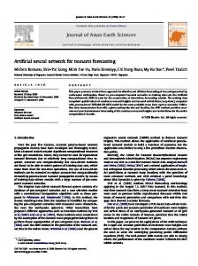
Figure 1. Structure of an artificial neural network.
methods to model time series. Artificial Neural Networks (ANNs) were introduced as efficient tools of modeling and forecasting about two decades ago. The artificial neural networks are techniques that can model, map, and demonstrate the non linear relationship of complex phenomena. The artificial neural networks are universal and highly flexible function approximators, first used in the fields of cognitive science and engineering (Kaastra and Boyd, 1996). The artificial neural networks are widely used and have become increasingly popular in a broad range of fields. The neural networks are less sensitive to the error term assumptions and can tolerate noise, chaotic components, and heavy tails better than most other methods (Masters, 1993). This paper presents a study aimed at forecasting a hydrologic time series, using neural network approaches. Stream flow forecasting using ANN The application of ANN in hydrology started in the early 1990s. A state-of-the-art review of ANN applications in hydrology can be found in the ASCE task committee report. Some applications of ANN in water resources include: precipitation–runoff modeling (Rajurkar et al., 2004; Elshorbagy and Simonovic, 2000; Tokar and Markus, 2000; Zealand et al., 1999; Fernando and Jayawardena, 1998; Hsu et al., 1995) stream flow forecasting (Moradkhani et al., 2004; Anctil et al., 2004; O¨zgu¨r, 2004), and river stage forecasting (Liong et al., 2000; Thirumalaiah and Deo, 1998; Karunanithi et al., 1994). Attempts have also been made to develop runoff hydrographs using different input parameters. Muttiah et al. (1997) used information on the drainage basin, elevation, average slope, and average annual precipitation to predict 2-year peak discharge from a watershed. Carriere et al. (1996) used ANN with a recurrent back-propagation algorithm to
The primary characteristics of ANNs are their ability to learn, distributed memory and parallel operation, eventually leading to fault tolerance. A typical three-layered network with an input layer (I), a hidden layer (H) and an output layer (O), as shown in Figure 1, is adopted in this study. Increasing the number of the hidden layers affects the complexity of the network and decreases the learning accuracy. Theoretical works have shown that a single hidden layer is sufficient for the ANNs to approximate to any complex nonlinear function (Cybenko, 1989; Hornik et al., 1989). Tang et al. (1991) recommended using one hidden layer to avoid increasing the complexity of the network. Indeed, many experimental results seem to confirm that one hidden layer may be enough for most forecasting problems (Coulibaly et al., 1999). Each layer consists of several neurons and the layers are interconnected by sets of correlation weights. The neurons receive inputs from the initial inputs or the interconnections and produce outputs by the transformation, using an adequate nonlinear transfer function. A common transfer function is the sigmoid function expressed by
. This transfer function is commonly used in back propagation networks (BPN). The training processing of neural network is essentially executed through a series of patterns. In the learning process, the interconnection weights are adjusted within input and output values. The BPN is the most representative learning model for the artificial neural network. The procedure of the BPN is that, the error at the output layer propagates backward to the input layer through the hidden layer in the network to obtain the final desired outputs. The gradient descent method is utilized to calculate the weight of the network and adjust the weight of interconnections to minimize the output error. For a network that includes n hidden layers, the error function at the output neuron can be defined as (Frederic, 2001);
(1) Where
represents the desired network output for the qth input
pattern and is the actual output of the network. Using the steepest descent gradient approach, the learning rule for a network weight in any one of the network layers is given by:
(2) Where
is the learning rate and
.
436
Int. J. Phys. Sci.
By applying Equation (2) on (1) for such a network, we can write
(3) Where
(9) Where is a small number and is the identity matrix. Substituting Equation (9) into (6) results in the LevenbergMarquardt algorithm for updating the network weights
(4) For the output layer, and
(10) Or (11)
(5) Where
g (υ )
Each term in the Jacobian matrix has the form
represent the first derivative of the transfer function
(activation function).
(12) The simplest approach to compute the derivatives in (12) is to use the approximation:
Levenberg-Marquardt back propagation algorithm Coulibaly et al. (1999) reviewed the ANN-based modeling in the hydrology over the last years and reported that about 90% of the experiments, extensively make use of the multi-layer feed-forward neural networks (FNN) trained by the back propagation (BP) algorithm. Among the modified back propagation algorithms, an early stop training approach Levenberg-Marquardt back propagation (LMBP) algorithm has widely been used for the hydrological forecasting problems, as the most powerful and accurate algorithm (Affandia et al., 2007; Aqil et al., 2007; Cobaner et al., 2008; Vongkunghae and Chumthong, 2007). The LevenbergMarquardt back propagation (LMBP) algorithm represents a simplified version of Newton’s method applied to the problem of training multilayer perceptron neural networks (MLPNNs). In Newton’s optimization algorithm, the update equation for vector
(13) Performance evaluation criteria The Correlation Coefficient (CC) and MSE are the most commonly used statistics for evaluating the performance of the ANN models (Hoła and Schabowicz, 2005; Lee, 2008; Lou and Nakai, 2001; Nasseri et al., 2008; Sedki et al., 2009; Stephen et al., 2007). Thus, to estimate the accuracy of the proposed methodology, the Mean Squared Error (MSE) and Correlation Coefficient (CC) were used as the agreement indexes:
applied on energy function E (w) is defined as (Frederick, 2001): (6)
(14)
Where, H is Hessian matrix and J is the Jacobian matrix, which is defined as follows (15)
(7) (8) And
Where
is the observed value,
is the predicted value,
the mean value of observations, and predictions.
is
is the mean value of
Model development One problem with the iterative update given in (6) is that, it requires the inversion of matrix which may be ill conditions or even singular (non-invertible). This problem can be easily resolved by the following modification
The model was developed using a back propagation ANN and its ability to forecast the monthly reservoir was tested using 21 years of monthly historical flow of Sultan Mahmud hydropower reservoir, Malaysia. The historical data for the ANN modeling is divided into
Othman and Naseri
437
Table 1. Patterns of Input Parameters used for ANN Models.
Network no. 1 2 3
Structure of model 3-X-1 3-X-1 3-X-1
No. of neurons in input layer 3 3 3
Input parameters Y(t-1) , Y(t-2) , Y(t-12) Y(t-1) , Y(t-12) , [Y(t-11)+Y(t-12)+Y(t-13)]/3 Y(t-1) , Y(t-2) , [Y(t-11)+Y(t-12)+Y(t-13)]/3
4
4-X-1
4
Y(t-1) , Y(t-2) , Y(t-12) , [Y(t-11)+Y(t-12)+Y(t13)]/3
5
4-X-1
4
Y(t-1) , Y(t-2) , Y(t-13) , [Y(t-11)+Y(t-12)+Y(t13)]/3
6
2-X-1
2
Y(t-1) , Y(t-2)
Number of neurons
Figure 2. The values of MSE vs. the number of neurons for the six networks.
two sets called the training set and the testing set. The training set is the major part of the data, that is used for training of the neural network for finding the governed pattern of data. The testing patterns are used for evaluating accuracy of the ANN trained model. Several patterns of input data have been employed to develop the optimum ANN model for the hydropower reservoir inflow. Six networks have been employed to determine the optimum ANN architecture. One hidden layer is designed for all the networks and each network was trained under several structures with different number of neurons in the hidden layer. Table 1 shows the input patterns that have been used for developing the ANN models.
RESULTS AND DISCUSSION The most important part of ANN model is its ability to forecast future events. The MSE and CC criterions are employed for evaluation of the accuracy of both training and testing procedure. The best model is chosen according to the minimum MSE and the Maximum CC.
As the aim of the ANN modeling is forecasting the reservoir inflow, the investigation of the MSE and CC among the testing results is more important. The graph of MSE with respect to the number of the neurons in the hidden layer for all the networks related to the testing process is shown in Figure 2. The behavior of the CC for the six networks associated to the testing data set can be seen in Figure 3. As can be seen from the figure, each of the network architecture has been examined with several neurons in the hidden layer. Figure 2 demonstrates that network 5 with 5 neurons is associated with the minimum MSE. The investigation of the CC graph (Figure 3) certifies that the maximum CC is related to network 5 with the 5 neurons in the hidden layer. Therefore, network 5 (that is network with model structure of 4-5-1), which includes 4 inputs, 5 neurons in hidden layer and one in output layer, was adopted as the final model. This selected ANN model was subjected to
438
Int. J. Phys. Sci.
Number of neurons Figure 3. The values of CC vs. the number of neurons for the six networks.
10
1
Validation Training
0
MSE
10
10
10
-1
-2
0
2
4
6
8
10
12
14
16
18
20
22
24
Epochs
Figure 4. MSE reduction of training and validation.
further improvement, and the early stopping approach has been employed for the training process to avoid overfitting problem. The MSE reduction of the training and
validation monitored is shown in Figure 4. The network was trained under early stopping approach and converged at MSE = 0.0188. The network forecasted
Othman and Naseri
439
Table 2. Performance of Training and Testing for the selected ANN Model.
Model 4-5-1
Training MSE 0.0188
Training CC 0.7282
Testing MSE 0.0283
Testing CC 0.7228
Figure 5. Comparison between observed and forecasted reservoir inflow using ANN model (employing training data set).
Observed (Test data)
Estimated (ANN)
Figure 6. Comparison between observed and forecasted reservoir inflow using ANN model (employing testing data set).
Using testing data set with the accuracy of MSE = 0.0283. The MSE and CC value of training and testing for selected model are presented in Table 2. Comparison between the observed and ANN estimated monthly inflow
for the training and testing data set is shown in Figures 5 and 6 respectively. It can be seen from these figures that, the agreement between the observed and estimated data are relatively good except at a few high points. In any
440
Int. J. Phys. Sci.
modeling exercise, a perfect agreement is very difficult to obtain due to the constraints and limitations in the modeling processes. Conclusion Time series forecasting has an important role for water resources planning and management. Conventionally, the researchers have employed traditional methods such as AR, ARMA, ARIMA, etc. These models provide only reasonable accuracy and suffer from the assumptions of stationary and linearity. This paper developed an ANN model for forecasting of long-term reservoir inflow. A Levenberg-Marquardt back propagation (LMBP) algorithm which includes 4 inputs, 5 neurons in hidden layer and one in output layer was developed. Result showed a relatively good agreement between the predicted and observed data. The evaluation criteria, MSE and CC values confirmed accuracy of model performance and good ability of forecasting. The model was trained and converged at MSE = 0.0188 by using training data. The ANN model can forecast the testing data set with the accuracy of MSE = 0.0283. Training and testing process show the correlation coefficient of 0.7282 and 0.7228, respectively. REFERENCES Affandia AK, Watanabe K, Tirtomihardjo H (2007). Application of an artificial neural network to estimate groundwater level fluctuation. J. Spatial Hydrol., 7: 17-32. Anctil F, Claude M, Charles P, Vazken A (2004). A soil moisture index as an auxiliary ANN input for stream flow forecasting. J. Hydrol., 286: 155-167. Aqil M, Kita I, Yano A, Nishiyama S (2007). A comparative study of artificial neural networks and neuro-fuzzy in continuous modeling of the daily and hourly behaviour of runoff. J. Hydrol., 337: 22-34. Carriere P, Mohaghegh S, Gaskari R (1996). Performance of a virtual runoff hydrograph system. J. Water Resour. Plan. Manage., 122: 421-427. Cobaner M, Information C, Haktanir T, Kisi O (2008). Prediction of Hydropower Energy Using ANN for the Feasibility of Hydropower Plant Installation to an Existing Irrigation Dam. Water Resour. Manage., 22: 757-774. Coulibaly P, Anctil F. Bobée B. (1999). Prévision hydrologique par réseaux de neurones artificiels : état de l'art. Can. J. Civ. Eng., 26(3): 293-304. Cybenko G (1989) Approximation by superpositions of a sigmoidal function. Math. Ctrl. Signals Syst. (MCSS), 2: 303–314. Elshorbagy A, Simonovic SP (2000). Performance evaluation of artificial neural networks for runoff prediction. J. Hydrol. Eng., 5: 424-427. Fernando DA, Jayawardena AW (1998). Runoff forecasting using RBF networks with OLS algorithm. J. Hydrol. Eng., 3: 203-209.
Frederic MH (2001). Principles of neurocomputing for science and engineering. McGraw Hill. New York. Hoła J, Schbowicz K (2005). Application of artificial neural networks to determine concrete compressive strength based on non-destructive tests. J. Civ. Eng., Manage., 10: 23-32. Hornik K, Stinchcombe M, White H (1989). Multilayer feed forward networks are universal approximators. Neural Netw., 2: 359-366. Hsu KL, Gupta HV, Sorooshian S (1995). Artificial neural network modeling of the rainfall–runoff process. Water Resour. Res., 31: 2517-2530. Kaastra I, Boyd M (1996). Designing a neural network for forecasting financial and economic time series. Neurocomputing, 10: 215-236. Karunanithi N, Grenney WJ, Whitley D, Bovee K (1994). Neural networks for river flow prediction. J. Comput. Civ. Eng., 8: 201–220. Lee TL (2008). Back-propagation neural network for the prediction of the short-term storm surge in Taichung harbor, Taiwan. Eng. Appl. Artif. Intell., 21: 63-72. Liong SY, Lim WH, Paudyal GN (2000). River stage forecasting in Bangladesh: Neural network approach. J. Comput. Civ. Eng., 14: 1– 8. Lou W, Nakai S (2001). Artificial Neural Network-Based Predictive Model for Bacterial Growth in a Simulated Medium of ModifiedAtmosphere-Packed Cooked Meat Products. J. Agric. Food Chem., 49: 1799-1804. Masters T (1993). Practical Neural Network Recipes in C++. Academic Press. Boston. Moradkhani H, Hoshin KL. H., Gupta V, Sorooshian S (2004). Improved streamflow forecasting using self-organizing radial basis function artificial neural networks. J. Hydrol., 295: 246–262. Muttiah RS, Srinivasan R, Allen PM (1997). Prediction of two year peak stream discharges using neural networks. J. Am. Water Resour. Assoc., 33: 625–630. Nasseri M, Asghari K, Abedini MJ (2008). Optimized scenario for rainfall forecasting using genetic algorithm coupled with artificial neural network. Expert Syst. Appl., 35: 1415-1421. O¨zgu¨r K (2004). River flow modeling using artificial neural networks. J. Hydrol. Eng., 9: 60–63. Rajurkar MP, Kothyari UC, Chaube UC (2004). Modeling of the daily rainfall–runoff relationship with artificial neural network. J. Hydrol., 285: 96–113. Sedki A, Ouazar D, Mazoudi EE (2009). Evolving neural network using real coded genetic algorithm for daily rainfall-runoff forecasting. Expert Syst. Appl., 36: 4523-4527. Smith J, Eli RN (1995). Neural-network models of rainfall–runoff process. J. Water Resour. Plan. Manage., 121: 499-508. Stephen AB, Hua-Liang W, Michael AB (2007). Generalized multiscale radial basis function networks. Neu. Netw., 20: 1081-1094. Tang Z, De Almeida C, Fishwick PA (1991). Time series forecasting using neural networks vs. Box- Jenkins methodology. Simulation, 57: 303-310. Thirumalaiah K, Deo MC (1998). River stage forecasting using artificial neural networks. J. Hydrol. Eng., 3: 26-32. Tokar AS, Markus M (2000). Precipitation–runoff modeling using artificial neural networks and conceptual models. J. Hydrol. Eng., 5: 156-161. Vongkunghae A, Chumthong A (2007). The performance comparisons of backpropagation algorithm's family on a set of logical functions. Trans. Electrical Eng., Electron. Commun., 5: 114-118. Zealand CM, Burn DH, Simonovic SP (1999). Short term stream flow forecasting using artificial neural networks. J. Hydrol., 214: 32-48.