Sep 25, 2009 - 295938, the latency of sending messages is higher than the benefit of ...... [61] Plimpton, S., Pollock, R., and Stevens, M. Particle-Mesh Ewald ...
ReSHAPE: A Framework for Dynamic Resizing of Parallel Applications
Rajesh Sudarsan
Dissertation submitted to the Faculty of the Virginia Polytechnic Institute and State University in partial fulfillment of the requirements for the degree of
Doctor of Philosophy in Computer Science and Applications
Calvin J. Ribbens, Chair Adrian Sandu Eric de Sturler Kirk Cameron Srinidhi Varadarajan
September 25, 2009 Blacksburg, Virginia
Keywords: Scheduling malleable applications, Runtime systems, Malleability in distributed-memory systems, Dynamic scheduling, High performance computing, Dynamic resizing, Application resizing framework
Copyright 2009, Rajesh Sudarsan
ReSHAPE: A Framework for Dynamic Resizing of Parallel Applications
Rajesh Sudarsan
(ABSTRACT)
As terascale supercomputers become more common, and as the high-performance computing community turns its attention to petascale machines, the challenge of providing effective resource management for high-end machines grows in both importance and difficulty. These computing resources are by definition expensive, so the cost of underutilization is also high, e.g., wasting 5% of the compute nodes on a 10,000 node cluster is a much more serious problem than on a 100 node cluster. Moreover, the high energy and cooling costs incurred in maintaining these high end machines (often millions of dollars per year) can be justified only when these machines are used to their full capacity. On large clusters, conventional jobs schedulers are hard-pressed to achieve over 90% utilization with typical job-mixes. A fundamental problem is that most conventional parallel job schedulers only support static scheduling, so that the number of processors allocated to an application cannot be changed at runtime. As a result, it is common to see jobs stuck in the queue because they require just a few more processors than are currently available, resulting in long queue wait times for applications and low overall system utilization. A more flexible and effective approach is to support dynamic resource management and scheduling, where the number of processors allocated to jobs can be expanded or contracted at runtime. This is the focus of this dissertation — dynamic resizing of parallel applications. Dynamic resizing significantly improves individual application turn-around time and helps the scheduler to achieve higher machine utilization and job throughput. This dissertation focuses on the potential benefits and challenges of dynamic resizing using ReSHAPE, a new framework for dynamic Resizing and Scheduling of Homogeneous Applications in a Parallel Environment. It also details several interesting and effective scheduling policies implemented in ReSHAPE and demonstrates their effectiveness to improve overall cluster utilization and individual application turn-around time.
Dedication
To my Mom and Dad.
iii
Acknowledgments First and foremost, I am grateful to my advisor, Dr. Calvin Ribbens, for providing me the wonderful opportunity to work with him, teaching me how to write and guiding me through the Ph.D. process. I have immensely enjoyed my work with him and also the numerous interesting conversations regarding my research. I would like to thank Dr. Kirk Cameron, Dr. Adrian Sandu, Dr. Eric de Sturler and Dr. Srinidhi Varadarajan for serving on my thesis committee and their valuable suggestions through my PhD. Furthermore, I would like to thank Dr. Kevin Shinpaugh, Laboratory of Advanced Scientific Computing and Applications and Virginia Tech Advanced Research Computing for providing financial support through Graduate Research Assistantship that enabled me to complete my degree. I would also like to thank the Tess, Rachel, Melanie, Julie, Jody, Ginger and other administrative staff at the Computer Science department for helping with all the technical and administrative related assistance. I am grateful to all my friends in the Computer Science department for their support and camaraderie. Thanks to Memo, Hari, Bharath, and Dong for their interesting conversations during our tea and coffee breaks. To my close friends in Blacksburg for just being there for me through these years. Thanks to Siva, Arun, Parthi, Vidya, Anu, Ajit, Avyukt and Pradeep. I would like to extend special thanks to Siva, Hari, Mahesh and Parthi for lending their car during my “car-less” days. I would also like to thank Wiplove, Sulabh, Pradyot, Harish, Prem, Murali, Ramkrishna and Ananth for their support. Finally, I would like to thank the most important people in my life: mom, dad, Satheesh, and Jaishree. All of these would not have been possible if not for their constant encouragement and support.
iv
Contents 1 Introduction
2
1
1.1
Motivation . . . . . . . . . . . . . . . . . . . . . . . . . . . . . . . . . . . . .
2
1.2
Problem Statement . . . . . . . . . . . . . . . . . . . . . . . . . . . . . . . .
3
1.3
Approach . . . . . . . . . . . . . . . . . . . . . . . . . . . . . . . . . . . . .
5
1.4
Organization of the document . . . . . . . . . . . . . . . . . . . . . . . . . .
6
Overview of the ReSHAPE Framework
7
2.1
Introduction . . . . . . . . . . . . . . . . . . . . . . . . . . . . . . . . . . . .
7
2.2
Related Work . . . . . . . . . . . . . . . . . . . . . . . . . . . . . . . . . . .
9
2.3
System Organization . . . . . . . . . . . . . . . . . . . . . . . . . . . . . . .
10
2.3.1
Application scheduling and monitoring module . . . . . . . . . . . . .
12
2.3.2
Resizing library and API . . . . . . . . . . . . . . . . . . . . . . . . .
15
Experimental Results . . . . . . . . . . . . . . . . . . . . . . . . . . . . . . .
18
2.4.1
Performance benefits for individual applications . . . . . . . . . . . .
21
2.4.2
Performance benefits with multiple applications . . . . . . . . . . . .
26
2.4
3 Data Redistribution
34
3.1
Introduction . . . . . . . . . . . . . . . . . . . . . . . . . . . . . . . . . . . .
34
3.2
Related Work . . . . . . . . . . . . . . . . . . . . . . . . . . . . . . . . . . .
36
3.3
Application Programming Interface (API) . . . . . . . . . . . . . . . . . . .
38
3.4
Data Redistribution . . . . . . . . . . . . . . . . . . . . . . . . . . . . . . . .
39
v
3.4.1
1D and 2D block-cyclic data redistribution for two dimensional processor grid (2D-CBR, 2D-CBC, 1D-BLKCYC). . . . . . . . . . . . .
39
One-dimensional block array redistribution across 1D and 2D processor grid (1D-BLK). . . . . . . . . . . . . . . . . . . . . . . . . . . . . . .
46
Two-dimensional block matrix redistribution for 1D and 2D processor grid (2D-BLKR and 2D-BLKC). . . . . . . . . . . . . . . . . . . . . .
50
Block-data distribution for CSR and CSC sparse matrix across 1D and 2D processor grid (2D-CSR, 2D-CSC). . . . . . . . . . . . . . . . . .
52
Experiments and Results . . . . . . . . . . . . . . . . . . . . . . . . . . . . .
56
3.4.2 3.4.3 3.4.4 3.5
4 Scheduling Resizable Parallel Applications
65
4.1
Introduction . . . . . . . . . . . . . . . . . . . . . . . . . . . . . . . . . . . .
65
4.2
Scheduling with ReSHAPE . . . . . . . . . . . . . . . . . . . . . . . . . . . .
66
4.2.1
Scheduling strategies . . . . . . . . . . . . . . . . . . . . . . . . . . .
67
4.2.2
Scheduling policies and scenarios . . . . . . . . . . . . . . . . . . . .
69
4.2.3
Scheduling policies, scenarios and strategies for priority-based applications . . . . . . . . . . . . . . . . . . . . . . . . . . . . . . . . . . .
72
Experiments and Results . . . . . . . . . . . . . . . . . . . . . . . . . . . . .
76
4.3.1
Experimental setup 1: Scheduling with NAS benchmark applications
76
4.3.2
Experimental setup 2: Scheduling with synthetic benchmark applications 82
4.3
5 Dynamic Resizing of Parallel Scientific Simulations: A Case Study Using LAMMPS
105
5.1
Introduction . . . . . . . . . . . . . . . . . . . . . . . . . . . . . . . . . . . . 105
5.2
ReSHAPE Applied to LAMMPS
5.3
Experimental Results and Discussion . . . . . . . . . . . . . . . . . . . . . . 108
. . . . . . . . . . . . . . . . . . . . . . . . 106
5.3.1
Performance Benefit for Individual MD Applications . . . . . . . . . 109
5.3.2
Performance Benefits for MD Applications in Typical Workloads . . . 111
6 Summary and Future Work
117
6.1
Summary . . . . . . . . . . . . . . . . . . . . . . . . . . . . . . . . . . . . . 117
6.2
Future Work . . . . . . . . . . . . . . . . . . . . . . . . . . . . . . . . . . . . 119 vi
List of Figures 1.1
Utilization statistics at different supercomputing sites in US . . . . . . . . .
2
2.1
Architecture of ReSHAPE. . . . . . . . . . . . . . . . . . . . . . . . . . . . .
11
2.2
State diagram for application expansion and contraction . . . . . . . . . . .
15
2.3
Original application code . . . . . . . . . . . . . . . . . . . . . . . . . . . . .
19
2.4
ReSHAPE instrumented application code . . . . . . . . . . . . . . . . . . . .
20
2.5
Running time for LU with various matrix sizes. . . . . . . . . . . . . . . . .
22
2.6
Performance with static scheduling, dynamic scheduling with file-based checkpointing, and dynamic scheduling with ReSHAPE redistribution, for five test problems. . . . . . . . . . . . . . . . . . . . . . . . . . . . . . . . . . . . . .
26
2.7
Processor allocation history for workload W1. . . . . . . . . . . . . . . . . .
28
2.8
Total processors used for workload W1. . . . . . . . . . . . . . . . . . . . . .
28
2.9
Processor allocation history for workload W2. . . . . . . . . . . . . . . . . .
30
2.10 Total processors used for workload W2. . . . . . . . . . . . . . . . . . . . . .
31
2.11 Processor allocation history for workload W3 with ReSHAPE . . . . . . . .
33
2.12 Processor allocation history for workload W3 with static scheduling . . . . .
33
3.1
P = 4 (2 × 2) and Q = 12 (3 × 4). Data layout in source and destination processors. . . . . . . . . . . . . . . . . . . . . . . . . . . . . . . . . . . . . .
41
Creating of communication schedule (CSend) from Initial Data Processor Configuration table (IDPC), Final Data Processor Configuration table (FDPC) and CRecv table. . . . . . . . . . . . . . . . . . . . . . . . . . . . . . . . . . .
42
3.3
Redistribution time (P = 16, Q=32, blocksize = 512x512) . . . . . . . . . .
58
3.4
Redistribution overhead (P = 8, Q=64, blocksize = 512x512) . . . . . . . . .
59
3.2
vii
3.5
Redistribution time (P = 32, Q=16, blocksize = 512x512) . . . . . . . . . .
59
3.6
Redistribution time (P = 64, Q=32, blocksize = 512x512) . . . . . . . . . .
60
3.7
Redistribution time (P = 4, Q=64, blocksize = 512x512) . . . . . . . . . . .
61
3.8
Redistribution time (P = 8, Q=32, blocksize = 512x512) . . . . . . . . . . .
61
3.9
Redistribution time (P = 16, Q=32, blocksize = 512x512) . . . . . . . . . .
62
4.1
Comparing job completion time for individual applications executed with FCFS-LI-Q scheduling scenario and static scheduling policy. . . . . . . . . .
78
Comparing performance of FCFS-LI-Q scheduling scenario and static scheduling with backfill policy. . . . . . . . . . . . . . . . . . . . . . . . . . . . . . .
79
Average wait time and average execution time for all the applications in the job mix. . . . . . . . . . . . . . . . . . . . . . . . . . . . . . . . . . . . . . .
80
Average completion time and overall system utilization for all applications in job mix. . . . . . . . . . . . . . . . . . . . . . . . . . . . . . . . . . . . . . .
81
Job completion time for FT and IS applications with different scheduling scenarios . . . . . . . . . . . . . . . . . . . . . . . . . . . . . . . . . . . . . .
83
Job completion time for CG and LU applications with different scheduling scenarios . . . . . . . . . . . . . . . . . . . . . . . . . . . . . . . . . . . . . .
84
4.7
Speedup curve. . . . . . . . . . . . . . . . . . . . . . . . . . . . . . . . . . .
86
4.8
Average completion time for various scheduling scenarios. . . . . . . . . . . .
87
4.9
Average execution time for various scheduling scenarios.
. . . . . . . . . . .
88
4.10 Average execution time by job size for various scheduling scenarios. . . . . .
88
4.11 Average queue time for various scheduling scenarios. . . . . . . . . . . . . . .
89
4.12 Average queue wait time by job size for various scheduling scenarios. . . . .
90
4.13 Average system utilization for various scheduling scenarios. . . . . . . . . . .
90
4.14 Average completion time for a workload where all large jobs arrive together at the beginning of the trace. . . . . . . . . . . . . . . . . . . . . . . . . . .
91
4.15 Average completion time for a workload where all large jobs arrive together at the end of the trace. . . . . . . . . . . . . . . . . . . . . . . . . . . . . . .
92
4.16 Average completion time for workloads with varying percentage of resizable jobs. . . . . . . . . . . . . . . . . . . . . . . . . . . . . . . . . . . . . . . . .
94
4.17 Average completion time for small, medium and large jobs. . . . . . . . . . .
94
4.2 4.3 4.4 4.5 4.6
viii
4.18 Average execution time for workloads with varying percentages of resizable jobs. . . . . . . . . . . . . . . . . . . . . . . . . . . . . . . . . . . . . . . . .
95
4.19 Average queue time for workloads with varying percentages of resizable jobs.
96
4.20 Average queue time by job size for workloads with varying percentages of resizable jobs . . . . . . . . . . . . . . . . . . . . . . . . . . . . . . . . . . .
97
4.21 Average execution time by job size for workloads with varying percentages of resizable jobs. . . . . . . . . . . . . . . . . . . . . . . . . . . . . . . . . . . .
97
4.22 Average system utilization for workload with varying percentages of resizable jobs. . . . . . . . . . . . . . . . . . . . . . . . . . . . . . . . . . . . . . . . .
98
4.23 Average completion time.
. . . . . . . . . . . . . . . . . . . . . . . . . . . .
99
4.24 Average completion time by priority. . . . . . . . . . . . . . . . . . . . . . .
99
4.25 Average completion time grouped by size for gold jobs. . . . . . . . . . . . . 100 4.26 Average execution time . . . . . . . . . . . . . . . . . . . . . . . . . . . . . . 100 4.27 Average execution time for large, medium and small sized jobs . . . . . . . . 101 4.28 Average queue wait time . . . . . . . . . . . . . . . . . . . . . . . . . . . . . 101 4.29 Average queue wait time for gold and platinum users . . . . . . . . . . . . . 102 4.30 Average queue wait time for large, medium and small sized jobs for platinum users . . . . . . . . . . . . . . . . . . . . . . . . . . . . . . . . . . . . . . . . 102 4.31 Average system utilization . . . . . . . . . . . . . . . . . . . . . . . . . . . . 103 5.1
LAMMPS input script (left) and restart script (right) extended for ReSHAPE .108
5.2
Identifying the execution sweet spot for LAMMPS. . . . . . . . . . . . . . . 110
5.3
Processor allocation and overall system utilization for a job mix of a single resizable LAMMPS job with static jobs. . . . . . . . . . . . . . . . . . . . . 113
5.4
Processor allocation and overall system utilization for a job mix of resizable NAS benchmark jobs with a single resizable LAMMPS job. . . . . . . . . . . 114
5.5
Processor allocation and overall system utilization for a job mix of multiple resizable NAS benchmark and LAMMPS jobs. . . . . . . . . . . . . . . . . . 115
ix
List of Tables 2.1
Applications used to illustrate the potential of ReSHAPE for individual applications. . . . . . . . . . . . . . . . . . . . . . . . . . . . . . . . . . . . . .
21
2.2
Redistribution overhead for expansion and contraction for different matrix sizes. 22
2.3
Iteration and redistribution for LU on problem size 16000. . . . . . . . . . .
25
2.4
Processor configurations for each of 10 iterations with ReSHAPE. . . . . . .
25
2.5
Workloads for job mix experiment using NAS parallel benchmark applications. 27
2.6
Job turn-around time . . . . . . . . . . . . . . . . . . . . . . . . . . . . . . .
29
2.7
Job turn-around time . . . . . . . . . . . . . . . . . . . . . . . . . . . . . . .
32
3.1
Redistribution overhead for expansion and contraction for 16K x 16K matrix with block size 512x512. . . . . . . . . . . . . . . . . . . . . . . . . . . . . .
57
3.2
Redistribution overhead for expansion and contraction for sparse matrices. .
63
3.3
Redistribution overhead for processor contraction. P=16, Q=8 . . . . . . . .
64
4.1
Job trace using NAS parallel benchmark applications.
77
4.2
Summary of job completion time and job execution time for various scenarios. 92
4.3
Queue wait time for various scenarios.
. . . . . . . . . . . . . . . . . . . . .
93
4.4
Summary of job completion time for individual runs. . . . . . . . . . . . . .
93
4.5
Average completion time for jobs with and without priority (50% resizable jobs, 50% high priority jobs) . . . . . . . . . . . . . . . . . . . . . . . . . . . 104
5.1
Job workloads and descriptions . . . . . . . . . . . . . . . . . . . . . . . . . 109
5.2
The table shows the number of atoms for different LAMMPS problem sizes. . 110
5.3
Performance improvement in LAMMPS due to resizing. Time in secs. . . . . 110 x
. . . . . . . . . . . .
5.4
Performance results of LAMMPS jobs for jobmix experiment. Time in secs. . 112
xi
Chapter 1 Introduction Applications in science and engineering require enormous computational resources to solve large problems within a reasonable time frame. Supercomputers, with thousands of processors and terabytes of memory, provide the resources to execute such computational science and engineering (CSE) applications. Lately, computational grids and commodity clusters have provided a low cost alternative to custom built supercomputers for large scale CSE. Grids are loosely-coupled heterogeneous internet systems that act as a single computing facility. Each computing unit (or node) in a grid has its own resource manager and can be located at different sites within various administrative domains. Clusters are tightly-coupled homogeneous computing systems built using a number of off-the-shelf commodity computers. The nodes in these systems are connected together via a high speed interconnect and act as a single unified resource. Multiprocessors can be architecturally classified into two main categories — shared memory multiprocessors (SMP) and distributed memory clusters. All the processors in a shared memory multiprocessor access a single unified memory whereas in a distributed memory cluster, the processors have their own memory and communicate using messages. A centralized resource manager administers processor allocation in a cluster. Clusters are becoming the foremost choice for building supercomputers and they account for 82% of the top 500 fastest supercomputers in the world [77]. According to the most recent list of Top 500 supercomputers, released in June 2009, 470 out of these 500 supercomputers have at least 2000 processors. Even though clusters provide a viable low cost alternative to customized supercomputers, it still costs millions of dollars to build them plus hundreds of thousands of dollars every year for maintanence,power and cooling costs. Thus it becomes imperative to use these machines to their maximum potential to do useful scientific research. The challenge of providing effective resource management for these high-end machines grows both in importance and difficulty as the number of processors in a cluster increases. Techniques such as backfilling [41, 54, 67], gang scheduling [20, 24, 85, 89], co-scheduling [90] and processor virtualization [39, 35] try to provide effective resource management and improve the overall system utilization. But even with these techniques it is difficult to get more than 1
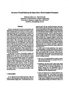
2 90% utilization. Figure 1.1 shows recent utilization statistics [16] over a period of one year for some of the high-end machines at different supercomputing sites across US. The average utilization at these sites is around 70%. Most of these sites also have an associated cost model, which quantifies the value of a cpu hour taking into account both initial and ongoing expenses. . Even if they charge a meager sum of 30 cents per cpu hour, a 30% wastage of cpu resources can amount to almost one million dollars every year.
Figure 1.1: Utilization statistics at different supercomputing sites in US
1.1
Motivation
As terascale supercomputers become common, and as the high-performance computing (HPC) community turns its attention towards petascale machines, there is an increasing interest in developing effective resource management for these large scale machines. High capability computing resources are by definition expensive, so the cost of underutilization is high. Furthermore, high capability computing is characterized by long-running, high node-count jobs. A job-mix dominated by a relatively small number of such jobs is notoriously difficult to schedule effectively on a large-scale cluster. A fundamental problem is that conventional parallel schedulers are static, i.e., once a job is allocated a set of processors, it continues to use those processors until it finishes execution. Under static scheduling, jobs will not be scheduled for execution until the number of processors requested by an application are available in the system. Thus, it is common for jobs to be stuck in the queue because they require just a few more processors than are currently available. With a priority-based static scheduling policy, high priority jobs are scheduled quickly but only at the expense of blocking
3 on suspending low priority jobs. Also, due to the unpredictability in job arrival times and varying resource requirements, static scheduling can result in idle system resources thereby reducing the overall system throughput. Dynamic scheduling [65] mitigates the above described limitations of static scheduling, enabling schedulers to reallocate resources to parallel applications at runtime. To manage cluster resources efficiently, we need schedulers that support dynamic scheduling in order to achieve the goals such as the following: • Improve the overall cluster utilization and system throughput • Be able to reconfigure low priority jobs in order to schedule high priority jobs or to meet an advance reservation commitment. • Improve an application’s turn-around time by starting its execution on a smaller processor set and later acquiring more processors depending upon the application’s performance. As a result, the jobs won’t be stuck in the queue waiting for a larger number of processors to become available. • Provide application-aware resource management. For example, if an application can add processors only in steps of fixed pre-determined values (e.g., size of processor row or processor column in a 2D topology or in powers of 2), then the scheduler should meet those application constraints when allocating processors. • Be able to probe and identify the execution sweet spot for a particular application and problem. A sweet spot could be defined as a processor count where an increase in the number of processors will not further improve performance. The focus of our research is on dynamically reconfiguring parallel applications to use a different number of processes, i.e., on dynamic resizing of parallel applications.
1.2
Problem Statement
From the above discussion, we define the problem statement for this research as follows: How to design and implement an efficient software infrastructure to support dynamic resizing for parallel applications and how to use this framework to resize parallel applications so that the overall system throughput and an individual application’s turn-around time is improved?
4 We identify four main tasks involved in the dynamic processor reconfiguration of an application: application scheduling, resource management, processor remapping and data redistribution. As a guideline for our research and to answer the above problem statement, we have formulated the following research questions: Question 1: What new scheduling and resource management policies are possible with dynamic resizing? A conventional scheduler supports different policies like backfill, priority-based scheduling, and dynamic partition policy. More scheduling policies become available by combining resizing with existing scheduler policies. A study to compare the effectiveness of these policies with static scheduling is required. We need to measure the system throughput and application turn-around time with dynamic resizing. Question 2: How can an application’s global state be efficiently redistributed? When an application’s processor allocation is dynamically reconfigured, all the global data associated with the application must be redistributed to the new processor set. An efficient algorithm to reduce the data redistribution overhead is necessary. We need to identify the various data structures used in real scientific applications and devise an efficient technique to redistribute them. Question 3: What are the different classes of applications that will benefit from dynamic resizing? Dynamic processor reconfigurability is applicable to only those applications that can execute on different partition sizes. Thus, it is necessary to identify the different classes of applications that can be executed using schedulers that support dynamic reconfiguration. Question 4: What type of software framework is required to allow application developers to exploit the benefits of dynamic resizing? How much application code modification is required? Is it possible to integrate this framework with existing cluster schedulers? Existing parallel applications must be modified to support dynamic reconfiguration. A well defined software framework will reduce the burden on an application programmer to perform extensive code modification to support dynamic reconfiguration. Also, this framework must be integrated with existing cluster schedulers to make it commercially viable. We need to identify the challenges involved with such an integration.
5 Question 5: How can the scheduler measure and predict an application’s performance? How should an application be reconfigured based on its performance? An application’s performance determines how it should be reconfigured. We need to devise a method to predict and track the performance results of an application so that the scheduler can make better reconfiguration decisions.
1.3
Approach
We use dynamic application scheduling to effectively manage the available cluster resources (among the queued and executing applications) in a way that is transparent to users. Using dynamic scheduling, schedulers can add or remove processors from an application at runtime, i.e., dynamically resize an application. With dynamic resizing, schedulers can start execution of a queued job on a smaller partition of processors and add more processors later, thereby resulting in higher machine utilization and job throughput. Alternatively, the scheduler could add unused processors to a particular job in order to help that job finish earlier, thereby freeing up resources for waiting jobs. Schedulers could also expand or contract the processor allocation for an already running application in order to accommodate higher priority jobs, or to meet a quality of service (QoS) or advance reservation commitment. Dynamic resizing improves the job turn-around time by allowing the scheduler to start execution of an application at an earlier time as compared to static scheduling. In order to explore the potential benefits and challenges of dynamic resizing, we propose ReSHAPE, a framework for dynamic Resizing and Scheduling of Homogeneous Applications in a Parallel Environment. The ReSHAPE framework includes the following: 1. A parallel scheduling and resource management system. 2. Data redistribution algorithms and a runtime library. 3. A programming model and API. The resizing library in ReSHAPE includes efficient one-and two-dimensional data redistribution algorithm [69] for dense and sparse matrices. The 1D and 2D block-cyclic data redistribution algorithms for two dimensional processor grids is an extension to the 1D data redistribution algorithms originally proposed by Park et al. [57]. The programming model in ReSHAPE is simple enough to port an existing code to the new system without requiring unreasonable re-coding. Runtime mechanisms include support for releasing and acquiring processors and efficiently redistributing an application state to a new set of processors. The scheduling mechanism in ReSHAPE exploits resizability to increase system throughput and
6 reduce job turn around time. The framework includes different scheduling policies and scenarios [71] to support both regular and priority-based scheduling. These characteristics make ReSHAPE usable and effective. In this research we consider parallel applications that are malleable [22] or resizable, i.e., the number of processors allocated to a parallel application can change at runtime.
1.4
Organization of the document
The rest of this dissertation is organized as follows. Chapter 2 presents a design overview of ReSHAPE with some early performance results used to illustrate the potential of dynamic resizing. It describes in detail the different components in ReSHAPE and gives an overview of the programming model supported by ReSHAPE [70]. Chapter 3 discusses the various data redistribution algorithms implemented in ReSHAPE and shows performance results compared to some existing data redistribution algorithms [69]. Chapter 4 describes in detail the different scheduling policies, scenarios and strategies implemented in ReSHAPE [71]. The chapter also discusses the performance prediction model used in ReSHAPE to make resizing decisions. Chapter 5 demonstrates the effectiveness of ReSHAPE using a widely used scientific production molecular dynamics code, LAMMPS [72]. Finally, Chapter 6 summarizes the entire research and discusses directions for future research. Related works for this dissertation are presented as separate sections within individual chapters.
Chapter 2 Overview of the ReSHAPE Framework 2.1
Introduction
Processor counts on parallel supercomputers continue to rise steadily. Thousands of processor cores are becoming almost common place in high-end machines. Although the increased use of multicore nodes means that node-counts may rise more slowly, it is still the case that cluster schedulers and cluster applications have more and more processor cores to manage and exploit. As the sheer computational capacity of these high-end machines grows, the challenge of providing effective resource management grows as well—in both importance and difficulty. High capability computing platforms are by definition expensive, so the cost of underutilization is high. Failing to use 5% of the processor cores on a 100,000 core cluster is a much more serious problem than on a 100 core cluster. Furthermore, high capability computing is characterized by long-running, high processor-count jobs. A job-mix dominated by a relatively small number of such jobs is more difficult to schedule effectively on a large cluster. In almost four years of experience operating System X, a terascale system at Virginia Tech, we have observed that conventional schedulers struggle to achieve over 90% utilization with typical job-mixes, consisting of a high percentage of jobs requiring a large number of processors. A fundamental problem is that conventional parallel schedulers are static; once a job is allocated a set of resources, it continues to use those same resources until it finishes execution. A more flexible and effective approach would support dynamic resource management and scheduling, where the set of processors allocated to jobs can be expanded or contracted at runtime. This is the focus of our research—dynamically reconfiguring (resizing) parallel applications. There are many ways in which dynamic resizing can improve the utilization of clusters as well as reduce the time-to-completion (queue waiting time plus execution time) of individual
7
8 cluster jobs. From the perspective of the scheduler, dynamic resizing can yield higher machine utilization and job throughput. For example, with static scheduling it is common to see jobs stuck in the queue because they require just a few more processors than are currently available. With resizing, the scheduler may be able to launch a job earlier (i.e., back-fill ), by squeezing the job onto the processors that are available, and then possibly adding more processors later. Alternatively, the scheduler can add unused processors to a job so that the job finishes earlier, thereby freeing up resources earlier for waiting jobs. Schedulers can also expand or contract the processor allocation for an already running application in order to accommodate higher priority jobs, or to meet a quality of service or advance reservation deadline. More ambitious scenarios are possible as well, where, for example, the scheduler gathers data about the performance of running applications in order to inform decisions about who should get extra processors or from whom processors should be harvested. Dynamic resizing also has potential benefits from the perspective of an individual job. A scheduling mechanism that allows a job to start earlier or gain processors later can reduce the time-to-completion for that job. Applications that consist of multiple phases, some of which are more computationally intensive or scalable than others, can benefit from resizing to the most appropriate processor count for each phase. Another possible way to exploit resizability is in identifying a processor count sweet spot for a particular job. For any (fixed problem-size) parallel application, there is a point beyond which adding more processors does not help. Dynamic resizing gives applications and schedulers the opportunity to probe for processor-count sweet spots for a particular application and problem size. In order to explore the potential benefits and challenges of dynamic resizing, we have developed ReSHAPE, a framework for dynamic Resizing and Scheduling of Homogeneous Applications in a Parallel Environment. The ReSHAPE framework includes a programming model and API, a runtime library containing methods for data redistribution, and a parallel scheduling and resource management system. In order for ReSHAPE to be a usable and effective framework, there are several important criteria which these components should meet. The programming model needs to be simple enough so that existing code can be ported to the new system without an unreasonable re-coding burden. Runtime mechanisms must include support for releasing and acquiring processors and for efficiently redistributing application state to a new set of processors. The scheduler must exploit resizability to increase system throughput and reduce job turn around time. In [70] we described the initial design of ReSHAPE and illustrated its potential with some simple experiments. In this chapter we describe the evolved design more fully, along with the application programming interface (API) and example ReSHAPE-enabled code, and give new and more complete experimental results which demonstrate the performance improvements possible with our framework. We focus here on improving the performance of iterative applications. However, the applicability of ReSHAPE can be extended to non-iterative applications as well. The main contributions of our framework include: 1. a scheduler which dynamically manages resources for parallel applications executing in
9 a homogeneous cluster; 2. an efficient runtime library for processor remapping and data redistribution; 3. a simple programming model and easy-to-use API for modifying existing scientific applications to exploit resizability. The rest of the chapter is organized as follows. Section 2.2 presents related work in the area of dynamic processor allocation. Section 2.3 describes the design and implementation details of the ReSHAPE framework, including the API. Section 2.4 presents the results of several experiments, which illustrate and evaluate the performance gains possible with our framework.
2.2
Related Work
Dynamic scheduling of parallel applications has been an active area of research for several years. Much of the early work targets shared memory architectures although several recent efforts focus on grid environments. Feldmann et al. [23] propose an algorithm for dynamic scheduling on parallel machines under a PRAM programming model. McCann et al. [46] propose a dynamic processor allocation policy for shared memory multiprocessors and study space-sharing vs. time-sharing in this context. Julita et al. [11] present a scheduling policy for shared memory systems that allocates processors based on the performance of the application. Moreira and Naik [48] propose a technique for dynamic resource management on distributed systems using a checkpointing framework called Distributed Resource Management Systems (DRMS). The framework supports jobs that can change their active number of tasks during program execution, map the new set of tasks to execution units, and redistribute data among the new set of tasks. DRMS does not make reconfiguration decisions based on application performance however, and it uses file-based checkpointing for data redistribution. A more recent work by Kal`e [35] achieves reconfiguration of MPI-based message passing programs. However, the reconfiguration is achieved using Adaptive MPI (AMPI), which in turn relies on Charm++ [39] for the processor virtualization layer, and requires that the application be run with many more threads than processors. Weissman et al. [87] describe an application-aware job scheduler that dynamically controls resource allocation among concurrently executing jobs. The scheduler implements policies for adding or removing resources from jobs based on performance predictions from the Prophet system [86]. All processors send data to the root node for data redistribution. The authors present simulated results based on supercomputer workload traces. Cirne and Berman [10, 9] use the term moldable to describe jobs that can adapt to different processor sizes. In their work the application scheduler AppLeS selects the job with the least estimated turn-around time out of a set of moldable jobs, based on the current state of the parallel computer. They also propose a model for scheduling moldable jobs on
10 supercomputers [9]. Possible processor configurations are specified by the user, and the number of processors assigned to a job does not change after job-initiation time. Vadhiyar and Dongarra [81, 82] describe a user-level checkpointing framework called Stop Restart Software (SRS) for developing malleable and migratable applications for distributed and Grid computing systems. The framework implements a rescheduler which monitors application progress and can migrate the application to a better resource. Data redistribution is done via user-level file-based checkpointing. El Maghraoui et al. [37] describe a framework to enhance the performance of MPI applications through process checkpointing, migration and load balancing. The infrastructure uses a distributed middleware framework that supports resource-level and application-level profiling for load balancing. The framework continuously evaluates application performance, discovers new resources, and migrates all or part of an application to better resources. Huedo et al. [33] also describe a framework, called Gridway, for adaptive execution of applications in Grids. Both of these frameworks target Grid environments and aim at improving the resources assigned to an application by replacement rather than increasing or decreasing the number of resources. The ReSHAPE framework described in this chapter has several aspects that differentiate it from the above work. ReSHAPE is designed for applications running on distributedmemory clusters. Like [10, 87], applications must be malleable in order to take advantage of ReSHAPE but in our case the user is not required to specify the legal partition sizes ahead of time. Instead, ReSHAPE can dynamically calculate partition sizes based on the run-time performance of the application. ReSHAPE has an additional advantage of being able to change dynamically an application’s partition size whereas the framework described by Cirne and Berman [10] needs to decide on the partition size before starting an application’s execution. Our framework uses neither file-based checkpointing nor a single node for redistribution. Instead, we use an efficient data redistribution algorithm which remaps data on-the-fly using message-passing over the high-performance cluster interconnect. Finally, we evaluate our system using experimental data from a real cluster, allowing us to investigate potential benefits both for individual job turn-around time and overall system utilization and throughput.
2.3
System Organization
The architecture of the ReSHAPE framework, shown in Figure 2.1, consists of two main components. The first component is the application scheduling and monitoring module which schedules and monitors jobs and gathers performance data in order to make resizing decisions based on application performance, available system resources, resources allocated to other jobs in the system, and jobs waiting in the queue. The basic design of the application scheduler was originally part of the DQ/GEMS project [74]. The initial extension of DQ to support resizing was done by Chinnusamy and Swaminathan [6, 73]. The second component of the framework consists of a programming model for resizing applications. This includes
11 a resizing library and an API for applications to communicate with the scheduler to send performance data and actuate resizing decisions. The resizing library includes algorithms for mapping processor topologies and redistributing data from one processor topology to another. The library is implemented using standard MPI-2 [49] functions and can be used with any MPI-2 implementation. The resizing library currently includes redistribution algorithms for generic one-dimensional block data distribution, one- and two-dimensional block-cyclic data distribution and block data distribution for sparse matrices in CSR format (see Section 2.3.2), but it can be extended to support other data structures and other redistribution algorithms.
Figure 2.1: Architecture of ReSHAPE. ReSHAPE targets applications that are homogeneous in two important ways. First, our approach is best suited to applications where data and computations are relatively uniformly
12 distributed across processors. Second, we assume that the application is iterative, with the amount of computation done in each iteration being roughly the same. While these assumptions do not hold for all large-scale applications, they do hold for a significant number of large-scale scientific simulations. Hence, in the experiments described in this dissertation, we use applications with a single outer iteration, and with one or more large computations dominating each iteration. Our API gives programmers a simple way to indicate resize points in the application, typically at the end of each iteration of the outer loop. At resize points, the application contacts the scheduler and provides performance data to the scheduler. The metric used to measure performance is the time taken to compute each iteration.
2.3.1
Application scheduling and monitoring module
The application scheduling and monitoring module includes five components, each executed by a separate thread. The different components are System Monitor, Application Scheduler, Job Startup, Remap Scheduler, and Performance Profiler. We describe each component in turn, along with a simple example of scheduling scenarios that are implemented in our current system. It is important to note that the ReSHAPE framework can easily be extended to support more sophisticated scheduling policies and scenarios. Chapter 4 describes several more sophisticated scenarios in detail. System Monitor. An application monitor is instantiated on every compute node to monitor the status of an application executing on the node and report the status back to the System Monitor. If an application fails due to an internal error (i.e., the monitor receives an error signal) or finishes its execution successfully, the application monitor sends a job error signal or a job end signal to the System Monitor. The System Monitor then deletes the job and recovers the application’s resources. For each application, only the monitor running on the first node of its processor set communicates with the System Monitor. Application Scheduler. An application is submitted to the scheduler for execution using a command line submission process. The scheduler enqueues the job and waits for the requested number of processors to become available. As soon as the resources become available, the scheduler selects the compute nodes, marks them as unavailable in the resource pool, and sends a signal to the job startup thread to begin execution. The initial implementation of ReSHAPE supported two basic resource allocation policies, First Come First Served (FCFS) and simple backfill. A job is backfilled if sufficient processors are available and the wallclock time of the job (supplied by the user) is smaller than the expected start time of the first job in the queue. Job Startup. Once the Application Scheduler allocates the requested number of processors to a job, the job startup thread initiates an application startup process on the set of processors assigned to the job. The startup thread sends job start information to the application monitor executing on the first node of the allocated set. The application monitor sends job error or job completion messages back to the System Monitor.
13 Performance Profiler. At every resize point, the Remap Scheduler receives performance data from a resizable application. The performance data includes the number of processors used, time taken to complete the previous iteration, and the redistribution time for mapping the distributed data from one processor set to another, if any. The Performance Profiler maintains lists of the various processor sizes each application has run on and the performance of the application at each of those sizes. The Profiler also maintains a list of possible shrink points of various applications and the anticipated impact on the application’s performance. Each entry in the shrink points list consists of job id of an application, number of processors each application can relinquish and the expected performance degradation which would result from this change. Note that applications can only contract to processor configurations on which they have previously run. Remap Scheduler. The point between two subsequent iterations in an application is called a resize point. After each iteration, a resizable application contacts the Remap Scheduler with its latest iteration time. The Remap Scheduler contacts the Performance Profiler to retrieve information about the application’s past performance and decides to expand or shrink the number of processors assigned to an application according to the scheduling policies enforced by the particular scheduler. As an example of a simple but effective scheduling policy, our initial implementation of ReSHAPE increased the number of processors given to an application if 1. there are idle processors in the system, and 2. there are no jobs waiting to be scheduled on the idle processors, and 3. either the job has not yet been expanded, or the system predicts—based on performance results held by the Performance Profiler—that additional processors will help performance. The size and topology of the expanded processor set can be problem and application dependent. Furthermore, at job submission time applications can indicate through the API if they prefer a particular processor topology, e.g., a rectangular processor grid, power-of-2 or arbitrary. In case an application prefers “nearly-square” topologies, additional processors are added to the smallest row or column of the existing topology. For power-of-2 processor topology, number of processors are doubled and in the case of arbitrary topology, a fixed number of additional processors are allocated for expansion. The processor expansion size for arbitrary topology is set as a configuration parameter in the Remap Scheduler. Continuing with the simple scheduling scenario, the Remap Scheduler decides to contract the number of processors for an application if it has previously run on a smaller processor set and 1. at the last resize point, the application expanded its processor set to a size that did not provide any performance benefit, or
14 2. there are applications in the queue waiting to be scheduled. In this example, the scheduler implements a policy that favors both queued and running applications. By favoring queued applications, the scheduler attempts to minimize the queue wait time. When an application contacts the scheduler at its resize point, the Remap Scheduler checks whether it can schedule the first queued job by contracting one or more running applications. If it can, then the scheduler contracts applications in ascending order of performance impact: applications expected to suffer the least impact from contraction, based on previous performance data, lose processors first. The Remap Scheduler checks whether the current job is one of the candidates that needs to be contracted. If it is, then the application is contracted either to its starting processor size or to one of its previous processor allocations depending upon the number of processors required to schedule the queued job. If more processors are required, then the scheduler will harvest additional processors when other applications check in at their resize point. If the scheduler chooses not to contract the current application, then it predicts whether the application will benefit from additional processors. If so, and if there are processors available with no queued applications, then the scheduler expands the application to its next possible processor set size. If the application’s performance was hurt by the last expansion, then it is contracted to its previous smaller processor allocation. If none of the above condition are met, then the scheduler leaves the application’s processor allocation unchanged. A simple performance model is used to predict an application’s performance using past results. Based on the prediction, the scheduler decides whether an application should expand, contract or maintain its current processor size. The model uses performance results from an application’s last three resize intervals to construct a quadratic interpolant of the performance of the application over that range of processor allocations. A resize interval is the change in the number of processors between two resize points. Currently we use the application’s iteration time as a measure of performance. We use the slope of the interpolant at the current processor set size as a predictor of potential performance improvement. If the slope exceeds a pre-determined threshold (currently 0.2), then the model predicts that adding more processors will benefit the application’s performance. Otherwise, it predicts that the application will have little or no benefit from adding additional processors. In the case of applications that have only two resize intervals, the model predicts performance using a straight line. The prediction model is not used when the application has only one or no resize intervals. We emphasize again that a more sophisticated prediction model and policies are possible. Indeed, a significant motivation for ReSHAPE in general, and the Performance Profiler in particular, is to serve as a platform for research into more sophisticated resizing strategies. Chapter 4 describes and evaluates a few of the scheduling strategies made possible by ReSHAPE.
15
Figure 2.2: State diagram for application expansion and contraction
2.3.2
Resizing library and API
The ReSHAPE resizing library includes routines for changing the size of the processor set assigned to an application and for mapping processors and data from one processor set to another. An application needs to be re-compiled with the resize library to enable the scheduler to add or remove processors dynamically to or from the application. During resizing, rather than suspending the job, the application execution control is transferred to the resize library which maps the new set of processors to the application and redistributes the data (if any). Once mapping is completed, the resize library returns control back to the application and the application continues with its next iteration. The application programmer needs to indicate the globally distributed data structures and variables so that they can be redistributed to the new processor set after resizing. Figure 2.2 shows the different stages of execution required for changing the size of the processor set for an application.
16 Processor remapping At resize points, if an application is allowed to expand to more processors, the response from the Remap Scheduler includes the size and the list of processors to which an application should expand. The resizing library spawns new processes on these processors using the MPI-2 function MPI Comm spawn multiple called from within the library. The spawned child processes and the parent processes are merged together and a new communicator is created for the expanded processor set. The old MPI communicator is replaced with the newly created expanded intra-communicator. A call to the redistribution routine remaps the globally distributed data to the new processor set. If the scheduler tells an application to contract, then the application first redistributes its global data to the smaller processor subset, replaces the current communicator with the previously stored MPI communicator for the application and terminates any additional processes present in the old communicator. The resizing library notifies the Remap Scheduler about the number of nodes relinquished by the application. The current implementation of the remap scheduler supports processor configurations for three types of processor topologies: arbitrary, two-dimensional (nearlysquare topology), and powers-of-2 processor topology. Data redistribution Chapter 3 discusses the data redistribution in detail. Here we give only a brief overview. The data redistribution library in ReSHAPE uses an efficient algorithm for redistributing block and block-cyclic arrays between processor sets organized in a 1-D (row or column format) or 2-D processor topology. The algorithm used for redistributing 1D and 2D block-cyclic data uses a table-based technique to develop an efficient and contention-free communication schedule for redistributing data from P to Q processors, where P 6= Q. The initial (existing) data layout and the final data layout are represented in a tabular format. The number of rows in the initial and final data layout tables is equal to the least common multiple of the number of processor rows in the old and resized processor set. A least common multiple of the number of processor columns in the old and resized processor set determines the number of columns in the initial and final data layout tables. A third table—called the communication send table—represents the mapping between the initial and the final data layout, where columns correspond to the processors in the source processor set. Each row in this table represents a single communication step in which data blocks from the initial layout are transferred to their destination processors indicated by the individual entries in the communication send table. Another table—called the communication receive table—is derived from the communication send table, and stores the mapping information similar to the communication send table. In this table, the columns correspond to the destination processor set and each entry in the table indicates the source processor of the data stored in that location. The communication send and receive tables are rearranged such that the maximum possible number of processors are either sending or receiving at each communication step (depends whether P > Q or P < Q)
17 without any node contention. Our current implementation of the checkerboard redistribution algorithm for 2D processor topology requires that the number of processors evenly divides the problem size. Sudarsan and Ribbens [69] describe the redistribution algorithm for a 2-D processor topology in detail. The one-dimensional block redistribution algorithm uses a linked list to represent the communication send and receive schedule. Each processor maintains an individual list for the communication send and receive schedule that stores the processor rank and the amount of data that needs to be sent or received from that processor. Similar to the block-cyclic redistribution algorithm, the block redistribution algorithm ensures that the maximum possible number of processors are either sending or receiving at each communication step. Application Programming Interface (API) A simple API allows user codes to access the ReSHAPE framework and library. These functions provide access to the main functionality of the resizing library by contacting the scheduler, remapping the processors after an expansion or a contraction, and redistributing the data. The API provides interfaces to support both C and Fortran language bindings. The API defines a global communicator called RESHAPE COMM WORLD required to communicate among the MPI processes executing within the ReSHAPE framework. This communicator is automatically updated after each resizing decision and reflects the most recent group of active MPI processes for an application. The core functionality of the framework is accessed through the following interfaces. • reshape Init (struct ProcessorTopology): Initializes the ReSHAPE system for an application. During initialization, information about processor topology (rectangular, power-of-2, or arbitrary), number of dimensions in the processor topology, number of processors in each dimension and the total number of processors is passed to the framework using a structure called ProcessorTopology. The structure holds a valid processor size for each dimension only if the number of dimensions is greater than 1. • reshape Exit (): Closes all socket connections and exits the ReSHAPE system. • reshape ContactScheduler (time, niter, schedDecision): User application contacts the Remap scheduler with an average execution time for the last iteration and receives a response indicating whether to expand, contract or continue execution with the current processor set. The parameter niter holds the most recent value of the iteration counter used in the application. • reshape Resize (schedDecision): Actuates the processor remapping based on the scheduler’s decision. After the job is mapped to the new set of processors, the MPI communicator RESHAPE COMM WORLD is updated to reflect the new processor set.
18 • reshape Redistribute1D (data, arraylength, blocksize): Redistributes data block-cyclically across processors arranged in a one-dimensional topology. • reshape RedistributeUniformBlock(data, arraylength, blocksize): Redistributes data using block distribution across processors arranged in one-dimensional topology. • reshape Redistribute2D (data, Nrows, Ncols, blocksize): Redistributes data according to a checkerboard data distribution across processors arranged in a 2D topology. Nrows and Ncols indicate the rows and columns of the 2D input matrix. • reshape setCommunicator (MPI Comm newcomm): Updates RESHAPE COMM WORLD with the communicator newcomm. This function must be called if an application creates its own processor topology and wants the global communicator to reflect it. • reshape getSchedulerDecision (SchedDecision): Returns the Remap scheduler’s decision at the last resize point. • reshape getNewProcessorDimensions (ndims, dimensions[ndims]): Returns dimensions of the resized processor set (applicable only if ndims > 1). • reshape getOldProcessorDimensions (ndims, dimensions[ndims]): Returns the dimensions of the processor set before resizing (applicable only if ndims > 1). • reshape getIterCount (iter): Returns the current value of the main loop index; index is assumed to be zero for application’s initial iteration. Besides these API calls, other modifications needed to use ReSHAPE with an existing code involve code-specific local initialization of state that may be needed when a new process is spawned and joins an already running application, replacing all occurrences of MPI COMM WORLD with RESHAPE COMM WORLD and inserting a code-specific routine that checks the validity of processor size for the application, if not already present. Figure 2.3 illustrates a skeleton code for a typical parallel iterative application using MPI and a distributed 2D data structure. We modified the original MPI code to insert ReSHAPE API calls. Figure 2.4 shows the modified code. The modification required adding at most 22 lines of additional code in the original application. The modifications are indicated in bold text.
2.4
Experimental Results
This section presents early experimental results that demonstrate the potential of dynamic resizing for parallel applications. The experiments were conducted on 51 nodes of a large homogeneous cluster (Virginia Tech’s System X). Each node has two 2.3 GHz PowerPC 970
19
Figure 2.3: Original application code
20
Figure 2.4: ReSHAPE instrumented application code
21
Table 2.1: Applications tions. Application LU MM MstWkr FFT Jacobi
used to illustrate the potential of ReSHAPE for individual applicaDescription LU factorization (PDGETRF from ScaLAPACK). Matrix-matrix multiplication (PDGEMM from PBLAS). Synthetic master-worker application. Each job requires 20000 fixed-time work units. 2D fast fourier transform application used for image transformation. An iterative jacobi solver (dense-matrix) application.
processors and 4GB of main memory. Message passing was done using OpenMPI [58] over an Infiniband interconnection network. We present results from two sets of experiments. The first set illustrates the benefits of resizing for individual parallel applications, while the second set looks at improvements in cluster utilization and throughput when several resizable applications are running concurrently. While these test problems and workloads do not correspond to real-world workloads in any rigorous sense, they are representative of the typical applications and data-distributions encountered on System X, and they serve to highlight the potential of the ReSHAPE framework.
2.4.1
Performance benefits for individual applications
Although in practice applications rarely have an entire cluster to themselves, it is not uncommon for a relatively large number of processors to be available for at least part of the running-time of large applications. We can use those available processors to increase performance, or perhaps to discover that additional resources are not beneficial for a given application. The ReSHAPE Performance Profiler and Remap Scheduler uses this technique to probe for “sweet spots” in processor allocations and to monitor the trade-off between improvements in performance and the overhead of data redistribution. Four simple applications are used for the experiments in this section (see Table 2.1). Adaptive sweet spot detection An appropriate definition of sweet spot for a parallel application depends on the context. A simple application-centric view is that the sweet spot is the point at which adding processors no longer helps reduce execution time. A more system-centric view would look at relative speedups when processors are added, and at the requirements and potential speedups of other applications currently running on the system. With the performance data gathering and resizing capabilities of ReSHAPE we can explore different approaches to sweet spot definition
22 and detection. The current implementation of ReSHAPE uses the simple application-centric view of sweet spot: an application is given no more processors if the performance model (described in Section 2.3.1) predicts that additional processors will not improve performance.
70 2048x2048 3000x3000 4096x4096 5000x5000 6000x6000 8192x8192
60
Time (in secs)
50 40 30 20 10 0 0
10
20
30 40 Processors
50
60
70
Figure 2.5: Running time for LU with various matrix sizes.
Table 2.2: Redistribution overhead for expansion and contraction for different matrix sizes. Processor Remapping P −→ Q Expansion 4 −→ 8 4 −→ 16 8 −→ 16 16 −→ 32 16 −→ 64 32 −→ 64 Contraction 8 −→ 4 16 −→ 4 16 −→ 8 32 −→ 16 64 −→ 16 64 −→ 32
Redistribution for various matrix sizes. Time in secs 4096 8192 16384 32768 0.252 0.264 0.100 0.130 0.162 0.057
0.896 0.790 0.290 0.297 0.290 0.121
3.451 3.011 1.088 1.047 0.901 0.351
250.380 158.761 4.362 4.092 3.530 1.540
0.356 0.245 0.095 0.108 0.129 0.054
0.967 0.921 0.300 0.332 0.313 0.124
3.868 3.606 1.151 1.171 1.021 0.366
343.020 96.038 4.143 4.602 4.238 1.301
To illustrate the potential of sweet spot detection, consider the data in Figure 2.5, which
23 shows the performance of LU for various problem sizes and processor configurations. All the jobs were run at the following processor set sizes (topologies): 2 (1 × 2), 4 (2 × 2), 8 (2 × 4), 16 (4 × 4), 32 (4 × 8) and 64 (8 × 8). We observe that the performance benefit of resizing for smaller matrix sizes is not high. In this case, ReSHAPE can easily detect that improvements are vanishingly small after the first few processor size increases. As expected, the performance benefits of adding more processors are greater for larger problem sizes. For example, in the case of a 8192 × 8192 matrix, the iteration time improves by 39.5% when the processor set increases from 16 to 32 processors. Our initial implementation of sweet spot detection in ReSHAPE simply adds processors as long as they are available and as long as there is improvement in iteration time. If an application grows to a configuration that yields no improvement, it is contracted back to its most recent configuration. This strategy yields reasonable sweet spots in all cases. For example, problem size 6000 has a sweet spot at 32 processors. However, the figure suggests a more sophisticated sweet spot detection algorithm is possible where performance over several configurations is used to detect relative improvements below some required threshold, or when resources are available probes configurations beyond the largest considered so far, to see if performance depends strongly on particular processor counts. Redistribution overhead Every time an application adds or releases processors, the globally distributed data has to be redistributed to the new processor topology. Thus, the application incurs a redistribution overhead each time it expands or contracts. As an example, Figure 2.2 shows the overhead for redistributing large dense matrices for different matrix sizes using the ReSHAPE resizing library. The figure lists six possible redistribution scenarios for expansion and contraction and their corresponding redistribution overhead for various matrix sizes. The overheads were computed using the 2D block-cyclic redistribution algorithm [69] with a block size of 256 × 256 elements. Each element in the matrix is stored as a double value. From the data in Table 2.2, we see that when expanding, the redistribution cost increases with matrix size, but for a particular matrix size the cost decreases as we increase the number of processors. This makes sense because for small processor sets, the amount of data per processor that must be transferred is large. Also the cost depends upon the size of the destination processor set, i.e., the larger the size of the destination processor set, the smaller the cost to redistribute. For example, the cost of redistributing data from 4 to 16 processors is lower than the cost for redistributing from 4 to 8 processors. The reasoning behind this is that for large destination processor size, the amount of data per processor that must be transferred is small. A similar reasoning can be applied for estimating the redistribution overhead when the processor size is contracted. The cost of redistributing data from 16 to 4 processors is much higher than the cost to redistribute from 16 to 8 processors. Also, for a particular matrix size, the redistribution cost when contracting is higher than that for expanding between the same sets of processors. This is because when contracting, the
24 amount of data received by the destination processors is higher than the amount received when expanding. The large overhead incurred when redistributing a 32768 × 32768 matrix from 4 to 16 processors can be attributed to an increased number of page faults in the virtual memory system. The total data requirement for an application includes space required for storing problem data and for temporary buffers. Since the distributed 32768 × 32768 matrix does not fit in an individual node’s actual memory, data must be swapped from disk, thereby increasing the redistribution cost. By tracking data redistribution costs as applications are resized, ReSHAPE can better weigh the potential benefits of resizing a particular application. When considering an expansion, the important comparison is between data redistribution and potential improvements in performance. In some cases it may take more than one iteration at the new processor configuration to realize performance gains sufficient to outweigh the extra overhead incurred by data redistribution. But ReSHAPE can take this into account. As an example, Table 2.3 compares the improvement in iteration time with overhead cost involved in redistribution for the LU application with a matrix of size 16000 × 16000. This is a very good case for resizing, as the redistribution overhead is more than offset by performance improvements in only one iteration for each expansion carried out. For this application, the redistribution algorithm used a block size of 200 × 200 elements. The application is executed for 20 iterations and the timing results are recorded after every three iterations. The application reaches its resize point after every three iterations and resizes based on the decision received from the remap scheduler. The application starts its execution with four processors and reaches its first resize point after three iterations. At each resize point, the application expands to the next processor size that equally divides the data among all processors and has a nearlysquare topology. In the table, T indicates the time taken to execute one iteration of the application at the corresponding processor size. The application expands to 100 processors in the fifteenth iteration and continues to execute with the same size from iteration 18 to 20 due to non-availability of additional processors. In the table, ∆T indicates the improvement in performance compared to the previous iteration. For this problem size the application does not reach its sweet spot, as it continues to gain performance with more processors (unlike the smaller problems shown in Figure 2.5). The cost of redistribution at all the resize points is less than 20% of the improvement in iteration time. A complex prediction strategy can estimate the redistribution cost [88] for an application for a particular processor size. The remap scheduler could use this estimate to make resizing decisions. However, with ReSHAPE we save a record of actual redistribution costs between various processor configurations, which allows for more informed decisions. Comparison with file-based checkpointing To get an idea of the relative overhead of redistribution using the ReSHAPE library compared to file-based checkpointing, we implemented a simple checkpointing library in which all data
25
Table 2.3: Iteration and redistribution for LU on problem size 16000. Processors Iteration Time (T) ∆T Redistribution Cost (in seconds) (in seconds) (in seconds) 4 (2 × 2) 161.54 0.00 0.00 16 (4 × 4) 63.49 98.04 2.83 20 (4 × 5) 54.99 8.50 1.38 25 (5 × 5) 46.59 8.40 1.08 64 (8 × 8) 33.73 12.86 1.52 100 (10 × 10) 28.32 5.41 0.89
Table 2.4: Processor configurations for each of 10 iterations with ReSHAPE. Problem (size) Processor configurations 2 × 2, 2 × 3, 3 × 3, 3 × 4, 4 × 4, 4 × 5, 4 × 4, 4 × 4, 4 × 4, LU (12000) 4×4 2 × 2, 2 × 4, 4 × 4, 4 × 5, 5 × 5, 5 × 7, 7 × 7, 7 × 7, 7 × 7, MM (14000) 7×7 MstWrk 4, 6, 8, 10, 12, 14, 16, 18, 20, 22 (20000) FFT (8192) 2, 4, 8, 16, 32, 32, 32, 32, 32, 32 Jacobi (8000) 4, 8, 10, 16, 20, 32, 40, 50
is saved and restored through a single node. Figure 2.6 shows the computation (iteration) time and redistribution time with data redistribution by file-based checkpoint/restart and by the ReSHAPE redistribution algorithm. In both cases dynamic resizing is provided by ReSHAPE. The time for static scheduling is also shown in the figure, i.e., the time taken if the processor allocation is held constant at the initial value for the entire computation. Clearly, using more processors gives ReSHAPE an advantage over the statically scheduled case, which uses only four processors for LU, MM, MstWrk and Jacobi, and two processors for FFT. However, we include the statically scheduled case to make the point that only with ReSHAPE can we automatically probe for a sweet spot, and to give an indication of the relative cost of using file-based checkpointing. The results are from 10 iterations of each application, with ReSHAPE adding processors until a sweet spot is detected. The processor sets used for each problem are shown in Table 2.4. Notice that in order to detect the sweet spot, ReSHAPE goes beyond the optimal point, until speed-down is detected, before contracting back to the sweet spot, e.g., LU runs at 4x5 on iteration 6 before contracting back to a 4x4 processor topology. Redistribution via checkpointing is obviously much more expensive than using our messagepassing based redistribution algorithm. For example, with LU, checkpointing is 8.3 times
26
Figure 2.6: Performance with static scheduling, dynamic scheduling with file-based checkpointing, and dynamic scheduling with ReSHAPE redistribution, for five test problems. more expensive than ReSHAPE redistribution. For matrix multiplication and FFT, the relative cost of checkpointing vs. ReSHAPE redistribution is 4.5 and 7.9, respectively. The master-worker application has no data to redistribute and hence shows no difference between checkpointing and ReSHAPE. For three of the test problems (LU, Jacobi and FFT) having to use file-based checkpointing means that much of the gains due to resizing are lost.
2.4.2
Performance benefits with multiple applications
The second set of illustrative experiments involves concurrent scheduling of a variety of jobs on the cluster using the ReSHAPE framework. Many interesting scenarios are possible; we only illustrate a few here. We assume that when multiple jobs are concurrently scheduled in a system and are competing for resources, not all jobs can adaptively discover and run at their sweet spot for the entirety of their execution. For example, a job might be forced to contract before reaching its sweet spot to accommodate new jobs. Since the applications that are closer to their sweet spot do not show high performance gains from adding processors, they become the most probable candidates for shrinking decisions. In addition, long running jobs can be contracted to a smaller size without a relatively high performance penalty, thereby benefiting shorter jobs waiting in the queue. The ReSHAPE framework also benefits the long running jobs as they can utilize resources beyond their initial allocation as they become available. These scenarios are not possible in a conventional static scheduler where jobs in
27 the queue wait until a fixed minimum number of processors become available. We illustrate and evaluate ReSHAPE’s performance using three different workloads. The first workload (W1) consists of a mix of five long running and short running jobs, whereas the second workload (W2) consists of 8 short running jobs. Each workload consists of a combination of four NAS parallel benchmarks [56]: LU, FT, CG and IS. For each case, a single job consisted of 20 iterations, where each iteration generated data and called the benchmark kernel once. No data was redistributed at resize points for these tests since the current ReSHAPE library does not include redistribution routines for sparse or 3D matrices. All problems were constrained to run at processor set sizes that were powers-of-2, i.e., 4, 8, 16, 32 and 64. Table 2.5 lists the problem sizes used for each workload. Workload W3 is used to illustrate the average queue wait time experienced by applications requesting high node counts. A total of 102 processors were available for all the workloads in these experiments. Table 2.5: Workloads for job mix experiment using NAS parallel benchmark applications. Workload Application Number Starting Execution time for of job(s) Processors one iteration (seconds) LU Class C 1 32 426.65 CG Class C 1 8 129.35 W1 FT Class C 1 4 267.00 IS Class C 1 4 28.97 IS Class C 1 32 5.90 CG Class A 2 4 2.00 FT Class A 2 4 4.98 W2 IS Class A 2 4 1.58 IS Class B 2 4 6.77 LU Class C 2 32 426.65 W3 FT Class C 2 64 20.65
Workload 1 Figure 2.7 shows the number of processors allocated to each job for the lifetime of the five jobs scheduled by the ReSHAPE framework. Using this workload we illustrate how an application contracts to accommodate queued jobs. The data sizes considered for this experiment are limited by the availability of number of processors. On a larger cluster comprising hundreds or even thousands of processors, much larger applications can execute—larger in terms of both data size and processor allocations. In this workload, a 32 processor LU application was scheduled at t=0 seconds. A CG application arrived at t=100 seconds and was scheduled immediately with 8 processors. At t=220 seconds, a FT application arrived followed by an IS job at t=500 seconds. Both jobs were scheduled immediately with 4 processors. CG and
28
100 LU-ClassC CG-ClassC
FT-ClassC IS-ClassC
IS-ClassC
60
40
20
0 0
1000
2000
3000
4000
5000
6000
Time (in secs)
Figure 2.7: Processor allocation history for workload W1. 100
ReSHAPE allocation Static allocation
80 Number of processors
Number of processors
80
60
40
20
0 0
2000
4000 6000 Time (in secs)
8000
Figure 2.8: Total processors used for workload W1.
10000
29 IS gained additional processors at their resize points and expanded to 32 processors, thereby increasing the system utilization to 98% at t=752.5 seconds. Since IS was a relatively short running job, it finished its execution at t=795 seconds. The system utilization again reached 98% when CG expanded to 64 processor at t=869 seconds. At t=1900 a new IS job arrived with an initial request for 32 processors. Since LU had the next resize point at t=2130 seconds, it contracted by 32 processors to accommodate the queued job. As a result, IS had to wait in the queue for 230.2 seconds before being scheduled. As there were no other running or queued jobs in the system after t=2957 seconds, the LU application expanded to its maximum number of processors. Figure 2.8 shows the total number of busy processors at any time for both static and ReSHAPE scheduling.
Job
LU Class C CG Class C FT Class C IS Class C IS Class C
Table 2.6: Job turn-around time Initial Static Dynamic proc. scheduling scheduling alloc. Time (in sec) Time (in sec) 32 10033.40 5879.07 8 2698.00 1041.03 4 5541.19 1736.12 4 597.20 294.69 32 138.57 414.99
Difference (in sec) 4154.33 1656.97 2805.07 302.51 -276.42
Table 2.6 shows the improved execution time for the applications in workload W1. The average processor utilization1 with static scheduling with workload W1 is 43.1%, with the final job completed at time 10,033.4. whereas the average processor utilization using ReSHAPE dynamic scheduling is 68.5%, with the final job completed at time 5879.07. Note that the IS application with initial request of 32 processors did not benefit from resizing, actually experiencing a later completion time than it would have under static scheduling. This is because in addition to waiting in the queue for 230.2 seconds waiting for another job to be contracted, it finished executing before additional processors became available. Workload 2 Workload W2 (see Figure 2.9) illustrates the potential benefits of resizing when a stream of short running jobs arriving at regular intervals are scheduled using the ReSHAPE framework. One would expect this case to be less promising for dynamic resizing since short duration jobs do not give ReSHAPE as many opportunity to exploit available processors. In this scenario, applications arrive at regular intervals with a delay of 10 seconds. A 4 processor CG application arrives at t=0 seconds and expands to 64 processors at t=33.18 seconds. 1
Utilization is defined as the percentage of total available cpu-seconds that are assigned to a running job.
30 FT, IS (class A) and IS (class B) jobs arrive at t=10, 20 and 30 seconds, respectively, and expand to 32 processors during their execution lifetime. A second set of CG, FT and IS applications arrive at t = 40, 50, 60 and 70 seconds and are scheduled immediately. All the jobs maintain their existing processor size for multiple resize points due to unavailability of additional processors. A caveat when scheduling short running jobs is that if the jobs arrive too quickly, they will be queued and scheduled statically. This is because these jobs generally have smaller processor requirements and thus will be scheduled immediately for execution. As a result, these jobs will use all the processors in the system leaving very few or no processors for resizing. As a result, all the applications will be forced to run at their starting processor size during the life of their execution. This will improve the overall system utilization but will also increase individual application turn-around time. If the jobs arrive with relatively longer interval delays, then they will be able to grow and use the entire system for their execution. Since the applications in workload W2 have short execution time, the interval between their resize points is small and hence they are resized frequently. As a result CG and IS (ClassA) applications received little or no benefit due to resizing due to the overhead incurred during spawning new processes. FT and IS (ClassB) benefit from resizing because they have relatively longer execution time compared to CG and IS (ClassA) applications and hence they are able to offset the resizing overhead. Table 2.7 compares the execution time between static and dynamic scheduling for workload W2. 100
CG-ClassA FT-ClassA IS-ClassA
IS-ClassB CG-ClassA FT-ClassA
IS-ClassA IS-ClassB
Number of processors
80
60
40
20
0 0
20
40
60 80 100 Time (in secs)
120
140
160
Figure 2.9: Processor allocation history for workload W2. The performance of CG and IS (Class A) using ReSHAPE is worse than static scheduling
31
100
ReSHAPE Static
Number of processors
80
60
40
20
0 0
50
100 Time (in secs)
150
200
Figure 2.10: Total processors used for workload W2. due to frequent resizing. In such cases, a simple solution to detect and prevent frequent resizing is to compare the achieved speedup to the overall resizing cost (cost of spawning a new process plus redistribution overhead). Resizing must be allowed only when the speedup is greater than the resizing overhead. FT and IS (Class B) applications had moderately longer execution times and hence were resized less frequently resulting in an improvement in performance. On the other hand, the steady stream of short running applications arriving at the scheduler helped maintain a high overall system utilization because these jobs were able to grow and use nearly all the processors in the system during their short execution lifetime. If the scheduling policy of the ReSHAPE framework is set to maximize the overall system utilization, scheduling short running jobs can be highly beneficial. Figure 2.10 shows that for workload W2, dynamic scheduling using ReSHAPE ensures a high overall system utilization compared to static scheduling. The average processor utilization with static scheduling with workload W2 is 16% whereas the average processor utilization using ReSHAPE dynamic scheduling is 69%. Average queue wait time Figure 2.11 uses workload W3 to illustrate the average queue wait time experienced by high node-count applications when scheduled using ReSHAPE. Figure 2.12 shows the processor
32
Job
CG (Class A) FT (Class A) IS (Class A) IS (Class B) CG (Class A) FT (Class A) IS (Class A) IS (Class B)
Table 2.7: Job turn-around time Initial Static Dynamic proc. scheduling scheduling alloc. Time (in sec) Time (in sec) 4 40.00 44.95 4 99.60 61.62 4 31.60 31.11 4 135.40 72.51 4 40.00 30.61 4 99.60 64.75 4 31.60 29.51 4 135.40 77.51
Difference (in sec) -4.95 37.98 -2.51 62.89 9.39 34.85 2.09 57.89
allocations and queue wait time incurred by applications using static scheduling. With ReSHAPE, two LU applications, with an initial request for 32 processors, arrived at t=0 seconds and t=100 seconds and were scheduled immediately. A FT application arrived at t=1000 with an initial request of 64 processors and was queued due to insufficient processors. At t=2091 seconds, the first LU application reached its resize point. Since the scheduler could not contract the application below its starting processor size, it allowed the application to expand to 64 processors. The LU application finished its execution at t=4978.3 seconds. The queued FT application was scheduled at t=4978.3 seconds after waiting in the queue for 3970.5 seconds. At t=5446.81 seconds, FT finished its execution and released its 64 processors. The second LU application used these processors and expanded to 64 processors at its next resize point at t=6120.7 seconds. A second FT application arrived at t=6500 seconds with an initial request for 64 processors and was queued accordingly. The second LU application was contracted to 32 processors at it next resize point at t=6706.33 seconds to accommodate the queued FT application. Since the resize point of LU was close to the arrival time of FT, the resulting wait time was just 206.33 seconds. In contrast, when jobs in W3 were statically scheduled, the first FT application was scheduled only after the LU application finished its execution at t=10536.43 seconds, thereby incurring a wait time of 9536.43 seconds. The second FT application was scheduled only after the first FT application finished its execution and released 64 processors at t=11011.66 seconds. The average wait time for the four applications in workload W3 scheduled using ReSHAPE was 1419.28 whereas the average wait increased to 3512.02 seconds when they were statically scheduled.
33
Figure 2.11: Processor allocation history for workload W3 with ReSHAPE
Figure 2.12: Processor allocation history for workload W3 with static scheduling
Chapter 3 Data Redistribution 3.1
Introduction
The previous chapter describes the design and implementation of our ReSHAPE framework [70]. ReSHAPE uses dynamic resizing of parallel applications as an effective and flexible technique for resource management, where applications can expand and contract at runtime to use idle processors. Two important factors determine the efficiency of application resizing at runtime — the overhead cost of spawning new processes and the cost of redistributing globally distributed data across the new set of processors. The current implementation of ReSHAPE relies on the underlying messaging model for parallel applications to spawn new processes. The overhead cost depends on the efficiency of the MPI Comm spawn and MPI Comm spawn multiple primitives implemented in the MPI distribution 1 . In this chapter, we focus on minimizing the overhead cost of data redistribution. We propose and evaluate efficient algorithms for redistributing data between processor sets P and Q, P = 6 Q. In this chapter we use P and Q to refer to the number of processors in sets P and Q respectively. In the current implementation of ReSHAPE, we provide data redistribution algorithms to support block and block-cyclic distribution of data for one- and two-dimensional matrices. In a distributed memory system, each processor typically stores and computes on a local subset of the global application data. Thus, during data redistribution each processor must transfer a part or all of its local data to one or more processors. The data can be redistributed across the two different sets of processors or across the same set of processors but with a different topology. After redistribution, each processor in the new processor set will have access to their updated local copy of the global data. Data redistribution involves the following five main stages: 1
Spawning new processes at runtime is supported by any implementation of the MPI-2 standard [49], e.g.,MPICH2 [50], MVAPICH2 [55], OpenMPI [58], HP-MPI [28], MS-MPI [52], MPI.NET [51, 26]
34
35 1. Identify the data to be redistributed and compute its local indices. 2. Construct contention free communication schedules for moving data between processors. 3. Marshall the data in the source processor set. 4. Transfer the data from source to destination processors. 5. Unmarshall the received data on the destination processor set and store it at the correct location. Each processor identifies its part of the data to redistribute and transfers the data in the message passing step according to the order specified in the communication schedule. A node contention occurs when two or more processors send messages to a single processor. A redistribution communication schedule aims to eliminate or at least minimize these node contentions and maximize network bandwidth utilization. Data is packed or marshalled on the source processor to form a message and is unmarshalled on the destination processor. The current implementation of the resizing library in ReSHAPE supports redistribution of data between processor sets P and Q having different sizes but with same topology. The T processor sets P and Q can have overlapped processors or can be disjoint sets (P Q = 0). The library supports the following five cases for data redistribution: 1. Block data distribution for one-dimensional arrays. 2. Block data distribution by rows and columns for two-dimensional dense matrices. 3. Block-cyclic data redistribution for one-dimensional arrays. 4. Block-cyclic data redistribution by rows and columns for two-dimensional matrices, distributed on to 2-D processor grids, i.e., Checkerboard distribution [3]. 5. Block data distribution for compressed storage row (CSR) and compressed storage column (CSC) sparse matrices. In a checkerboard distribution, processor sets P and Q have a virtual 2-D topology of Pr rows × Pc columns and Qr rows × Qc columns, respectively. The processors in this 2-D topology are ranked in a manner that follows row-major ordering. The data is assigned to these processors in a round-robin fashion with respect to their ranks. We evaluate the performance of these algorithms by measuring the total redistribution time. For all cases of P and Q, the algorithms ensure a contention-free communication schedule for redistributing data. The rest of the chapter is organized as follows: Section 3.2 discusses prior work in the area of data redistribution. Section 3.4 discusses in detail the resizing library in ReSHAPE. It details
36 the different data redistribution algorithms and the API available to application developers in order to use these algorithms. Section 3.5 reports experimental results of the ReSHAPE redistribution algorithms tested on the System X cluster at Virginia Tech.
3.2
Related Work
Data redistribution within a cluster using message passing has been extensively studied in the literature. Many high performance computing applications and mathematical libraries like ScaLAPACK [3] require block-cyclic data distribution to achieve computational efficiency. Most of the past research efforts [7] [13] [27] [32] [36] [38] [42] [63] [75] [76] [84] were targeted towards redistributing cyclically distributed one dimensional arrays between the same set of processors within a cluster on a 1-D processor topology. To reduce the redistribution overhead, Walker and Otto [84] and Kaushik [38] proposed a K-step communication schedule based on modulo arithmetic and tensor products, respectively. Ramaswamy and Banerjee [63] proposed a redistribution technique, PITFALLS, that uses line segments to map array elements to a processor. This algorithm can handle any arbitrary number of source and destination processors. However, this algorithm does not use communication schedules during redistribution resulting in node contentions during data transfer. Thakur et al. [76, 75] use gcd and lcm methods for redistributing cyclically distributed one dimensional arrays on the same processor set. The algorithms described by Thakur et al. [75] and Ramaswamy [63] use a series of one-dimensional redistributions to handle multidimensional arrays. This approach can result in significant redistribution cost due to extra communication. Kalns and Ni [36] presented a technique for mapping data to processors by assigning logical processor ranks to the target processors. This technique reduces the total amount of data that must be communicated during redistribution. Hsu et al. [32] further extended this work and proposed a generalized processor mapping technique for redistributing data from cyclic(kx) to cyclic(x), and vice versa. Here, x denotes the blocking factor used to assign to each processor. However, this method is applicable only when the number of source and target processors is equal. Chung et al. [7] proposed an efficient method for index computation using basic-cycle calculation (BCC) for redistributing data from cyclic(x) to cyclic(y) on the same processor set. An extension of this work by Hsu et al. [31] uses a generalized basic-cyclic calculation method to redistribute data from cyclic(x) over P processors to cyclic(y) over Q processors. The generalized BCC uses a bipartite matching approach for data redistribution. Lim et al. [42] developed a redistribution framework that can redistribute one-dimensional arrays from one block-cyclic scheme to another on the same processor set using a generalized circulant matrix formalism. Their algorithm applies row and column transformations on the communication schedule matrix to generate a conflict-free schedule. Prylli et al. [62], Desprez et al. [13] and Lim et al. [43] have also proposed efficient algorithms for redistributing one- and two-dimensional block cyclic arrays. Prylli et al. [62] proposed a simple scheduling algorithm, called Caterpillar, for redistributing data across a
37 two-dimensional processor grid. At each step d in the algorithm, processor Pi (0 ≤ i < P ) in the destination processor set exchanges its data with processor P((P −i−d) mod P ) . The Caterpillar algorithm does not have global knowledge of the communication schedule and redistributes the data using the local knowledge of the communications at every step. As a result, this algorithm is not efficient for data redistribution using non-all-to-all communication. A non-all-to-all here refers to a communication schedule where all the processors do not communicate with every other processor for redistributing data. A source processor communicates only with a subset of destination processors to which it has to send data. Also, the redistribution time for a step is the time taken to transfer the largest message in that step. The algorithm uses the BLACS [14] communication library for data transfer. Desprez et al. [13] proposed a general solution for redistributing one-dimensional block-cyclic data from a cyclic(x) distribution on a P-processor grid to a cyclic(y) distribution on a Qprocessor grid for arbitrary values of P, Q, x and y. The algorithm assumes the source and target processors are disjoint sets and uses a bipartite matching to compute the communication schedule. However, this algorithm does not ensure a contention-free communication schedule. In a recent work, Guo and Pan [27] described a method to construct a schedule that minimizes the number of communication steps, avoids node contentions, and minimizes the effect of difference in message length in each communication step. Their algorithm focuses on redistributing one-dimensional data from a cyclic(kx) distribution on P processors to cyclic(x) distribution on Q processors for any arbitrary positive values of P and Q. Lim et al. [43] propose an algorithm for redistributing a two-dimensional block-cyclic array across a two-dimensional processor grid. But the algorithm is restricted to redistributing data across different processor topologies on the same processor set. Park et al. [57] extended the idea described by Lim et al. [43] and proposed an algorithm for redistributing a one-dimensional block-cyclic array with cyclic(x) distribution on P processors to cyclic(kx) on Q processors where P and Q can be any arbitrary positive value. To summarize, most of the existing approaches deal with redistribution of block-cyclic dense arrays across a one-dimensional processor topology. Our aim is to support both 1D and 2D processor topology for block and block-cyclic data distribution for dense and sparse matrices. The Caterpillar algorithm by Prylli et al. [62] is the closest related work to our redistribution algorithm in that it supports redistribution on 2D processor topology. In our work, we extend the idea in [43] and [57] to develop an algorithm to redistribute two-dimensional block-cyclic data distributed across a 2-D processor grid topology. The data is redistributed from P (Pr × Pc ) to Q (Qr × Qc ) processors where P and Q can be any arbitrary positive value. Our work is more general than Desprez et al. [13], since they require that there is no overlap among processors in the source and destination processor set. Our algorithm builds an efficient communication schedule and uses non-all-to-all communication for data redistribution. There has been little research in the area of data redistribution for sparse matrices. Bandera and Zapata [2] proposed an efficient technique for block-cyclic data redistribution for sparse matrices stored in compressed row storage format (CSR) [80, 64, 1]. Hsu [30] proposed
38 an optimized algorithm for sparse matrix block-cyclic redistribution using vector index set computation for source and destination processors. Later, Hsu et al. [29] proposed new techniques for improving the efficiency of data redistribution for banded sparse matrix. Our work focuses on redistribution of sparse matrices by block elements. We assume that the sparse matrices are stored in a CSR format.
3.3
Application Programming Interface (API)
A simple API allows user codes to access the ReSHAPE framework and library. In this section we focus on the API specific to the redistribution library. The core functionality is accessed through the following internal and external interfaces. These functions are defined as follows: • reshape Redistribute1D (void *array, arraylength, blocksize, MPI Datatype datatype, current processor size, new processor size, MPI Comm communicator): Redistributes data block-cyclically across processor arranged in a 1D topology. • reshape Redistribute1D block(void *array, arraylength, MPI Datatype datatype, current processor size, new processor size, MPI Comm communicator): Redistributes data in blocks across processors arranged in 1D topology. • reshape Redistribute2D(void *array, nrows, ncols, blocksize, MPI Datatype datatype, row col, ndims, current processor size, current proc dimensions[ndims], new processor size, new proc dimensions[ndims], MPI Comm communicator): Redistributes data across processors arranged in a two-dimensional processor topology. The row col parameter indicates whether the data should be accessed with row or column major ordering. • reshape Redistribute2D block(void *array, nrows, ncols, MPI Datatype datatype, rowcol, current processor size, new processor size, MPI Comm communicator): Redistributes data by block rows or block columns across processors arranged in 1D or 2D topology. The row col parameter indicates whether the data should be accessed with row or column major ordering. • reshape Redistribute CSR(nrows, ncols, void *val, *ptr array, *idx array, MPI Datatype datatype, current processor size, new processor size, MPI Comm communicator): Redistributes sparse matrix data in block rows across processors arranged in a 1D topology. Parameter datatype indicates the type of data stored in array. The current implementation of these functions supports redistribution of both integer and double precision data arrays.
39 The first parameter in the API for redistributing block and block-cyclic data is the base address of the 1D or 2D matrix. A sparse matrix stored in compressed storage column (CSC) format can be redistributed by passing corresponding row pointers and column indices to the reshape Redistribute CSR function interchanging the values of the ptr array and idx array parameters passed to the reshape Redistribute CSR function. The library provides an extensible interface to add more redistribution routines to support additional data structures.
3.4
Data Redistribution
This section describes the redistribution algorithms available in ReSHAPE in detail. All the redistribution algorithms follow a communication schedule to transfer data from source to destination processors. The schedule maximizes the bandwidth utilization for data transfer between the source and destination processors. At any point during the redistribution, either all the source processors are sending data or all the destination processors are receiving data.
3.4.1
1D and 2D block-cyclic data redistribution for two dimensional processor grid (2D-CBR, 2D-CBC, 1D-BLKCYC).
The data redistribution library in ReSHAPE uses an efficient algorithm for redistributing block-cyclic arrays between processor sets organized in a 1-D (row or column format) or 2D processor topology. The algorithm for redistributing 1-D block-cyclic arrays over a one-dimensional processor topology was first proposed by Park et al. [57]. The existing algorithm by Park et al. uses a communication schedule and circulant matrix transformation to eliminate node contentions for both expansion and contraction scenarios. We extend this algorithm and replace the circulant matrix transformation by a simple technique to generate a new communication schedule CSend and CRecv . We further extend this idea to develop an algorithm to redistribute both one- and two-dimensional block-cyclic data across a two-dimensional grid of processors. We describe below in detail the algorithm to redistribute two-dimensional block-cyclic data across a 2D grid of processors. The algorithm for redistributing 1D block-cyclic data across a 1D grid of processors is a simplification of this algorithm, where the data matrix is treated as a 1 × N array and the processors are viewed as a 1 × P grid. In our redistribution algorithm, we assume the following: • Source processor configuration: Pr × Pc (rows × columns), Pr , Pc > 0. • Destination processor configuration: Qr × Qc (rows × columns), Qr , Qc > 0. • The data granularity is set at the block level, i.e., a block is the smallest data that will be transferred which cannot be further subdivided. This block size is specified by the
40 user. • The data matrix that needs to be redistributed, has dimensions n × n. • Within a block, the elements of the data matrix are stored in a row major format. • Let the block size be NB. Therefore total number of data blocks = (n/NB) ∗ (n/NB) = N ∗ N. • We use Mat(i, j) to refer to matrix block (i,j), 0 ≤ i, j < N, where 0 ≤ Mat(i, j) < N 2 • The data must be equally divided among the source and destination processors, i.e., N is evenly divisible by Pr , Pc , Qr , and Qc . Each processor has an integeral number of data blocks. • The source processors are numbered P(i,j) , 0 ≤ i < Pr , 0 ≤ j < Pc and the destination processors are numbered as Q(i,j) , 0 ≤ i < Qr , 0 ≤ j < Qc In the case where blocks are stored in a row major format, we refer to the algorithm as Checkerboard-Row (2D-CBR). Similarly, the 2D block-cyclic data redistribution with column major storage of blocks is refered to as Checkerboard-Column (2D-CBC). We refer to 1-D block-cyclic data redistribution algorithm as 1D Block-cyclic (1D-BLKCYC). Problem Definition. We define 2D block-cyclic distribution as follows: Given a two dimensional array of n × n elements with block size NB and a set of P processors arranged in a 2D grid topology, the data is partitioned into N × N blocks and distributed across P processors, where N = n/NB. Using this distribution a matrix block, Mat(x, y), is assigned to the source processor Pc ∗ (x%Pr ) + (y%Pc ), 0 ≤ x < N, 0 ≤ y < N. Here we study the problem of redistributing a two-dimensional block-cyclic matrix from P processors to Q processors arranged in a 2D grid topology, where P 6= Q and NB is fixed. After redistribution, the block Mat(x, y) will belong to the destination processor Qc ∗ (x%Qr ) + y%Qc , 0 ≤ x < N, 0 ≤ y < N. Redistribution Terminology. (a) Superblock: Figure 3.1 shows the checkerboard distribution of a portion of a matrix redistributed from 2 × 2 to 3 × 4 processor grid. The figure shows the “upper left” 6 × 8 blocks of the matrix The b00 entry in the source layout table indicates that the block of data is owned by processor P(0,0) , block denoted by b01 is owned by processor P(0,1) and so on. The numbers in the top right corner of each block indicates the id of that data block. From this data layout, a periodic pattern can be identified for redistributing data from source to destination layout. The blocks Mat(0, 0), Mat(0, 2),
41
b00
0
b10
8
b00
16
b01
1
b11
9 17
b01
b00
2
b10
10
b00
18
b10
24
b11 25 b10
26
b00
32
b01 33 b00
34
b10
40
3
b01 b11
11
b01
19 27
b00
4
b10
12
b00
20
b10
b11
b01 35 b00
b11 41 b10 42 b11
43
28
b01
5
b11
13
b01 b11
21 29
6
b00 b10 b00 b10
14
b01
7
b11
15 23
22
b01
30
b11 31
36
b01 37 b00
38
b0139
44
b11
45
b10
46
b11
47
b01
5
b02
6
b03
7
b1012 b11 13 b12
14
b1315
b22
22
b23
b01 29 b02
30
b0331
38
b1339
b10
Source data layout b00
0
b10
8
b20
16
b01
1
b11
9 17
b02
2
b12
10 18
b03
3
b1311
4
b20
20
b01 25 b02 26 b03 27 b00
28
b21
b00
24
b10
32
b11
b20
40
b22
34
b23
19
b00
36
b21
21
23
b11
37
b12
b21 41 b22 42 b23 43 b20 44 b21
45
b22 46 b23
33
b12
b13
35
b10
47
Destination data layout
Figure 3.1: P = 4 (2 × 2) and Q = 12 (3 × 4). Data layout in source and destination processors. Mat(2, 0), Mat(2, 2), Mat(4, 0) and Mat(4, 2), owned by processor P(0,0) in the source layout, are transferred to processors Q(0,0) , Q(0,2) , Q(2,0) , Q(2,2) , Q(1,0) and Q(1,2) . This mapping pattern repeats itself for blocks Mat(0, 4), Mat(0, 6), Mat(2, 4), Mat(2, 6), Mat(4, 4) and Mat(4, 6). Thus we can see that the communication pattern of the blocks Mat(i, j), 0 ≤ i < 5, 0 ≤ j < 4 repeats for other blocks in the data. A superblock is defined as the smallest set of data blocks whose mapping pattern from source to destination processor can be uniquely identified. For a 2-D processor topology data distribution, each superblock is represented as a table of R rows and C columns, where, R = lcm(Pr , Qr )
and
C = lcm(Pc , Qc ).
The entire matrix is divided into multiple superblocks and the mapping pattern of the data in each superblock is identical to the first superblock, i.e., the data blocks located at the same relative position in all the superblocks are transferred to the same destination processor. A 2-D block matrix with Sup elements is used to represent the entire data set where each element is a Superblock. The dimensions of this block matrix are SupR and SupC where, SupR = N/R,
SupC = N/C
and
Sup = (N/R ∗ N/C).
In the example shown in Figure 3.1, R = 6 and C = 4.
42 IDPC P0
P1 P2
P3
0
1
0
1
0
1
4
5
0
1
2
3
2
3
2
3
2
3
6
7
4
5
6
7
0
1
0
1
2
3
2
3
0
1
0
1
2
3
2
(RxC)/P
R
FDPC
CSend
C
3
8
9
0
1
8
9
10
11
10
11
2
3
0
1
2
3
4
5
8
9
4
5
6
7
11
8
9
10
11
6
7
10
Re-ordering
Source Mapping
CRecv
(RxC)/Q
Q0
Q1
Q2
Q3
0
1
2
3
4
5
6
7
8
9
10
11
0
1
2
3
4
5
6
7
8
9
10
11
Q4
Q5
Q6
Destination Mapping
Q7
Q8
Q9
Q10
Q11
0
1
-1
-1
2
3
-1
-1
-1
-1
-1
-1
-1
-1
0
1
-1
-1
4
5
-1
-1
-1
-1
2
3
-1
-1
-1
-1
-1
-1
0
1
-1
-1
-1
-1
2
3
-1
-1
-1
-1
-1
-1
0
1
-1
-1
-1
-1
0
1
-1
-1
2
3
-1
-1
-1
-1
-1
-1
-1
-1
0
1
-1
-1
2
3
Figure 3.2: Creating of communication schedule (CSend) from Initial Data Processor Configuration table (IDPC), Final Data Processor Configuration table (FDPC) and CRecv table. (b) Layout: Layout is a 1-D array of SupR ∗ SupC elements where each element is a 2-D table which stores the block ids present in that superblock. There are Sup number of 2-D tables in the Layout array where each table has the dimension R × C. (c) Initial Data-Processor Configuration (IDPC): This table represents the initial processor layout for the data before redistribution for a single superblock. Since the data-processor mapping is identical over all the superblocks, only one instance of this table is created. The table has R rows and C columns. IDP C(i, j) contains the processor id P(i,j) that owns the block Mat(i, j) located at the same relative position in all the superblocks, (0 ≤ i < R, 0 ≤ j < C, 0 ≤ P(i,j) < P ). (d) Final Data-Processor Configuration (FDPC): The table represents the final processor configuration for the data layout after redistribution for a single superblock. Like IDPC, only one instance of this table is created and used for all the data superblocks.
43 The dimension of this table is R × C. FDPC(i, j) contains the processor id Q(i,j) that owns the block Mat(i, j) after redistribution located at the same relative position in all the superblocks, (0 ≤ i < R, 0 ≤ j < C, 0 ≤ Q(i,j) < Q). (e) The source processor for any data block Mat(i, j) in the data matrix can be computed using the formula Source(i, j) = Pc ∗ (i%Pr ) + (j%Pc ) (f) Communication schedule send table (CSend): This table contains the final communication schedule for redistributing data from source to destination layout. This table is created by re-ordering the FDPC table. The columns of CSend correspond to P source processors and the rows correspond to individual communication steps in the schedule. The number of rows in this table is (R ∗ C)/P . The network bandwidth is effectively utilized in every communication step in that the schedule involves all the source processors (P < Q) in data transfer . An entry in the CSend table indicates that in the ith communication step, processor j will send data to CSend(i, j), 0 ≤ i < (R ∗ C)/P , 0 ≤ j < (Pr ∗ Pc ). The CSend table is not used as a communication schedule in data transfer when P > Q because it results in a schedule which has node contentions. A contention-free CRecv table (discussed below) is used instead of a CSend table for P > Q. (g) Communication schedule receive table (CRecv ): This table is derived from the CSend table where the columns correspond to the destination processors. If P < Q, then the table has the same number of rows as the CSend table. A non-negative entry at CRecv (i, j) indicates that processor j will receive data from source processor at CRecv (i, j) in the ith communication step, 0 ≤ i < (R ∗ C)/P , 0 ≤ j < (Qr ∗ Qc ). If (Qr ∗ Qc ) > (Pr ∗ Pc ), then the additional entries in the CRecv table is set to −1. An entry set to −1 in CRecv (i, j) indicates that no source processor is sending data to the destination processor j in communication step i. If P > Q, then the number of rows in this table is given by (R ∗ C)/Q. Even in this case, each row in the CRecv table corresponds to a communication step. The network bandwidth is effectively utilized in every communication step in that the schedule involves all the destination processor in data transfer. The entries in the CRecv table are still derived from the CSend table but they are ordered in a way so that each communication step is free from node contentions. For P < Q, the source processors lookup CSend table and the destination processors lookup CRecv table during data transfer. When P > Q, both source and destination processors lookup CRecv table for data transfer. Algorithm. We describe here the 2D-CBR redistribution algorithm.
44 Step 1: Create Layout table The Layout array of tables are created by traversing through all the data blocks Mat(i, j), where 0 ≤ i, j < N. The superblocks are traversed in row-major format. Pseudocode: for superblockcount ← 0 to Sup − 1 do for i ← 0 to R/Pr − 1 do for j ← 0 to C/Pc − 1 do for k ← 0 to Pr − 1 do for l ← 0 to Pc − 1 do Layout[superblockcount](i ∗ C/Pc + k, j ∗ R/Pr + l) = Mat(superblockidrow ∗ R + i ∗ Pc + k, superblockidcol ∗ C + j ∗ Pr + l) if(reached end of column) then increment superblockidrow superblockidcol ← 0 else increment superblockidcol
Step 2: Creating IDPC and FDPC tables An entry in IDP C(i, j) is calculated using the index i and j of the table and the size of the source processor set P, 0 ≤ i < R, 0 ≤ j < C. The Source function returns the processor id of the owner of the data before redistribution stored in that location. Similarly, an entry F DP C(i, j) is computed using the i and j coordinates of the table and the size of the destination processor set Q, 0 ≤ i < R, 0 ≤ j < C. The Source function returns the processor id of the owner of the redistributed data stored in that location. Pseudocode: for i ← 0 to R − 1 do for j ← 0 to C − 1 do IDP C(i, j) ← Pc ∗ (i%Pr + j%Pc )
for i ← 0 to R − 1 do for j ← 0 to C − 1 do F DP C(i, j) ← Qc ∗ (i%Qr + j%Qc ) Step 3: Communication schedule tables (CSend and CRecv )
45 The CSend table stores the final communication schedule for transferring data between the source and the destination processors. The columns in CSend correspond to the P source processors. The table has CSendRows rows and (Pr ∗ Pc ) columns, where CSendRows = (R ∗ C)/(Pr ∗ Pc ) Each entry in the CSend table is filled by sequentially traversing the FDPC table in rowmajor order. The data corresponding to each processor is inserted at the appropriate column at the next available location. An integer counter is updated and keeps track of the next available location (next row) for each processor. Pseudocode: for i ← 0 to R − 1 do for j ← 0 to C − 1 do processor id = IDP C(i, j) CSend(counterj , processor id) ← F DP C(i, j) Update counterj Each row in the CSend table forms a single communication step where all the source processors send the data to a unique destination processor. The CRecv table is used by the destination processors to know the source of their data in a particular communication step. CRecv (i, CSend (i, j)) = j where 0 ≤ i < CSendRows and 0 ≤ j < (Qr ∗ Qc ). The CSend and the CRecv table will be contention free as long as P < Q. For P > Q, the CRecv table will have overlapping entries which makes it unusable. In the case of contraction, i.e., P > Q, we follow the steps below to derive the CRecv table from CSend : 1. Compute the number of rows in the CRecv table. CRecvRows = (R ∗ C)/(Qr ∗ Qc ) 2. Create the CRecv table with CRecvRows and Q columns. Initialize all entries in the table to -1. Each row in the CRecv table indicates a single step in the communication schedule for transferring data from P to Q when P > Q. 3. Initialize a counter array rowindex of size Q. This array tracks the last updated row number in the CRecv table for a particular destination processor. Populate the entries in CRecv table using the following relation: CRecv (rowindex(CSend(i, j)), j) = j where 0 ≤ i < CSendRows and 0 ≤ j < P A -1 entry at CRecv (i, j) indicates that no source processor is sending data to destination processor rank Qj for schedule step i.
46 For P > Q, the CRecv table will serve as the communication schedule for sending and receiving data. As a result, all the destination processors will be receiving data at every communication step while only a subset of the source processors (size of subset equals size of destination processors) will be sending data. Step 4: Data marshalling and unmarshalling At communication step i, if a processor’s rank equals the value at IDP C(i, j) for some j, then the processor collects the data from the relative indexes of all the superblocks in the Layout array. Each collection of data over all the superblocks forms a single message for sending to processor j. Each source processor stores (R ∗ C)/(Pr ∗ Pc ) messages, each contains (N ∗ N)/(R ∗ C) blocks in the original order of the data layout. The messages received on the destination processor are unpacked into individual blocks and stored at an offset of (R/Qr ) ∗ (C/Qc ) elements from the previous data block in the local array. Step 5: Data transfer The message size in each send communication is equal to (N ∗ N)/(R ∗ C) data blocks. Each row in the CSend table corresponds to a single communication step. In each communication step, the total volume of messages exchanged between the processors is P ∗ (N ∗ N)/(R ∗ C) data blocks. This volume includes cases where data is locally copied to a processor without performing a MPI Send and MPI Recv operation. In a single communication step i, a source processor Pj sends the marshalled message to the destination processor given by CSend(i, j), where 0 ≤ i < CSendRows , 0 ≤ j < (Pr ∗ Pc ), For every communication call using MPI Send and MPI Recv, there is a latency overhead associated with it. Let us denote this time to initiate a message by λ. Let τ denote the time taken to transmit a unit size of message from source to destination processor. Thus, the time taken to send a message from a source processor in a single communication step is λ + ((N ∗ N)/(R ∗ C)) ∗ τ . The total data transfer cost for redistributing the data is therefore, CSendRows ∗ (λ + ((N ∗ N)/(R ∗ C)) ∗ τ ).
3.4.2
One-dimensional block array redistribution across 1D and 2D processor grid (1D-BLK).
In a block data distribution for 1D arrays, each processor is assigned a contiguous block of the data in the ascending (or descending) order of their rank. The distribution is independent of the processor topology. Hence the processors can be arranged in either 1D or 2D grid topology. We describe below in detail the algorithm to redistribute data from a set of P source processors to a set of Q destination processors, P 6= Q. In our algorithm, we assume the following:
47 • Source processor configuration: 1D topology (P processors) or 2D grid topology (Pr ×Pc (rows × columns), Pr , Pc > 0). • Destination processor configuration: 1D topology (Q processors) or 2D grid topology (Qr × Qc (rows × columns), Qr , Qc > 0). • The data granularity is set at the level of individual data elements. • The data matrix that needs to be redistributed, has dimensions 1 × n. • The source processors are numbered from 1 to Pi , 0 ≤ i < P and the destination processors are numbered as Qi , 0 ≤ i < Q. Problem Definition. Given a one dimensional array of 1 × n elements and a set of P processors arranged in 1D or 2D grid topology, the data is partitioned into ⌈ Pn ⌉ element blocks and is distributed across the P processors in the ascending order of their ranks. Processor i, 0 ≤ i < P , will hold the data block from element i ∗ ⌈ Pn ⌉ to (i + 1) ∗ ⌈ Pn ⌉ − 1, i.e., P0 will hold data block from 0 to ⌈ Pn ⌉ − 1, P1 will hold data from ⌈ Pn ⌉ to ⌈ 2n ⌉ − 1 and so on. The last processor will hold data P n from (P − 1) ∗ ⌈ P ⌉ to n − 1. Here we study the problem of redistributing a one-dimensional block array from P to Q processors, where P 6= Q and n is fixed. After redistribution, a destination processor j, 0 ≤ j < Q will hold the data block from j ∗ ⌈ Qn ⌉ to (j + 1) ∗ ⌈ Qn ⌉ − 1. Algorithm. Step 1: Initial data distribution Compute the number of data elements held by processor i, 0 ≤ i < P in the source processor set. Also compute the total number of data elements that will be held by processor j, 0 ≤ j < Q in the destination processor set after redistribution. Let source data size and destination data size store the data block size for each processor. source data size(i) = [(i + 1) ∗ ⌈ Pn ⌉ − 1] − [i ∗ ⌈ Pn ⌉] + 1, where 0 ≤ i < P . Similarly, destination data size(i) = [(i + 1) ∗ ⌈ Qn ⌉ − 1] − [i ∗ ⌈ Qn ⌉] + 1, where 0 ≤ i < Q. Step 2: Communication tables (CRecv and CSend) The CSend and CRecv communication tables provide a unique schedule to achieve a contention-free data redistribution. Both these tables are implemented as an array of linked lists. An entry in the CRecv table indicates a receive communication schedule for a destination processor. An entry CRecv (i), 0 ≤ i < Q in the table points to a linked list of nodes for destination processor Qi , where each node stores the rank of
48 the source processor and the size of the data Qi expects to receive from that processor. Similarly, an entry CSend(i), 0 ≤ i < P indicates the schedule for source processor i. An entry CSend(i) stores information about the rank of the destination processor and the size of the data to be sent to that processor. The CRecv table is constructed using the information in source data size(i) and destination data size(i) arrays. The table is constructed using a bottom-up approach, i.e., CRecv (Q − 1) is populated before creating the lists for CRecv (Q − 2). The CSend table is derived using the information from CRecv . Pseudocode to generate CRecv table: struct node : rank : processor rank data : amount of data to be moved data avail curr src proc ←− source data size[P − 1] curr src proc ←− P − 1 data moved curr dest proc ←− 0 /*amount of data moved from other source procs*/ for i ←− (Q − 1) downto 0 do { if (data avail curr src proc ≥ (destination data size[i] − data moved curr dest proc)) then { node.data ←− destination data size[i] − data moved curr dest proc data avail curr src proc ←− data avail curr src proc − (destination data size[i] − data moved curr dest proc) data moved curr dest proc ←− data moved curr dest proc + (destination data size[i] − data moved curr dest proc) } else{ /*If the data remaining in the source processor indicated by data avail curr src proc is less than the data required by the destination processor, then move all the data from the source processor to the destination processor and compute the remaining data required by the destination processor*/ node.data ←− data avail curr src proc data moved curr dest proc ←− data moved curr dest proc + data avail curr src proc data avail curr src proc ←− 0 } node.rank ←− curr src proc if (CRecv (i) is NULL) then
49 CRecv (i) ←− node else{ Attach node at the end of list. } if( data avail curr src proc is 0) then{ curr src proc ←− curr src proc − 1 data avail curr src proc ←− source data size[curr src proc] } if(data moved curr dest proc == destination data size[i]){ i ←− i − 1 data moved curr dest proc ←− 0 } } Pseudocode to derive CSend table: for i ←− (Q − 1) downto 0 do{ for each node in CRecv (i){ newnode.rank = i newnode.data = node.data if CSend (i) is NULL CSend (i) = newnode else{ Attach newnode at the end of the list. } } } If P < Q, sort the linked list in CRecv (i), 0 ≤ i < Q by processor rank before deriving the CSend table. Similarly, if P > Q sort the list in CSend(i) in ascending order by processor rank before sending the data. These operations ensure that the data will be sent and received in correct order at the destination processor. No additional work is required to move the data in the right order during unmarshalling. Step 3: Data marshalling and unmarshalling Each source processor i, 0 ≤ i < P accesses the list stored at CSend (i) in the communication table. For every node in the list, source processor Pi gathers the data of size indicated in the node from the local data array. In the case of P < Q, the data is gathered from the start of the array and for P > Q, data is accessed from the end of the array. The sorted lists in the CRecv and CSend tables ensure that no additional data movement is necessary to store the data in the correct order.
50 Step 4: Data transfer One node from each index of CSend and CRecv array form a single step of the communication schedule. All the source processors synchronize to send data in one row at a time in the communication schedule, i.e., they send data in the first step of their schedule before sending the data for their second step. Similarly, each destination processor posts a receive for the source processor listed in its first step before posting a receive for the second step During transfer, each source processor i, 0 ≤ i < P accesses its list stored at CSend(i) and determines the size of message and the rank of the destination processor to send data. If P < Q, then all the source processors will be sending the data and subset of the destination processors will be receiving data in each communication step. If P > Q, then all the destination processors will be receiving data in each communication step and only a subset of the source processors will act as senders. The total size of the message transferred to each destination processor is equal to ⌈ Qn ⌉. This includes the data moved by local copying without performing a MPI Send or MPI Recv operation. If P < Q the total number of communication steps is given by the following relation. CSendRows =
�
P Q ⌊ PQ ⌋
if P + 1 if P
mod Q = 0 mod Q = 6 0
If the data is exactly divisible by the number of source and destination processors, then n . In the case the volume of data transferred at each communication step equals CSendRows where the data is not equally divisible among the source and destination processors, a small subset of both source and destination processors will exchange data in the last communication step. A similar relation can be established for the case P > Q.
3.4.3
Two-dimensional block matrix redistribution for 1D and 2D processor grid (2D-BLKR and 2D-BLKC).
In a block data distribution for 2D dense matrices, blocks of rows (or columns) are assigned to processors in the ascending (or descending) order of their rank. The distribution is independent of the processor topology. In this algorithm, we make the following assumptions: • Source processor configuration: 1D topology (P processors) or 2D grid topology (Pr ×Pc (rows × columns), Pr , Pc > 0). • Destination processor configuration: 1D topology (Q processors) or 2D grid topology (Qr × Qc (rows × columns), Qr , Qc > 0). • The data granularity is set at the level of individual data elements. • The data matrix that needs to be redistributed, has dimensions nrows × ncols.
51 • The source processors are numbered from 0 to P − 1 and the destination processors are numbered from 0 to Q − 1. Problem Definition. We define 2D block row distribution as follows: Given a two dimensional matrix of N (nrows × ncols) elements and a set of P processors arranged in 1D or 2D grid topology, the data is partitioned into ⌈ nrows ⌉∗ncols element blocks P and is distributed across P processors in the ascending order of their ranks. A processor i, 0 ≤ i < P , will hold the data block from element i ∗ ⌈ nrows ⌉ ∗ ncols to (i + 1) ∗ (⌈ nrows ⌉∗ P P ncols) − 1, i.e., P0 will hold data block from 0 to (⌈ nrows ⌉ ∗ ncols) − 1, P will hold data from 1 P 2∗nrows ⌈ nrows ⌉ ∗ ncols to (⌈ ⌉ ∗ ncols) − 1 and so on. The last processor will hold data from P P ⌉ ∗ ncols to (nrows ∗ ncols) − 1. (P − 1) ∗ ⌈ nrows P Similarly, a 2D block column distribution is defined as follow: Given a two dimensional matrix of N (nrows × ncols) elements and a set of P processors arranged in 1D or 2D grid topology, the data is partitioned into ⌈ ncols ⌉∗nrows element blocks P and is distributed across P processors in the ascending order of their ranks. A processor i, 0 ≤ i < P , will hold the data block from element i ∗ ⌈ ncols ⌉ ∗ nrows to (i + 1) ∗ (⌈ ncols ⌉∗ P P ncols nrows) − 1, i.e., P0 will hold data block from 0 to (⌈ P ⌉ ∗ nrows) − 1, P1 will hold data from ⌈ ncols ⌉ ∗ nrows to (⌈ 2∗ncols ⌉ ∗ nrows) − 1 and so on. The last processor will hold data P P ncols from (P − 1) ∗ ⌈ P ⌉ ∗ nrows to (nrows ∗ ncols) − 1. Here we study the problem of redistributing a two-dimensional matrix in block rows (2DBLKR) or block columns (2D-BLKC) from P processors to Q processors, where P 6= Q and nrows × ncols is fixed. After block row redistribution, destination processor j, 0 ≤ j < Q will hold the data block from j ∗ ⌈ nrows ⌉ ∗ ncols to (j + 1) ∗ (⌈ nrows ⌉ ∗ ncols) − 1. In a block Q Q column redistribution, a destination processor j, 0 ≤ j < Q will hold the data block from ⌉ ∗ nrows to (j + 1) ∗ (⌈ ncols ⌉ ∗ nrows) − 1. j ∗ ⌈ ncols Q Q Algorithm. The algorithm to redistribute a two-dimensional block (row or column) matrix from P to Q processors is almost identical to the data redistribution algorithm for 1D block arrays. The algorithms differ only in Step 1, i.e., in the calculation of the size and order of the elements of the data held by each processor. For 2D block row and block column redistribution, Step 1 will be as follows: Block row redistribution: source data size(i) = [(i + 1) ∗ [⌈ nrows ⌉ ∗ ncols] − 1] − [i ∗ [⌈ nrows ⌉ ∗ ncols]] + 1, where P P 0 ≤ i < P.
52
destination data size(j) = [(j + 1) ∗ [⌈ nrows ⌉ ∗ ncols] − 1] − [j ∗ [⌈ nrows ⌉ ∗ ncols]] + 1, Q Q where 0 ≤ j < Q. Block column redistribution: ⌉ ∗ nrows] − 1] − [i ∗ [⌈ ncols ⌉ ∗ nrows]] + 1, where source data size(i) = [(i + 1) ∗ [⌈ ncols P P 0 ≤ i < P. destination data size(j) = [(j + 1) ∗ [⌈ ncols ⌉ ∗ nrows] − 1] − [j ∗ [⌈ ncols ⌉ ∗ nrows]] + 1, Q Q where 0 ≤ j < Q. The rest of the algorithm for 2D-BLKR and 2D-BLKC follows Step 2, Step 3 and Step 4 of the 1D block data redistribution algorithm described above.
3.4.4
Block-data distribution for CSR and CSC sparse matrix across 1D and 2D processor grid (2D-CSR, 2D-CSC).
In a block data distribution by rows (or columns) for 2D sparse matrices, each processor is assigned a block row (or column) of data. The distribution is independent of the processor topology. In this algorithm, we assume the following: • Source processor configuration: 1D topology (P processors) or 2D grid topology (Pr ×Pc (rows × columns), Pr , Pc > 0). • Destination processor configuration: 1D topology (Q processors) or 2D grid topology (Qr × Qc (rows × columns), Qr , Qc > 0). • The data granularity is set at the level of individual data elements. • The data matrix that needs to be redistributed, has dimensions nrows × ncols with nnz nonzero elements. • The sparse matrix is represented using a compressed row storage (CSR) or compressed column storage (CSC) format. • The source processors are numbered from 0 to P − 1 and the destination processors are numbered from 0 to Q − 1. Problem Definition. We define the block row distribution of a sparse matrix represented in CSR format as follows:
53 Given a two-dimensional sparse matrix of N(nrow×ncols) elements with nnz nonzero values, the matrix represented in a CSR format using a value, column and a rowindex array. The size of column and the value array is equal to the number of nonzero elements, nnz. On a set of P source processors, each processor will store ⌈ nrows ⌉ rows. Let nnzi indicate the P number of nonzero elements in the source processor i, 0 ≤ i < P . Each processor will store a subset of column and value array with nnzi elements and a complete copy of the rowindex array to represent the distributed data in CSR format. We define the block row distribution of sparse matrix represented in a CSC format as follows: Given a two-dimensional sparse matrix of N(nrow×ncols) elements with nnz nonzero values, the matrix represented in a CSR format using a value, row and a colindex array. The size of row and the value array is equal to the number of nonzero elements, nnz. On a set of P ⌉ columns. Let nnzi indicate the number source processors, each processor will store ⌈ ncols P of nonzero elements in the source processor i, 0 ≤ i < P . Each processor will store a subset of row and value array with nnzi elements and a complete copy of the colindex array to represent the distributed data in CSC format. Here we study the problem of redistributing a two-dimensional CSR represented sparse matrix (2D-CSR) (or 2D-CSC for CSC represented sparse matrix) from P to Q processors, where P 6= Q and nrows×ncols is fixed. After block row redistribution, destination processor j, j, 0 ≤ j < Q will store rows from j ∗ ⌈ nrows ⌉ to (j + 1) ∗ (⌈ nrows ⌉) − 1 (columns from Q Q ncols ncols j ∗ ⌈ Q ⌉ to (j + 1) ∗ (⌈ Q ⌉) − 1 for 2D-CSC). Let nnzj indicate the number of nonzero elements in destination processor j, 0 ≤ j < Q. Algorithm. The algorithm for redistributing a 2D sparse matrix by block rows is similar to the algorithm to redistribute a 1D array by blocks. Here we describe the algorithm for 2D-CSR. The algorithm for redistributing 2D sparse matrix by column (2D-CSC) is identical to the 2DCSR algorithm and can be derived easily by interchanging all column and rowindex references by row and colidx references. Step 1: Compute the block row limits for source and destination processors. Each source processor i, 0 ≤ i < P holds the data rows from i ∗ ⌈ nrows ⌉ to (i + 1) ∗ P (⌈ nrows ⌉) − 1. Number of rows held by source processor P is equal to i P number of block rows source(i) = [(i+1)∗(⌈ nrows ⌉)−1]−[i∗⌈ nrows ⌉]+1, 0 ≤ i < P . P P Similarly, the number of rows held by the destination processor j 0 ≤ j < Q can be calculated using the following relation: number of block rows destination = [(j + 1) ∗ (⌈ nrows ⌉) − 1] − [j ∗ ⌈ nrows ⌉] + 1, Q Q 0 ≤ j < Q.
54 Step 2:
Communication tables - CRecv and CSend
The CRecv and CSend communication tables provide a unique schedule for transferring data from source to destination processors without node contentions. Both these tables are implemented as an array of linked lists. An entry j in the CRecv table, 0 ≤ j < Q indicates a receive communication schedule for the destination processor j. An entry CRecv (j), 0 ≤ j < Q in the table points to a linked list of node where each node stores information about rank of the source processor and the size of the data it expects to receive from it. In this case, the CRecv table stores the number of rows that needs to be transferred. Similarly, an entry CSend (i), 0 ≤ i < P table indicates the schedule for the source processor i. An entry CSend(i) stores information about the rank of the destination processor and the number of nonzero elements to be sent to that processor. The CRecv table is constructed using the information in number of block rows source and number of block rows destination arrays. The table is constructed using a bottomup approach, i.e., CRecv (Q−1) is populated before creating the lists for CRecv (Q−2). The CSend table is derived using the information from the CRecv . Pseudocode to generate CRecv table: struct node : rank : processor rank data : number of rows to be moved msgsize : number of nonzero elements data avail curr src proc ←− number of block rows source[P − 1] curr src proc ←− P − 1 data moved curr dest proc ←− 0 /*amount of data moved from other source procs*/ for i ←− (Q − 1) downto 0 do { if (data avail curr src proc ≥ (number of block rows destination[i] − data moved curr dest proc)) then { node.data ←− number of block rows destination[i] − data moved curr dest proc data avail curr src proc ←− data avail curr src proc − (number of block rows destination[i] − data moved curr dest proc) data moved curr dest proc ←− data moved curr dest proc + (number of block rows destination[i] − data moved curr dest proc) } else{ /*If the data remaining in the source processor indicated by data avail curr src proc is less than the data required by the destination processor, then move all the data from the source processor to the destination processor and
55 compute the remaining data required by the destination processor*/ node.data ←− data avail curr src proc data moved curr dest proc ←− data moved curr dest proc + data avail curr src proc data avail curr src proc ←− 0 } node.rank ←− curr src proc if (CRecv (i) is NULL) then CRecv (i) ←− node else{ Attach node at the end of list. } if( data avail curr src proc is 0) then{ curr src proc ←− curr src proc − 1 data avail curr src proc ←− number of block rows source[curr src proc] } if(data moved curr dest proc == number of block rows destination[i]){ i ←− i − 1 data moved curr dest proc ←− 0 } } Pseudocode to derive CSend table: for i ←− (Q − 1) downto 0 do{ for each node in CRecv (i) newnode.rank = i newnode.data = node.data newnode.msgsize = nnzi /*number of non zero elements computed node.msgsize = newnode.msgsize if CSend (i) is NULL CSend (i) = newnode else{ Attach newnode at the end of the list. } } Step 3: Data marshalling The source processor i, 0 ≤ i < P access the list at CSend (i) to identify the destination processors and the size of the message to transfer to them. The messages are
56 constructed using the nonzeros stored in the value array and are sent to data to the destination processors. The destination processors access CRecv table to calculate the size of the message they expect to receive from each source processor. Step 4: Data transfer This step is identical to the data transfer step in the description of algorithm to redistribute 1D array by block rows.
3.5
Experiments and Results
This section presents experimental results which demonstrate the performance of our redistribution algorithms. In these experiments we compare the performance of one- and twodimensional data redistribution algorithms (dense and CSR sparse matrices) with existing data redistribution algorithms. We use the PDGEMR2D (also referred to as “Caterpillar”) algorithm available in ScaLAPACK as a baseline metric for comparing block-cyclic redistribution algorithms. We have also implemented a generic data redistribution routine using the MPI Alltoallv primitive. This algorithm does not use any communication schedules and requires that all the processors store a copy of the entire input matrix during redistribution. We use this implementation as a baseline metric to compare the performance of our 1D and 2D block data redistribution algorithms. One of the experiments show the effect of blocksize on the redistribution cost. The experiments were conducted on 64 nodes of a large homogeneous cluster (System G). Each node is a dual socket quad-core 2.8 GHz Intel Xeon processor with 8GB of main memory. Message passing was done using OpenMPI [58, 25] over Infiniband interconnection network. We evaluated the performance of different data redistribution algorithms by measuring the total time taken to redistribute data from P to Q processors. The different processor topologies, problem sizes and block sizes used in this experiment are listed below: 1. Matrix dimensions (double precision): 2K × 2K , 4K × 4K, 8K × 8K, 16K × 16K, 32K × 32K, 64K × 64K 2. Array problem sizes (total number of double precision values ):4194304, 16777216, 67108864, 268435456, 1073741824, 4294967296 3. Processor set sizes (2D topologies): 2 (1 × 2), 4 (2 × 2), 8 ( 2 × 4), 16 (4 × 4), 32 ( 4 × 8), 64 (8 × 8) 4. Block sizes: 512 × 512, 256 × 256, 128 × 128 5. The 1D block-cyclic, 2D checkerboard row and 2D checkerboard col use 128x128 block size for redistributing 2K x 2K matrices.
57 Every time an application acquires or releases processors, the globally distributed data has to be redistributed to the new processor topology. Thus, the application incurs a redistribution overhead each time it expands or contracts. We assume a nearly-square processor topology for all the processor sets used in this experiment. In these experiments we show the overhead of redistributing arrays with double precision floating point numbers. Table 3.1: Redistribution overhead for expansion and contraction for 16K x 16K matrix with block size 512x512. Processor Remapping P −→ Q Expansion 2 −→ 4 4 −→ 8 8 −→ 16 8 −→ 64 16 −→ 32 32 −→ 64 Contraction 4 −→ 2 8 −→ 4 16 −→ 8 32 −→ 16 64 −→ 32 64 −→8
Redistribution time for various algorithms. Time in secs. 2D-CBR
2D-CBC
1D-BLK
1D-BLKCYC
2D-BLKR
2D-BLKC
2.9382 1.7355 0.8415 0.6318 0.4680 0.2475
4.0471 1.4066 0.8436 0.7908 0.3544 0.2446
3.0644 1.5802 0.8320 0.3568 0.4570 0.2665
3.1575 1.8590 0.9597 0.3760 0.5732 0.3662
1.5331 0.7681 0.3858 0.7382 0.2004 0.1104
1.9240 0.9632 0.4828 0.6631 0.2744 0.1456
2.6596 1.2143 0.7445 0.2686 0.2358 0.4890
1.6096 1.2450 0.4794 0.3621 0.1709 0.6149
2.2619 1.3532 0.6390 0.3122 0.1990 0.5261
1.8597 1.1342 0.5197 0.3008 0.1780 0.4669
1.7500 1.0210 0.5050 0.2763 0.1691 0.6295
1.8001 1.0364 0.5040 0.2378 0.1543 0.4800
Table 3.1 shows the overhead for redistributing a dense matrix of size 16K × 16K across different processor sets size using our redistribution algorithms. From the table, we see that the cost of redistributing data decreases as the size of the destination processor set increases. Previous results in Chapter 2 show that for a particular set of source and destination processors, the redistribution cost increases as the matrix size increases. This makes sense because for smaller processor sets, the amount of data that needs to be transferred is large. Also the redistribution cost depends on the size of the destination processor set, i.e., the larger the size of the destination processor set, the smaller the redistribution cost. For example, the cost to redistribute data from 8 to 64 processors is smaller than the cost to redistribute from 8 to 16 processors. The explanation it is that for large destination processor size, the amount of data transferred per processor is small. A similar reasoning can be applied to estimate the redistribution overhead when the processor allocation is contracted. For example, the cost of redistributing data from 64 to 8 processors is much higher than the cost to redistribute from 64 to 32. These characteristics can be observed across different redistribution algorithms listed in Table 3.1.
58 Performance of 2D-CBR and 2D-CBC P= 16 (4 x 4) Q= 32 (4 x 8) Blocksize=512x512
Total Redistribution Time (in secs)
10
Caterpillar (GEMR2D) 2D Checkerboard col 2D Checkerboard row
1
0.1
0.01 0 2K 4K
8K
16K
32K
Total Matrix size (in millions)
Figure 3.3: Redistribution time (P = 16, Q=32, blocksize = 512x512) Figure 3.3 compares PDGEMR2D (Caterpillar) algorithm from ScaLAPACK with our 2D block-cyclic data redistribution algorithm for 2D processor topology. From the graph, we see that both 2D-CBR and 2D-CBC algorithms outperform Caterpillar by a substantial margin. For a problem size of 4K × 4K, the 2D-CBC algorithm shows an improvement of 75% in the redistribution overhead compared to Caterpillar. Even though the redistribution cost increases as the problem size increases to 32K ×32K, the improvement in redistribution time stabilizes at 50%. Similarly, the 2D-CBR algorithm reduces the redistribution overhead by 81% for a problem size of 4K × 4K. At 32K × 32K, the data redistribution cost for 2DCBR is 63% smaller compared to Caterpillar. Caterpillar algorithm requires more number of messages compared to 2D-CBR and 2D-CBC to redistribute data between P and Q, resulting in a high overhead for data redistribution. Figure 3.4 shows the overhead for redistributing data when expanding the processor set from P = 8 to Q = 64. For problem size 2K × 2K, the redistribution overhead for Caterpillar is 45% lower than 2D-CBR and 2D-CBC algorithms. This is because both the 2D-CBC and 2D-CBR algorithms use a block size of 128 × 128 instead of 512 × 512. The checkerboard redistribution algorithm requires that the total number of processors equally divide the number of data blocks. For a 2K × 2K problem size with a block size of 512 × 512, the source processor set size of P = 64 does not divide the data equally. As the problem size increases, 2D-CBC and 2D-CBR algorithms significantly outperform the ScaLAPACK redistribution routine. Beyond 16K × 16K problem size, the number of messages and the size of each message increases significantly for Caterpillar. At 32K × 32K problem size, Caterpillar performs 50% slower than the 2D-CBR algorithm.
59
P= 8 (2 x 4) Q= 64 (8 x 8) Blocksize=512x512
Total Redistribution Time (in secs)
10
PDGEMR2D (Caterpillar) 2D-CBC 2D-CBR
1
0.1
0.01 0 2K 4K
8K
16K Matrix dimension (N)
32K
Figure 3.4: Redistribution overhead (P = 8, Q=64, blocksize = 512x512) P= 32 (4 x 8) Q= 16 (4 x 4) Blocksize=512x512
Total Redistribution Time (in secs)
10
PDGEMR2D (Caterpillar) 2D-CBC 2D-CBR
1
0.1
0.01 02K4K 8K
16K
32K Matrix dimension (N)
64K
Figure 3.5: Redistribution time (P = 32, Q=16, blocksize = 512x512) Figure 3.5 shows redistribution cost when the processor set size is contracted from 32 to 16 processors. In these experiments, we use a block size of 512 × 512 elements except for problem size 2K × 2K. The blocksize for 2K × 2K problem size is set to 128 × 128. For a problem size of 2K × 2K, the 2D-CBC and 2D-CBR algorithms show an improvement of 46% and 15% over the ScaLAPACK redistribution routine respectively. At 4K × 4K problem size, the improvement increases to more than 75% for both 2D-CBC and 2D-CBR. The improvement margin reduces to 50% for 32K × 32K problem size. For P = 32 and Q = 16, the Caterpillar algorithm does not scale beyond 32K × 32K problem size because of
60 its high memory requirements. The 2D-CBR and 2D-CBC algorithms move the data to its correct destination processor in a single message whereas in the case of Caterpillar algorithm, the data is moved more than once before it reaches its destination processor. The reason for high redistribution cost for checkerboard redistribution algorithms for 2K × 2K problem size is due to the limitation on blocksize. P= 64 (8 x 8) Q= 32 (4 x 8) Blocksize=512x512
Total Redistribution Time (in secs)
10
PDGEMR2D (Caterpillar) 2D-CBC 2D-CBR
1
0.1
0.01
0.001 2K4K 8K
16K
32K Matrix dimension (N)
64K
Figure 3.6: Redistribution time (P = 64, Q=32, blocksize = 512x512) Figure 3.6 shows the redistribution overhead for contracting from 64 to 32 processors. The large processor set size of source and destination processors allows the Caterpillar algorithm to scale up to a problem size of 64K × 64K. As the problem size increases with the increase in size of source and destination processor set, the margin of improvement also reduces. In this case, the 2D-CBR algorithm shows a consistent performance improvement of about 21% over the Caterpillar algorithm. The improvement margin is expected to increase beyond 64K. But due to Caterpillar’s high memory requirement, it does not scale beyond 64K x 64K problem size at this processor configuration. Performance of 1D-BLKCYC algorithm Figure 3.7 and Figure 3.8 compares the overhead cost for redistributing a 1D array from P to Q. The Caterpillar algorithm does not scale beyond 8K × 8K problem size for one dimensional data redistribution due to its high memory requirement. These algorithms require memory that is three times the local problem size. The size of the input array for 1D redistribution using Caterpillar is given as N × 1. The 1D-BLKCYC algorithm has 71% and 86% smaller redistribution overhead compared to Caterpillar for problem sizes 4K × 4K and 8K × 8K respectively. Similar to the 2D checkerboard redistribution algorithms, the 1D block-cyclic algorithm also has a limitation on the block size. The 1D algorithm requires that
61
P= 4 (2 x 2) Q= 64 (8 x 8) Blocksize=512x512
Total Redistribution Time (in secs)
10
PDGEMR2D (Caterpillar) 1D-BLKCYC
1
0.1 0 2K 4K
8K
16K Matrix dimension (N)
32K
Figure 3.7: Redistribution time (P = 4, Q=64, blocksize = 512x512) P= 8 (2 x 4) Q= 32 (4 x 8) Blocksize=512x512
Total Redistribution Time (in secs)
10
PDGEMR2D (Caterpillar) 1D-BLKCYC
1
0.1 0 2K 4K
8K
16K Matrix dimension (N)
32K
Figure 3.8: Redistribution time (P = 8, Q=32, blocksize = 512x512) the number of data blocks i.e., problem dimension (N) divided by blocksize, must be equally divisible by the total number of processors. With a block size of 512x512 for a problem size 2K × 2K, the total number of processors does not equally divide the number of data blocks. As a result, the block size for the problem size 2K × 2K is reduced to 128 × 128 elements. This results in an increase in the redistribution cost indicating that a blocksize of 128 × 128 elements is not the best choice for this algorithm. We see an identical behavior for the performance of these algorithms when the size of source processor set is doubled and the size of the destination processor set is halved (see Figure 3.8.
62 Performance of 1D-BLK, 2D-BLKR and 2D-BLKC
P= 16 (4 x 4) Q= 32 (4 x 8) Blocksize=512x512
Total Redistribution Time (in secs)
10
MPI Alltoallv 1D-BLK 2D-BLKC 2D-BLKR
1
0.1
0.01
0.001 0 2K 4K
8K
16K Matrix dimension (N)
32K
Figure 3.9: Redistribution time (P = 16, Q=32, blocksize = 512x512) Figure 3.9 compares the 1D and 2D block data redistribution routines with a generic redistribution algorithm implemented using the MPI Alltoallv primitive. Since the generic redistribution algorithm does not generate any communication schedules, all the processors store the entire problem size in memory. As a result, the memory requirement for this algorithm is N × N where N is the matrix dimension. As a result, this algorithm does not scale beyond 16K x 16K problem size. The 1D-BLK algorithm shows an improvement of 80% over MPI Alltoallv for a problem size of 4K × 4K. The improvement increases to 86% for a problem size of 16K × 16K. The 2D-BLKC and 2D-BLKR algorithms show a performance improvement of more than 90% compared to MPI Alltoallv algorithm. Performance of 2D-CSR Table 3.2 shows the data redistribution overhead cost for sparse matrices with varying number of non zero elements. The overhead is shown as a function of both P and Q and problem size. From the table we see that for a particular problem size, the redistribution overhead decreases as the size of the source and destination processor set increases. This makes sense because for smaller processor sets, the amount of data that needs to be transferred is large. The size of the messages decrease as the processor set size increases. From the table, we see that as problem size increases, the redistribution overhead for a particular expansion or contraction configuration does not vary much. The explanation for this observation is that since the number of nonzero elements that needs to be redistributed is relatively small, the redistribution time is dominated the communication latency. Also for a small problem size
63
Table 3.2: Redistribution overhead for expansion and contraction for sparse matrices. Processor Remapping P −→ Q Expansion 2−→4 4−→8 8−→16 16−→32 32−→64 Contraction 4−→2 8−→4 16−→8 32−→16 64−→32
Number of nonzeros in the matrix 295938
363955
1204322
1644345
7106348
0.0356 0.0083 0.0079 0.0082 0.0188
0.0362 0.0073 0.0084 0.0012 0.0003
0.0371 0.0078 0.0088 0.0064 0.0049
0.0482 0.0115 0.0074 0.0043 0.0037
0.0848 0.0282 0.0068 0.0017 0.0011
0.0126 0.0059 0.0552 0.0550 0.0551
0.0101 0.0057 0.0054 0.0040 0.0002
0.0142 0.0083 0.0054 0.0039 0.0050
0.1660 0.0088 0.0052 0.0047 0.0040
— 0.0191 0.0066 0.0014 0.0007
295938, the latency of sending messages is higher than the benefit of using more processors for redistribution. As a result, the redistribution overhead for expanding from 32 to 64 processors is higher than the redistribution overhead for expanding from 16 to 32 processors. Effect of blocksize on the redistribution cost Table 3.3 shows the effect of blocksize on the data redistribution cost for three block-cyclic algorithms. For most cases, a block size of 256 × 256 shows a better performance compared to block size of 512 × 512 or 128 × 128. In each of these algorithm, blocksize determines the message size for transfer. There is little variation in the redistribution overhead for different block size, indicating that the performance of these algorithms is not highly sensitive to block size.
64
Table 3.3: Redistribution overhead for processor contraction. P=16, Q=8 Matrix size 512 1D-BLKC 4K x4K 8K x 8K 16K x 16K 32K x 32K 2D-CBR 4K x4K 8K x 8K 16K x 16K 32K x 32K 2D-CBC 4K x4K 8K x 8K 16K x 16K 32K x 32K
Blocksizes 256
128
0.0495 0.1343 0.5368 2.1403
0.1309 0.1296 0.5277 2.1186
0.0921 0.1335 0.5299 2.1041
0.0649 0.1872 0.7870 2.9276
0.0553 0.1918 0.7678 2.8847
0.0544 0.1966 0.7705 2.8692
0.0671 0.1260 0.5442 1.8928
0.0447 0.1286 0.5138 1.8356
0.0517 0.1351 0.5114 1.8564
Chapter 4 Scheduling Resizable Parallel Applications 4.1
Introduction
In the last few years, low cost commodity clusters have emerged as a viable alternative to mainstream supercomputer platforms. A typical size of a cluster may range from a few hundred to thousands of processor cores. Although the increased use of multi-core nodes means that node-counts may rise more slowly, it is still the case that cluster schedulers and cluster applications have more and more processor cores to manage and exploit. As the sheer computational capacity of these high-end machines grows, the challenge of providing effective resource management grows as well—in both importance and difficulty. A fundamental problem with existing cluster job schedulers is that they are static, i.e., once a job is allocated a set of processors, it continues to use those processors until it finishes execution. Under static scheduling, jobs will not be scheduled for execution until the number of processors requested by that job are available. Even though techniques such as backfilling [53] and gang scheduling [19, 18] try to reduce the time spent by an job in the queue, it is common for jobs to be stuck in the queue because they require just a few more processors than are currently available. A more flexible and effective approach would support dynamic resource management and scheduling, where the set of processors allocated to jobs can be expanded or contracted at runtime. This is the focus of our research—dynamically reconfiguring or resizing) of parallel applications. Dynamic resizing can improve the utilization of clusters as well as an individual job’s turn around time. A scheduler that supports dynamic resizing can squeeze a job that is stuck in the queue onto the processors that are available and possibly add more processors later. Alternatively, the scheduler can add unused processors to a job so that the job finishes earlier, thereby freeing up processors earlier for waiting jobs. Schedulers can also expand or
65
66 contract the processor allocation for an already running application in order to accommodate higher priority jobs, or to meet a quality of service or advance reservation deadline. More ambitious scenarios are possible as well, where, for example, the scheduler gathers data about the performance of running applications in order to inform decisions about who should get extra processors or from whom processors should be harvested. We have developed a software framework, ReSHAPE, to explore the potential benefits and challenges of dynamic resizing. In Chapter 2 we described the design and implementations of ReSHAPE and illustrated its potential for individual jobs and work loads. In this chapter, we explore the potential for interesting and effective parallel scheduling techniques, given resizable applications and a framework such as ReSHAPE. We describe two typical scheduling policies and explore a set of related scheduling scenarios and strategies. Depending upon the policy, the ReSHAPE scheduler decides which jobs to expand and which to contract. We evaluate the scenarios using a realistic job trace and show that these policies significantly improve overall system utilization and application turn-around time. Static scheduling is a classic and much studied topic. Feitelson et al. [22, 21] give a comprehensive overview of the recent work in this area. Though most of the recent research on dynamic scheduling has focused on grid environments, a few researchers have focused on cluster scheduling. Weissman et al. [87] describe an application-aware job scheduler that dynamically controls resource allocation among concurrently executing jobs. The scheduler implements policies for adding or removing resources from jobs based on performance predictions from the Prophet system [86]. The authors present simulated results based on supercomputer workload traces. Cirne and Berman [8] describe the adaptive selection of partition size for an application using their AppLeS application level scheduler. In their work, the application scheduler AppLeS selects the job with the least estimated turn-around time out of a set of moldable jobs, based on the current state of the parallel computer. Possible processor configurations are specified by the user, and the number of processors assigned to a job does not change after job-initiation time. The rest of this chapter is organized as follows. Section 4.2 describes scheduling policies in ReSHAPE for improving application execution turn-around time and overall system utilization, possible scenarios associated with these policies, and the strategies used to build these scenarios. Section 4.3 describes the experimental setup used to evaluate these scheduling policies and scenarios and their performance.
4.2
Scheduling with ReSHAPE
We use the term scheduling policy to refer to an abstract high-level objective that a scheduler strives to achieve when scheduling arriving jobs. For example, one scheduling policy might be to minimize individual application turn-around time while keeping overall system utilization as high as possible. Clearly, such a policy may not be achievable in a mathematically
67 optimal sense. Rather, a policy simply gives an indication of the approach to scheduling used on a particular parallel resource. Given such high-level policy, a scheduling scenario defines a specific, concrete attempt at achieving the scheduling policy. A scenario defines a procedure that the scheduler is configured to follow in order to achieve the objectives dictated by the policy. In the context of the ReSHAPE framework for dynamically resizable applications, a scheduling scenario must answer three fundamental questions: when to resize a job, which jobs to resize, and which direction to resize (expand or contract). We use the term scheduling strategies to refer to specific underlying methods or algorithms, implemented to realize resizing decisions. These methods or strategies define whether a job should be expanded or contracted and by how much. For example, the ReSHAPE scheduler could use a strategy which selects those jobs for expansion that are predicted to have maximum benefit from an expansion. Similarly, a strategy for harvesting processors might be to choose those jobs that are expected to suffer the least impact from contraction. In summary, a scheduling policy can be implemented in multiple scenarios, each realized using a particular collection of strategies. In the following subsections we briefly describe some simple strategies and scenarios that are implemented in ReSHAPE and which we use to illustrate the power of ReSHAPE for parallel scheduling research and development.
4.2.1
Scheduling strategies
Scheduling strategies can be categorized into processor allocation and processor harvesting strategies. A processor allocation strategy decides which applications to expand and by how much whereas a processor harvesting strategy decides which applications to contract and by how much. In our current implementation, all allocation strategies use a simple model to predict the performance of a given job on a candidate processor size where that job has not yet run. Data from previous iterations on smaller processor allocations is used to inform contraction decisions. This combination of predictive model and historical data is also used to predict the time an application will take to reach its next resize point. An application must be expanded a minimum number of times before it is considered as a candidate for a resizing strategy. The minimum number is indicated by remap window size and its value is set by the system administrator. The expand potential for an application at a resize point is calculated only after the application has been resized remap window size times. The expand potential of an application at a resize point is calculated by fitting a polynomial curve to a performance measure of that application at each of its last remap window size resize points and computing the slope of the curve at its current resize point. The performance measure can be any reasonable metric such as speedup, computational rate, etc. The larger the value of the expand potential, the greater the chances that the job will benefit from a further expansion. The scheduling policy includes a minimum threshold which expand potential must exceed in order to warrant additional processors for a given job. A job that has reached its sweet spot is not eligible for additional processor allocation. (The sweet spot is an estimate of the processor count beyond which no performance improvement is realized
68 for a given job.) However, an application can be contracted below its sweet spot. ReSHAPE currently provides three processor allocation strategies—Max-benefit, FCFSexpand and Uniform-expand—and two processor harvesting policies—Least-impact and Faircontract—defined below. Max-benefit: In this strategy, idle processors are allocated to jobs arranged in descending order of their expand potential at their last resize point. In other words, allow a job to grow that is predicted to benefit most when expanded to its next possible processor size. Only those jobs whose expand potential is greater than the minimum threshold value are considered candidates for expansion. If a job that arrives at its resize point does not find itself at the top the sorted list, then follow the steps listed below. * For every job that has a higher expand potential than the current job and is expected to reach its resize point before the current job’s next resize point, count the number of processors required to expand that job to its next possible larger size. * If there are still sufficient idle processors remaining, after the above “pre-allocation” step, then assign processors to the current job, and expand. FCFS-expand: In this strategy, jobs are expanded to their next possible processor size if sufficient idle processors are available. The jobs are serviced in the order they arrive at their resize point. Uniform-expand: This strategy ensures that a job is expanded only if there are enough idle processors to expand all running jobs. At each resize point, a list is prepared with the number of processors required to expand all the running jobs to their next resize point. If there are enough idle processors to satisfy all the jobs, then the current job is allowed to expand to its next larger size. Least-impact: In this processor harvesting strategy, jobs are contracted in the ascending order of their expected performance impact suffered due to contraction. At every resize point, a list is created to indicate the possible performance impact at the next resize point for all the jobs that are currently running. The list is traversed till the required number of processors can be freed. The current job is contracted to one of its previous resize point if it is one of the possible candidates in the traversed list, i.e., if it is encountered on the list before the total number of desired processors has been identified. The procedure is continued till the required number of processors are available or till all jobs have reached their starting processor configuration. Fair-contract: The Fair-contract processor harvesting strategy contracts all jobs to their immediate previous processor configuration. The jobs are selected in the order they arrive at their resize point and are harvested an equal number of times. A job is not harvested further if it has reached its starting processor configuration. The strategy ensures that no job is contracted twice before all the jobs have been contracted at least once. A boolean
69 variable, contract, is used to indicate whether or not a job is due for contraction. When a job contracts, it sets contract to true for all the jobs. The value is set to false only after a job is contracted to its previous configuration or if it reaches its starting processor configuration. If a job is scheduled for contraction and has its contract set to false, it is contracted only if all the jobs have their contract variable set to false. This prevents penalization of short running jobs. The procedure is continued till the required number of processors are available or till all jobs are contracted to their starting processor size.
4.2.2
Scheduling policies and scenarios
In order to illustrate the potential of ReSHAPE and dynamic resizing for effective cluster scheduling, and to begin studying the wide variety of policies and scenarios enabled by ReSHAPE, we define two typical scheduling policies, as follows. The first policy aims at improving an individual application’s turn-around time and overall system utilization by favoring queued applications over running applications. In this policy, running applications are not allowed to expand until all the jobs in the queue have been scheduled. The second policy considered here aims to improve an individual application’s turn-around time and overall cluster utilization by favoring running applications over queued applications. In this policy, running applications are favored over queued jobs and are allowed to expand to their next valid processor size, irrespective of the number of jobs waiting in the queue. It is important to note that ReSHAPE can support more sophisticated scheduling policies. To realize these two scheduling policies, we describe five different scheduling scenarios. The scenarios are implemented by combining different scheduling strategies. Three of the scenarios aim to achieve the policy that favors queued jobs. They are Performance-based allocation (PBA-Q), Fair-share allocation (Fair-Q), and FCFS with least impact resizing (FCFS-LI-Q). Two more scenarios aim to achieve the policy that favors running jobs. They are Greedy resizing (Greedy-R) and Fair-share resizing (Fair-R). All the scenarios (described in detail below) support backfilling as part of their queuing strategy. ReSHAPE uses an aggressive backfilling (EASY) [68, 53] technique to move smaller jobs to the front of the queue. In the aggressive backfilling technique, only the job at the head of the queue has a reservation. A small job is allowed to move to the top of the queue as long as it does not delay the first queued job. All jobs arriving at the queue are assumed to have equal priority. They are queued in a FCFS order and are scheduled if the requested number of processors becomes available. Policy 1: Improve application turn-around time and system utilization, favoring queued applications. Scenario 1: Performance-based allocation (PBA-Q). In this scenario, jobs are expanded using the Max-benefit processor allocation strategy and contracted using the Least-impact harvesting strategy. The procedure followed to determine whether to
70 expand or contract a job or to maintain its current processor allocation is detailed below. * When a job at its resize point contacts the scheduler for remapping, check whether there are any queued jobs. If there are jobs waiting in the queue, then contract the current job if it is selected based on the Least-impact processor harvesting strategy. * If there are queued jobs but the current job is not selected for contraction, then check whether the application has already reached its sweet spot processor configuration. If it has, then maintain the current processor allocation for the job. * If the application has not yet reached its sweet spot configuration, check whether the current job benefited from its previous expansion. If it did not then contract the job to its immediate previous configuration and record that the application has reached its sweet spot. * If there are no queued jobs and if the application benefited due to expansion at its last resize point, then expand the job using the Max-benefit processor allocation strategy. * If the job cannot be expanded due to insufficient processors, then maintain the job’s current processor size. * If the first queued job cannot yet be scheduled using the processors harvested from the current job, then backfill as many waiting jobs as possible. * Once the maximum number of queued jobs have been scheduled, check whether idle processors are available. If they do, then expand the current application using the Max-benefit processor allocation strategy irrespective of queued jobs. Scenario 2: Fair-share allocation (Fair-Q): In a Fair-share allocation scenario, jobs are expanded using the Max-benefit processor allocation strategy and contracted using the Fair-contract harvesting strategy. The procedure followed to determine whether to expand or contract a job or to maintain its current processor size is detailed below. * When a job at its resize point contacts the scheduler for remapping, check whether there are any queued jobs. If there are jobs waiting in the queue, then see if the current job should be contracted based on the Fair-contract strategy. * If the current job is already at its starting processor configuration, then maintain its current processor size. * If the current job is not selected for contraction, then check whether the application has already reached its sweet spot processor configuration. If it has, then maintain the current processor size for the job. * If the application has not yet reached its sweet spot configuration, then check whether the current job benefited from its previous expansion. If it did not,
71
*
* * *
then contract the job to its immediate previous configuration and record that the application has reached its sweet spot configuration. If there are no queued jobs and if the application benefited due to expansion at its last resize point, then expand the job using the Max-benefit processor allocation strategy. If the job cannot be expanded due to insufficient processors, then maintain the job’s current processor size. Backfill smaller jobs if the first queued job cannot be scheduled using the available idle processors. Once the maximum number of queued jobs have been scheduled, check whether idle processors are still available. If they do, then expand the job using the Maxbenefit processor allocation strategy.
Scenario 3: FCFS with least impact resizing (FCFS-LI-Q). The FCFS-LI-Q scenario uses the FCFS-expand processor allocation strategy to expand jobs and the Least-impact processor harvesting strategy to contract jobs. The scheduler follows the steps listed below to decide whether to expand or contract an application that arrives at its resize point. * When a job at its resize point contacts the scheduler for remapping, check whether there are any queued jobs. If there are, then see if the current job should be contracted using the Least-impact strategy. * If there are queued jobs but the current job is not selected for contraction, check whether the application has already reached its sweet spot processor configuration. If it has, then maintain the current processor size for the job. * If the application has not yet reached its sweet spot configuration, check whether the current job benefited from its previous expansion. If it did not then contract the job to its immediate previous configuration and indicate that the application has reached its sweet spot configuration. * If there are no queued jobs and if the application benefited due to expansion at its last resize point, then expand the jobs using the FCFS-expand processor allocation strategy. * If the job cannot be expanded due to insufficient processors, then maintain the job’s current processor size. * If the first queued job cannot be scheduled using the available idle processors, then backfill as many waiting jobs as possible. * Once the maximum number of queued jobs have been scheduled, check whether idle processors are available. If they do, then expand the current application using the FCFS-Expand processor allocation strategy. Policy 2: Improve application turn-around time and system utilization, favoring running applications. The scenarios implemented in this policy do not consider the
72 number of queued jobs in their resizing decision and expand jobs if enough processors are available. Schedulers implementing this policy will not contract running jobs to schedule queued jobs. Scenario 1: Greedy Resizing (Greedy-R). * When a job contacts the scheduler at its resize point, check whether the job benefited from expansion at its last resize point. If it did not, then contract the job to its previous processor size. * If it benefited from previous expansion, then expand the job to its next possible processor set size using the FCFS-expand processor allocation strategy. * If the job cannot be expanded due to insufficient processors, then maintain the job’s current processor size. * Schedule queued jobs using backfill to use the idle processors available in the cluster. Scenario 2: Fair-share resizing (Fair-R): * When a job contacts the scheduler at its resize point, check whether the job benefited from expansion at its last resize point. If it did not, then contract the job to its previous processor size. * If it benefited from expansion at its last resize point, then expand the job to its next possible processor size using the Uniform-expand processor allocation strategy. * If the job cannot be expanded due to insufficient processors, then maintain the job’s current processor size. * Schedule queued jobs using backfill to use the idle processors available in the cluster.
4.2.3
Scheduling policies, scenarios and strategies for prioritybased applications
Most commercial job schedulers (like Moab [47], PBS [59], Maui [45]) assign an internal priority to parallel applications submitted through them. Based on these priority values, the scheduler determines how quickly should a job waiting in the queue be scheduled. The priority typically depends on the number of processors requested by the job, its walltime and the time it has been waiting in the queue. This priority value, generally referred to as aging priority, is used to benefit small jobs (both in terms of processor count and walltime), keeping them from waiting too long in the queue. ReSHAPE derives its relation to calculate aging priority from the Moab scheduler. The relation is as follows:
73 Jobp riority = Qf actor weight∗Qf actor+queue time weight∗queue time+nnodes weight∗ nnodes where, queue time indicates the total time the job has been waiting in the queue and nnodes indicates the number of nodes requested by the job. Qf actor weight, queue time weight and node weight are set as configuration parameters for the scheduler. The weights determine the impact of each variable in the final priority value. Qf actor determines the urgency of a job to get scheduled. It mainly benefits short running jobs. It is computed as: Qf actor = 1 +
(queue time) max(Qf actorlimit,walltime)
The value of Qf actorlimit is generally set to 1 to compute Qf actor based on walltime. In addition to aging priority, some schedulers also allow user priority for jobs, i.e., jobs submitted by high priority users must be given preference in scheduling compared to others. Priority-based scheduling strategies The ReSHAPE scheduler supports both aging and user assigned priorities for scheduling parallel applications. Once an application starts execution, the ReSHAPE scheduler updates its priority based on the amount of walltime left for its completion. Thus an accurate user runtime estimate will help in better scheduling and resizing decisions. For scheduling of priority-based applications, ReSHAPE supports two processor harvesting strategies — Least-Impact-Priority and FCFS-contract-priority — and one processor allocation strategy — Max-Benefit-priority. For the remainder part of the discussion in this section, we assume all jobs to be resizable. Least-Impact-Priority: In this processor harvesting strategy, jobs are contracted in the ascending order of their expected performance impact suffered due to contraction. At every resize point, a list is created to indicate all the low and high priority jobs that are running and their possible performance impact at the next resize point. In the list all the low priority jobs are listed above the high priority jobs. Within each set of high and low priority jobs in the list, the jobs are sorted in ascending order of the expected performance impact. If there are jobs waiting to be scheduled, the list is traversed till the required number of processors can be freed. A high priority running job will not be contracted to schedule a lower priority queued job. The current job is contracted to one of its previous processor allocations if it is one of the possible candidates in the traversed list, i.e., if it is encountered on the list before the total number of desired processors has been identified and has a lower priority than the first queued job. The procedure is continued till the required number of processors are available or till all jobs have reached their starting processor configuration. FCFS-Contract-Priority: In this processor harvesting strategy, jobs are contracted in the order they arrive at their resize point. A high priority job that arrives at its resize point will be contracted only if the queued job has a higher priority than the current job. A low
74 priority job will be contracted to it previous resize point irrespective of the priority of queued jobs. Max-Benefit-Priority: In this processor allocation strategy, idle processors are allocated to jobs arranged in the descending order of their expand potential at their last resize point. In other words, we allow a job to grow that is predicted to benefit most when expanded to its next possible processor size. A list, sorted in the descending order of job priority, is created at every resize point for an application. Within each set of high and low priority jobs in the list, they are again sorted in the descending order of their expand potential at their last resize point. A job is allowed to expand if it is the first job in the list. If a job does not find itself at the top of the list, then follow the steps listed below: * For every job that has a higher priority than the current job, count the number of processors required to expand that job to its next possible larger size. * If two or more jobs have the same priority, then for every job that has a higher expand potential than the current job and is expected to reach its resize point before the current job’s next resize point, count the number of processors required to expand that job to its next possible larger size. * If there are still sufficient idle processors remaining after the above “pre-allocation” steps, then assign them to the current job, and expand. Priority-based Scheduling policies and scenarios To illustrate the potential of ReSHAPE for priority-based applications, we define two typical scheduling policies as follows. The first policy aims at improving a priority application’s turn around time and the overall system utilization by favoring queued applications over running applications. In this policy, a low priority job in the queue will not be scheduled before a a high priority job. Also, a low priority running application will not be allowed to expand unless all the queued jobs have been scheduled. On the other hand, a high priority application will be allowed to expand at its resize point if all the queued jobs have a lower priority than this job. The second policy aims at improving a priority application’s turn around time and the overall system utilization by favoring running applications over queued applications. In this policy, running (high and low priority) applications are favored over queued applications and are allowed to expand to their next valid processor size, irrespective of the number of queued jobs. Among running jobs, a high priority job will be favored for expansion compared to a low priority job. To realize these policies, we describe different scheduling scenarios. These scenarios are implemented by combining different scheduling strategies that support priority. Two of the these scenarios aim to achieve the objective of the policy that favors queued jobs. They are Performance-based-allocation with priority (PBA) and FCFS-Max-Benefit with priority (FCFS). The third scenario which aims to achieve the policy that favors running applications is referred to as Max-benefit with priority (Max-B). All the scenarios (described in detail below) support priority-based backfilling as part of their queuing strategy.
75 Policy 1: Improve application turn-around time and system utilization for applications with priority, favoring queued applications. Scenario 1: Performance-based allocation with priority (PBA). In this scenario, jobs are expanded using the Max-Benefit-Priority processor allocation strategy and contracted using the Least-Impact-Priority harvesting strategy. The procedure followed to determine whether to expand or contract a job or to maintain its current processor set size is detailed below. * When a job at its resize point contacts the scheduler for remapping, check whether there are any queued jobs with a higher priority than the current job. If there are higher priority jobs waiting in the queue, then contract the current job if it is selected based on the Least-Impact-Priority processor harvesting strategy. * If there are queued jobs but the current job is not selected for contraction, check whether the application has already reached its sweet spot processor configuration. If it has, then maintain the current processor size for the job. * If the application has not yet reached its sweet spot configuration, check whether the current job benefited from its previous expansion. If it did not then contract the job to its immediate previous configuration and record the application sweet spot. * If the first queued job cannot yet be scheduled using the processors harvested from the current job, then schedule as many waiting jobs as possible using prioritybased backfill. * If there are no queued jobs and if the application benefited due to expansion at its last resize point, then expand the job using the Max-Benefit-Priority processor allocation strategy. * If the job cannot be expanded due to insufficient processors, then maintain the job’s current processor size. * If there are idle processors after backfill and if there are still queued jobs, then expand the current job using the Max-Benefit-Priority strategy. Scenario 2: FCFS-Max-Benefit with priority (FCFS): The FCFS scenario uses the Max-Benefit-Priority processor allocation strategy to expand jobs and the FCFSContract-Priority processor harvesting strategy to contract jobs. The procedure followed in this scenario is identical to the steps in Scenario 1. The only difference is that the jobs are contracted using the FCFS-contract harvesting strategy. Policy 2: Improve application turn-around time and system utilization for applications with priority, favor running applications. The scenarios implemented in this policy do not consider the number of queued jobs in their resizing decision and expand jobs if enough processors are available. Schedulers implementing this policy will not contract running jobs to schedule queued jobs.
76 Scenario 1: Max-benefit with priority (Max-B). * When a job contacts the scheduler at its resize point, check whether the job benefited from expansion at its last resize point. If it did not, then contract the job to its previous processor size. * If it benefited from previous expansion, then expand the job to its next possible processor size using the Max-Benefit-Priority processor allocation strategy. * If the job cannot be expanded due to insufficient processors, then maintain the job’s current processor size. * Schedule queued jobs using priority-based backfill to use the idle processors available in the cluster.
4.3
Experiments and Results
This section presents experimental results to demonstrate the potential of dynamic resizing for parallel job scheduling As mentioned above, we consider four broad categories of scheduling policies, two of them schedule applications without any priority and the other two schedule jobs assigned with user priority. These policies either favor queued or running applications for resizing. We consider three scenarios (PBA-Q, FCFS-LI-Q and Fair-Q) for the policy that favors queued jobs without any priority and two scenarios (Greedy and FairR) for the policy that favors running applications. We consider two scenarios (PBA-PR and FCFS-PR) for the policy that favors queued applications assigned with user priorities and one scenario (Max-B-PR) for the policy that favors running applications. policy that favors queued applications (with three scenarios), one that favors running applications (with two scenarios). All policies seek to reduce job turn-around time while maintaining high system utilization. ReSHAPE scheduling policies were evaluated using two different experimental setups. We conducted two sets of experiments using the first setup and three experiments using the second.
4.3.1
Experimental setup 1: Scheduling with NAS benchmark applications
In the first setup, the experiments were conducted on 50 nodes of a large cluster (Virginia Tech’s System X). Each node has two 2.3 GHz PowerPC 970 processors and 4GB of main memory. Message passing was done using OpenMPI [58] over an Infiniband interconnection network. We first compare the performance of one of the scheduling scenarios in ReSHAPE (FCFS-LI-Q) against a conventional scheduling scenario, namely static scheduling with backfill. We then compare all five ReSHAPE-enabled scheduling scenarios head-to-head, looking at their performance with respect to application turn around time and overall cluster utilization. In both the experiments, the applications do not have any priority associated with
77
Table 4.1: Job trace using NAS parallel benchmark applications. Job type No. of Starting Exec time for 1 jobs procs iteration (secs) IS Class A 3 2 2.748 CG Class A 7 2 3.549 IS Class B 4 4 6.607 FT Class A 5 2 9.231 FT Class B 5 4 63.348 CG Class B 9 4 90.293 LU Class A 8 4 101.436 LU Class B 9 8 316.302
them. Also the application scheduler does not assign aging priority to applications based on their queue wait time. The job mix used in the experiments consists of four applications from the NAS parallel benchmark suite [56]: LU, FT, CG and IS. We use class A and class B problem sizes for each benchmark, for a total of eight different jobs. We generate a workload of 50 jobs from these eight job instances, with each newly arriving job randomly selected with equal probability. The numbers of each job in the mix used in these experiments is listed in Table 4.1. The arrival time for each job in the workload is randomly determined using a uniform distribution between 0 and 30 seconds. Each job consists of twenty iterations of the particular NAS benchmark. ReSHAPE was allowed to resize any job to a processor size that is a power-of-2, i.e., 2, 4, 8, 16, 32 and 64. For these experiments no data was redistributed at resize points since the current ReSHAPE library does not include data redistribution routines for the particular data structures used by the NAS benchmarks, and because the focus of this chapter is on job scheduling. Data distribution is considered in more detail in Chapter 3 and in Sudarsan and Ribbens [70, 69]. Comparing with baseline policy We consider static scheduling with backfill as the baseline scheduling policy for this experiment. We compare the performance of a simple ReSHAPE-enabled scheduling scenario, namely FCFS with least impact resizing (FCFS-LI-Q), with the baseline scheduling policy. The FCFS-LI-Q scenario favors queued applications, i.e., it does not allow running jobs to expand if there are jobs waiting in the queue. We evaluate the performance using three metrics — job completion time, job execution time and queue wait time. Queue wait time is the time spent by a job waiting in the queue before it is scheduled for execution. The time take to successfully execute a job is indicated by the job execution time. Job completion time is the sum of queue wait time and job execution time. Figure 4.2 shows that FCFS-LI-Q reduces the total job completion time, job execution time and queue wait time by 10.4%, 11.3% and 8.5%, respectively. Figure 4.1 compares the total job completion time for all the
78 jobs of each problem size. The job completion times are normalized to 1 to demonstrate clearly the performance benefits of scheduling using FCFS-LI-Q compared to a conventional scheduling policy. IS class B and FT class A jobs show the maximum benefit, with an improvement of 38.1% and 30.5%, respectively. This is due primarily to significant reductions in queue wait time for several of these jobs. Since the FCFS-LI-Q scenario favors queued applications, most jobs were not allowed to expand more than once in this experiment. Job completion time for scheduling scenarios
Normalized Time (in secs)
1.2 1
Static scheduling with Backfill FCFS with least-impact resizing
0.8 0.6 0.4 0.2 0
CG-A CG-B FT-A FT-B IS-A IS-B LU-A LU-B NAS Benchmark applications
Figure 4.1: Comparing job completion time for individual applications executed with FCFSLI-Q scheduling scenario and static scheduling policy.
Performance of ReSHAPE-enabled scenarios We now compare the performance of all five new scenarios in a head-to-head fashion. We use four metrics to evaluate performance: average job completion time, average execution time, average queue wait time, and overall system utilization. Figure 4.3(a) shows the average queue wait time experienced by all fifty jobs when scheduled using the different scheduling scenarios. Applications scheduled using Greedy-R experienced the longest queue wait. This is because in the Greedy-R scenario, running applications are allowed to gain additional processors even when there are jobs waiting in the queue. Furthermore, available processors are allocated to running jobs as long as the performance model predicts any reduction in iteration time. In practice this aggressive awarding of processors could be throttled back by requiring that the performance model predict a performance improvement from additional processors that exceeds some higher threshold. In the simple Greedy-R scenario used here however, queued jobs have to wait till running jobs finish execution and free sufficient processors to schedule the queued job. The average wait time for jobs scheduled using Greedy-R scenario is 1057 seconds. Fair-Q and Fair-R perform slightly
79
ReSHAPE vs static scheduling scenarios 3000
Time (in secs)
2500
Static sched. w/ Backfill FCFS with least-impact
2000 1500 1000 500 0
Job completion Execution Queue wait
Figure 4.2: Comparing performance of FCFS-LI-Q scheduling scenario and static scheduling with backfill policy. better than static scheduling, with an average wait time of 871 seconds and 836 seconds respectively. Even though the Fair-R scenario favors running jobs, it allows jobs to expand only when sufficient processors are available to expand all the running jobs. Since this is not possible at every resize point, the idle processors are used to schedule queued jobs at an earlier time. Applications scheduled using PBA-Q and FCFS-LI-Q scenarios experienced low average wait times of 809 seconds and 807 seconds respectively. Figure 4.3(b) shows the average execution time for the applications in the trace. Not surprisingly, applications scheduled using the Greedy-R scenario had the lowest average execution time of 1642 seconds. Fair-R performed better than Fair-Q because Fair-R expands running applications before scheduling a queued job. In the case of Fair-Q, applications are contracted uniformly to accommodate a queued job, thereby increasing the average execution time. Applications scheduled with PBA-Q and FCFS-LI-Q have almost identical average execution times. Statically scheduled applications have the longest average execution time of 2034 seconds. Figure 4.4(a) shows the average job completion time for the jobs in the trace. Jobs scheduled using Fair-Q had the highest average job completion time compared to other ReSHAPE scheduling scenarios due to its high average execution time. Only jobs scheduled using static scheduling had a higher average job completion time than Fair-Q. The Greedy-R scenario had a lower average job completion time than Fair-Q and Fair-R because of its low average execution time. PBA-Q and FCFS-LI-Q had the lowest average job completion times at 2595 seconds and 2611 seconds, respectively. The overall cluster utilization is shown in Figure 4.4(b). The PBA-Q, Fair-Q, FCFS-LI-
80
Average queue wait time for various scheduling scenarios 1100 Time (in secs)
1000 900 800 700 600 500
PBA
F F G F S -Q air-Q CFS-LI-reedy-Rair-R tatic Q Scheduling scenarios
(a) Average wait time Average execution time for various scheduling scenarios 2200
Time (in secs)
2000 1800 1600 1400 1200 1000
PBA
F F G F S -Q air-Q CFS-LI- reedy-Rair-R tatic Q Scheduling scenarios
(b) Average execution time
Figure 4.3: Average wait time and average execution time for all the applications in the job mix. Q, and Greedy-R scenarios all had overall system utilization over 90%. In each of these scenarios, idle processors are used either to expand running applications or to schedule queued applications, thereby resulting in high system utilization. Fair-R had the lowest overall system utilization at 75%, even lower than the utilization for static scheduling at 78.5%. This is because Fair-R does not allow running applications to resize even if there are idle processors with no queued jobs unless there are sufficient idle processors to resize all running jobs. As a result of this extremely fair scheduling scenario, processors can sometimes
81
Time (in secs)
Average completion time for scheduling scenarios 3000 2900 2800 2700 2600 2500 2400 2300 2200 2100 2000
PBA
F F G F S -Q air-Q CFS-L reedy- air-R tatic I-Q R
Scheduling scenarios (a) Average completion time
Overall system utilization % of processors used
95 90 85 80 75 70 65 60
PBA
-Q
Fair-
Q
FCF
G F S S-LI- reedy-Rair-R tatic Q
Scheduling scenarios (b) System utilization
Figure 4.4: Average completion time and overall system utilization for all applications in job mix. remain idle, resulting in a low overall system utilization. Turning now to performance results averaged across jobs of a particular type, Figure 4.5 and Figure 4.6 show job completion times for a representative subset of the eight problem/size combinations: IS class A, FT Class A, CG class B and LU class B. LU class B jobs have the largest problem size of the four types of jobs shown here. The larger the problem size, the longer the problem takes to complete its execution. IS class A jobs have the shortest running time. For short running jobs, jobs scheduled using Greedy-R and Fair-R scenarios have a
82 longer job completion time compared to static scheduling. This is because the jobs spend most of their time waiting in the queue. PBA-Q and Fair-Q perform marginally better than static scheduling for the IS class A jobs. This application benefits from a smaller queue wait time but is unable to benefit from resizing. This is because the IS class A jobs finish their execution so quickly that they are rarely allowed to expand. IS class A has the shortest job completion time of 2752 seconds when scheduled with FCFS-LI-Q. When compared with PBA-Q and FCFS-LI-Q, the FT class A application has a higher job completion time with Fair-Q, Fair-R and Greedy-R due to high queue wait time. FT class A has the shortest running time of 2796 seconds with the PBA-Q scenario. CG class B and LU class B jobs have a high job completion time with both Fair-Q and Fair-R scenarios. A few LU class B and CG class B jobs arrive early and are scheduled immediately. Other LU and CG jobs must wait in the queue and can not be backfilled because they require a long execution time. Since under policies favoring queued jobs they are not allowed to expand till there are no queued jobs, LU class B and CG class B jobs mostly are stuck at their starting processor size resulting in high job turnaround time. LU class B jobs benefited most when scheduled using the Greedy-R scenario. This is because the long running LU class B jobs are allowed to expand at almost every resize point, thus reducing their overall execution time. The performance of the Fair-Q scenario deteriorate as the problem size increases. This scenario has the longest job completion time with LU class B applications, which are the largest problem considered. This is because longer running jobs are not easily backfilled and are executed at their starting processor configuration (or close to it) for most of their total execution time. On the other hand, the performance of Greedy-R improves as problem size increases. This scenario has the longest job completion time with IS class A jobs and the shortest completion time with LU class B jobs. The performance of PBA-Q and FCFS-LI-Q does not vary significantly as the problem size varies. These two scenarios rank as the top two performing scenarios for most applications.
4.3.2
Experimental setup 2: Scheduling with synthetic benchmark applications
The experiments for the second experimental setup were conducted on 400 processors of a large homogeneous cluster (System G at Virginia Tech). Each node is a dual socket quadcore 2.8 GHz Intel Xeon processors with 8GB of main memory. Message passing uses OpenMPI [58, 25] over an Infiniband interconnection network. The first experiment using this setup compares the performance of three priority-based scenarios described in Section 4.2.3 (PBA, FCFS, Max-B) against static scheduling with backfill. Although the jobs are not associated with user assigned priority, the scheduler assigns aging priority to all the queued and running jobs. The job mix used in these experiments consists of synthetic applications which do not perform any computation. The execution time for these applications for differ-
83
Job completion time for IS Class A applications 4000
Time (in secs)
3500 3000 2500 2000 1500
PBA
F F G F S -Q air-Q CFS-LI- reedy-Rair-R tatic Q Scheduling scenarios
(a) Job completion time for IS Class A Job completion time for FT-ClassA applications 10000
Time (in secs)
9000 8000 7000 6000 5000 4000
PBA
F F G F S -Q air-Q CFS-LI-reedy-Rair-R tatic Q Scheduling scenarios
(b) Job completion time for FT Class A
Figure 4.5: Job completion time for FT and IS applications with different scheduling scenarios ent processor sizes is computed using the speedup model described in Section 4.3.2. No data was redistributed at resize points as the focus of this chapter is on evaluating job scheduling policies in ReSHAPE. Other characteristics of the experimental setup are as follows: 1. Each workload consists of 120 jobs. The percentage of resizable jobs in the workload varies with each experiment. 2. Each job in the workload can be either a small, medium or large job. The fraction of
84
Time (in secs)
Job Completion time for CG Class B applications 25000 24500 24000 23500 23000 22500 22000 21500 21000 20500 20000
PBA
F F G F S -Q air-Q CFS-LI-reedy-Rair-R tatic Q Scheduling scenarios
(a) Job completion time for CG Class B Job completion time for LU Class B applications 65000
Time (in secs)
60000 55000 50000 45000 40000
PBA
F F G F S -Q air-Q CFS-LI-reedy-Rair-R tatic Q Scheduling scenarios
(b) Job completion time for LU Class B
Figure 4.6: Job completion time for CG and LU applications with different scheduling scenarios small, medium and large jobs in the job mix is set to 31 . 3. The initial number of processors, expected walltime and the execution time for one iteration on the initial processor allocation for different job sizes are as follows: • Small jobs: 35 processors (32 for power-of-2 processor topology), 156 seconds, 8 seconds/iteration • Medium jobs: 81 processors (64 for power-of-2 processor topology), 240 seconds,
85 20 seconds/iteration • Large jobs: 136 processors (128 for power-of-2 processor topology), 324 seconds, 32 seconds/iteration 4. Each job in the workload is assigned one of the following processor topologies — arbitrary, nearly-square or power-of-2. The percentages of jobs with specific processor topologies in the workload are as follows: 60% arbitrary, 30% nearly-square, 10% power-of-2. 5. The arrival time of jobs is calculated using a Poisson distribution with a mean arrival time set at 32 seconds. 6. Each job runs for 7 iterations and tries to resize after every iteration. Cluster workload and parallel application speedup model Various workload models are available to model rigid and moldable jobs. Calzarossa and Serazzi [5] propose a model for the arrival process for interactive jobs in a multi-cluster environment. It gives arrival rate as a function of the time of day. Leland and Ott [40] propose a model for calculating the runtime of processes for interactive jobs in a Unix environment. Sevcik [66] proposes a model for application speedup which is useful for jobs scheduled on varying partition sizes. The model proposed by Feitelson [18] uses six job traces to characterize parallel applications. This model provides a distribution of jobs based on processor count, correlation of runtime with parallelism and number of runs in a single job. Downey [15], Jann et al. [34] and Lublin [44] provide workload models for rigid jobs. For the model proposed by Jann et al., new parameters were introduced later to evaluate job scheduling on the ASCI Blue-Pacific machine. Cirne and Berman [9] propose a comprehensive model to generate a stream of rigid jobs and a model to transform them to moldable jobs. The model proposed by Tsafrir [78, 79] generates realistic user runtime estimates that helps schedulers to make better backfilling decisions. The above workload models do not support resizability or malleability in jobs. We have developed a simple model for application speedup for resizable applications based on four parameters — current processor size P1, resized processor size P2, runtime at current processor size R(P1) and node efficiency α. The factor by which the runtime for a given fixed computation will change at P2 is given by f actor = ( PP 21 )(α∗
P 2−P 1 ) P1
, 0 < α ≤ 1,
and the new runtime at processor set size P2 is given by R(P 2) =
R(P 1) . f actor
Intuitively, the node efficiency measures how much useful work we get out of the (P 2 − P 1) new processors. For the experiments in this section, we use α = 0.8
86 We have also developed a synthetic applications framework which uses this speedup model to generate a workload of jobs. The framework uses a set configurable parameters such as job size (both in terms of processor size and runtime), processor topology, application resizability and priority. The jobs in the workload for the experiments in this experimental setup were generated using our synthetic applications framework. A synthetic job in the workload has one of following job size — small, medium or large. Similarly, these jobs support one of the following processor topologies — arbitrary, nearly-square or power-of-2. An application with arbitrary processor topology does not have any restrictions on the possible processor expansion sizes. A job with nearly-square processor topology will expand to a processor size so that the nearest square processor topology is maintained. A job with power-of-2 processor topology will expand only to processor sizes that are powers of 2.
Figure 4.7: Speedup curve. Figure 4.7 shows the speedup curve for a job scaled from 400 to 2000 processors with a step size of 20 processors. The initial runtime was set at 200 seconds and α = 0.75. The new runtimes are calculated using the above described model.
87 Workloads with 100% resizable jobs The goal of this experiment is to demonstrate the potential of different scheduling scenarios in ReSHAPE using workloads where all jobs are resizable. We compare the performance of FCFS, Max-B and PBA scenarios with a baseline scheduling scenario — static scheduling with backfill. The results are averaged across seven different runs. Each run or job mix represents a random order with random inter-job arrival times of the same 120 jobs described above. Average completion time for scheduling scenarios 700
Time (in secs)
600 500 400 300 200 100 0
FCFS
Max-B
PBA
static
Scheduling scenarios
Figure 4.8: Average completion time for various scheduling scenarios. Figure 4.8 shows the average completion time for the four scheduling scenarios. From the graph, we see that FCFS improves the average job completion time by 15.5% compared to static. The jobs scheduled using PBA and Max-B scenario show an improvement of 11.1% and 6.4% respectively. The relatively small improvement in average completion time for the Max-B scenario is because most of the jobs experience a high queue wait time. FCFS has the highest standard deviation compared to PBA and Max-B for improvement in average job completion time across 7 runs at 57.40. The standard deviation for Max-B and PBA are 43.31 and 48.80 respectively. The reason for high standard deviation for average completion time is due to the large variation in queue wait times across different runs. Figure 4.9 compares the average execution time for jobs scheduled using static scheduling and with ReSHAPE. From the figure, we see that Max-B improves average execution time by 9.2% compared to static scheduling. This is because it favors expansion of running applications over queued applications. PBA improves the average execution time by 7.2%. Jobs scheduled using FCFS show a small improvement of just 2.08% over static scheduling. This is because the running jobs are always contracted (if they were expanded earlier) to schedule queued jobs. Also FCFS, Max-B and PBA have low standard deviation values of
88
Average execution time for scheduling scenarios 160
Time (in secs)
140 120 100 80 60 40 20 0
FCFS
Max-B
PBA
static
Scheduling scenarios
Figure 4.9: Average execution time for various scheduling scenarios. 1.18, 1.20 and 1.08 respectively. A low standard deviation indicates that the execution time for jobs scheduled using ReSHAPE is insensitive to the job arrival order in the trace. Average execution time - grouped by job size 250
Large jobs
Medium jobs
Small jobs
Time (in secs)
200 150 100 50 0
FCFS
Max-B
PBA
static
Scheduling scenarios
Figure 4.10: Average execution time by job size for various scheduling scenarios. Figure 4.10 compares the average execution time for large, medium and small sized jobs for various scheduling scenarios. The small jobs benefit the most in the Max-B scenario showing an improvement of 16.45% over static for average execution time. It improves the execution time for medium sized jobs by 9.2% and by 7.5% for large jobs. Similarly, PBA improves the average execution time by 10.4% for small jobs, 6.8% for medium sized jobs and 6.7% for large jobs. Jobs scheduled using FCFS show very little improvement in their average
89 execution time. They improve the average execution time for large jobs by 2.5%, medium jobs by 1.47%, and 1.98% for small jobs. Average queue time for scheduling scenarios 600
Time (in secs)
500 400 300 200 100 0
FCFS
Max-B
PBA
static
Scheduling scenarios
Figure 4.11: Average queue time for various scheduling scenarios. Figure 4.11 shows the average queue wait times. FCFS reduces the average queue wait time for jobs by 20.3% whereas PBA reduces it by 13.13%. Average queue wait time is reduced by 8.6% with Max-B. The average queue wait time depends on the order in which the large jobs arrive in the trace. Due to variations in the job order, the queue wait times also vary significantly across multiple runs, resulting in high standard deviation. The standard deviation for improvement in average queue wait time for FCFS, Max-B, and PBA are 55.94, 57.07 and 63.41 respectively. These experiments show that the order in which jobs arrive in the workload has a significant impact on the average queue wait time, indicated by high standard deviation values. If more than 50% of large jobs arrive early in the queue, i.e., within the first 60 jobs, then the queue wait time will be higher compared to a workload where more than 50% of the large jobs arrive towards the end of the workload. Figure 4.12 compares the average queue wait time for large, medium, and small sized jobs for various ReSHAPE scheduling scenarios with static scheduling. FCFS has the biggest impact in reducing the queue wait time for small jobs. It reduces the average queue wait time for small jobs by 61.9% compared to static scheduling. PBA and Max-B reduce the average queue wait time for small jobs by 34.01% and 11.9% respectively. For medium size jobs, the ReSHAPE scheduling scenarios have almost identical performance, which is 6.0%, 6.3% and 7.0%. FCFS, PBA and Max-B reduce the average queue wait time for large jobs by 9.5%, 7.9% and 7% respectively. Figure 4.13 compares the overall system utilization between ReSHAPE scheduling scenarios and static scheduling. Max-B has the highest average system utilization of 93.6% compared to 83.6% for static scheduling. PBA and FCFS improve the system utilization to 92% and
90
Average queue time - grouped by job size 700
Large jobs
Medium jobs
Small jobs
Time (in secs)
600 500 400 300 200 100 0
FCFS
Max-B
PBA
static
Scheduling scenarios
Figure 4.12: Average queue wait time by job size for various scheduling scenarios. Average utilization for scheduling scenarios 1 0.9
Time (in secs)
0.8 0.7 0.6 0.5 0.4 0.3 0.2 0.1 0
FCFS
Max-B
PBA
static
Scheduling scenarios
Figure 4.13: Average system utilization for various scheduling scenarios. 87% respectively. In order to better understand the impact of job order on the queue wait time, we evaluated two extreme cases for the order of large jobs in the workload. In the first case all the large jobs arrive at the beginning of the job mix. In the second case, all the large jobs arrive at the end of the mix. Figure 4.14 shows the average completion time for various scheduling scenarios for a workload where all the large jobs arrive together at the beginning of the job trace. PBA, FCFS
91 Average completion time for scheduling scenarios 1800 1600
Time (in secs)
1400 1200 1000 800 600 400 200 0 FCFS
Max-B
PBA
static
Scheduling scenarios
Figure 4.14: Average completion time for a workload where all large jobs arrive together at the beginning of the trace. and Max-B improve the average job completion by 20.34%, 16.28% nd 3.76% respectively compared to static scheduling. Among all scenarios, PBA has the best performance with respect to both average queue wait time and average execution time. The jobs in this extreme workload case experience a relatively longer job completion time. Since all the large jobs arrive together in the beginning, the scheduler is not be able to schedule the large jobs immediately, thereby increasing their queue wait time. Also the scheduler is not be able to backfill these large jobs. By resizing, these large jobs significantly improve system utilization. Max-B increases the system utilization by 9.05% to 92.9% compared to static scheduling. PBA improves system utilization by 6.88% to 90.8%. The system utilization with FCFS was identical to static scheduling. Figure 4.15 shows the average completion time for various scheduling scenarios for a workload where all the large jobs arrive together at the end of the job trace. For this extreme case, PBA, Max-B, and FCFS improve the average job completion by 10.2%, 5.98% and 1.39% respectively. Among the four scenarios, PBA again has the best performance with respect to both average queue wait time and average execution time. Since the small and medium sized jobs are unable to run on all the nodes for an extended period of time, the overall system utilization is low. However, even in this case, ReSHAPE significantly improves the overall system utilization compared to static scheduling. The Max-B scenario increases the system utilization by 15.03% to 80.4% compared to static scheduling, while PBA improves system utilization by 13.12% to 78.5%. Table 4.2 summarizes our results for job completion time and job execution time. Since Max-B favors running applications, it does best in terms of reducing execution time and maximizing utilization, but at the expense of higher average queue times and hence higher
92 Average completion time for scheduling scenarios 600
Time (in secs)
500 400 300 200 100 0 FCFS
Max-B
PBA
static
Scheduling scenarios
Figure 4.15: Average completion time for a workload where all large jobs arrive together at the end of the trace. Table 4.2: Summary of job completion time and job execution time for various scenarios. Scenarios Cluster Job completion time Execution time utilization Average % Improvement Average % Improvement Static 83.6 647.6 — 141.7 — FCFS 87.0 546.7 15.6 138.8 2.1 Max-B 93.7 605.9 6.4 128.6 9.3 PBA 92.0 572.2 11.2 131.5 7.2
total job completion times. FCFS on the other hand focuses mostly on getting queued jobs scheduled, which results in a significant improvement in queue waiting time, but not much gain in execution time or utilization. PBA is a compromise, in some sense, as it improves execution time for individual jobs and utilization to almost the same extent that Max-B does, but it also achieves greater than 10% improvement in job completion time. Another important point is that job arrival order and inter-arrival times can influence queue wait times substantially. Table 4.3 below shows that ReSHAPE scheduling policies reduce this variability substantially. While this variability due to different job orders is substantial, it is important to note that the improvements due to ReSHAPE scheduling are substantial when comparing one job mix with static scheduling to that same job mix with one of the ReSHAPE policies. Table 4.4 shows the full data set for job completion time, for all seven job mixes tested. We see that the average improvement in job completion time for both FCFS and PBA (100.9 and 72.4 seconds, respectively) is nearly twice the standard deviation for those cases (57.4
93
Table 4.3: Queue wait time Scenario Average Std. Dev Static 529.3 177.7 FCFS 421.5 114.0 Max-B 483.9 133.0 PBA 459.8 133.0
for various scenarios. Max Min Range 675.27 240.1 435.2 548.17 235.0 313.2 600.26 243.4 356.9 603.94 233.2 370.8
Table 4.4: Summary of job completion time for individual runs. Case Static FCFS Max-B PBA Time Improv. Time Improv. Time Improv. 1 783.2 657.8 125.4 731.0 52.2 675.4 107.7 2 475.0 423.9 51.1 500.1 -25.1 469.2 5.9 3 752.2 600.8 151.4 710.3 41.9 632.0 120.3 4 604.7 529.8 75.0 571.2 33.6 527.4 77.3 5 774.1 631.0 143.1 660.4 113.6 645.4 128.7 6 381.8 375.2 6.6 370.5 11.4 356.0 25.8 7 762.4 608.6 153.8 697.7 64.7 721.0 41.4 Mean 647.6 546.7 100.9 605.9 41.7 575.2 72.4 St.Dev. 163.7 108.8 57.4 132.8 43.3 129.8 48.8
and 48.8, respectively). Workloads with varying percentages of resizability The goal of this experiment is to demonstrate the potential of ReSHAPE even when the percentage of resizable jobs in the workload is less than 100%. In this experiment, we compared the performance of PBA with static scheduling for the cases when 25%, 50% and 75% of the workloads are resizable. The results are averaged across five individual runs. Job order varied from run to run, but for a given job order we randomly selected the desired percentage of jobs that would be resizable. The percentage of resizable jobs was enforced withing job types as well, e.g., for the 50% resizable case, we ensured that 50% of the “(large, nearly-square)” jobs were resizable, 50% of the “(small, power-of-2)” jobs were resizable, etc. All workload jobs have the same user priority. Figure 4.16 shows the average job completion time for PBA and static scheduling scenarios for workloads with varying percentages of resizable jobs. PBA improves the average job completion time by about 5.5% for a workload with only 25% resizable jobs. The improvement increases as the percentage of resizable jobs increase in the workload. For workloads
94
Average completion time - by resizability 640
PBA
Time (in secs)
620 600 580 560 540 520
0% (Static) 25%
50%
75%
100%
Percentage of Resizable Jobs
Figure 4.16: Average completion time for workloads with varying percentage of resizable jobs. Average completion time - grouped by job size 1000
Large jobs
Medium jobs
Small jobs
Time (in secs)
900 800 700 600 500 400 300 200
0% (Static) 25%
50%
75%
100%
Percentage of resizable jobs
Figure 4.17: Average completion time for small, medium and large jobs. with 50%, 75% and 100% resizability, PBA improves average completion time by by 10.6%, 14.6%, and 16.56% respectively. As we have seen, variations in job arrival order can result in large variations in average completion time. Figure 4.17 shows the improvement in average completion grouped by job size. The performance improvements for large, medium and small jobs increase as the percentage of resizable jobs increase in the workload. The small jobs benefit the most with improvements as high as 37% for a 100% resizable workload. This is because as the number of resizable jobs increase,
95 more small jobs are backfilled thereby reducing their queue wait time. The improvement in average completion time for large and medium jobs does not vary significantly when the resizability in the workload is varied from 25% to 100%. This is because medium and large jobs are not as easily backfilled compared to small jobs. As a result, there is less improvement in the queue wait time for these jobs. In addition to this, the large and medium jobs are rarely allowed to expand, since PBA favors scheduling of queued application over resizing of running applications. As a result, increasing the percentage of resizable jobs from 25% to 100% yields only a 5.2% improvement in average completion time for large jobs. The corresponding improvement in medium jobs is 3.7%. Average execution time - by resizability 142
PBA
Time (in secs)
140 138 136 134 132 130 128 126
0% (Static) 25%
50%
75%
100%
Percentage of Resizable Jobs
Figure 4.18: Average execution time for workloads with varying percentages of resizable jobs. Figure 4.18 shows the average execution time for PBA and static scheduling scenarios. PBA improves the average execution time by 2.27% compared to static scheduling for a workload with just 25% resizable jobs. As the percentage of resizable jobs increases in the workload, the improvement in performance also increases. For workloads with 50%, 75% and 100% resizable jobs, the improvement in average execution times are 4.82%, 6.72% and 8.15% respectively. The standard deviation for average execution time remains low at 1.3, 1.52, 0.62 and 1.44 for workloads with 25%, 50%, 75% and 100% resizable jobs indicating low sensitivity to job arrival order. Figure 4.19 compares the average queue wait time for PBA and static scheduling scenarios. PBA provides 8.18% improvement in the average queue wait time for jobs in a workload with just 25% resizability. From the graph, we see that as the percentage of resizability in increases in the workload, the improvement in average queue wait time also increases. The improvement in average queue wait time is 13.3%, 17.9% and 20.8% for workloads with 50%, 75% and 100% resizable jobs respectively. The average queue wait time for all the jobs in a
96
Average queue time - by resizability 540
PBA
Time (in secs)
520 500 480 460 440 420 400
0% (Static) 25%
50%
75%
100%
Percentage of Resizable Jobs
Figure 4.19: Average queue time for workloads with varying percentages of resizable jobs. job trace depends on the order in which the large jobs arrive in the trace. Due to variations in the job order, the queue wait times also vary significantly across multiple runs, resulting in high standard deviation. The standard deviation for average queue wait time is high for workloads with lower percentages of resizable jobs. It reduces as the percentage of resizable jobs increase in the job mix. This indicates that with more resizable jobs, ReSHAPE lowers the sensitivity of queue wait time to job order. The standard deviation for improvement in average queue wait time for workloads with 25%, 50%, 75% and 100% resizable jobs scheduled using PBA scenario are 30.0, 30.1, 26.34 and 23.5 respectively. Figure 4.20 shows the average queue time for large, medium and small sized jobs in a workload with 25%, 50%, 75% and 100% resizable jobs. The figure shows comparative performance values between PBA and static scheduling. When all the jobs are resizable in a workload, the small jobs benefit the most with a 43.8% improvement in queue wait time, followed by medium jobs with an improvement of 15% and finally large jobs with an improvement of 14%. The large jobs have a higher queue wait time compared to medium sized jobs because of few resizable jobs. As a result, more number of small and medium jobs will be backfilled when the large jobs at the top of the queue cannot be scheduled. With a workload that has 75% resizable jobs, the small jobs reduce their queue wait time by 32.5%. PBA reduces the queue wait time for medium and large sized jobs by 15.18% and 13.54% respectively. Due to higher percentage of resizable jobs, the large jobs are able to start much earlier, resulting in a smaller queue wait time. Figure 4.21 shows the average execution time for large, medium and small sized jobs for these different workloads. The small jobs show a benefit of 3.2% improvement in the average execution time with PBA scheduling scenario. PBA improves the average execution time for large and medium jobs by 1.95% and 2.4% respectively. As the percentage of resizable jobs
97
Average queue time - grouped by job size 700
Large jobs
Medium jobs
Small jobs
Time (in secs)
600 500 400 300 200 100 0
0% (Static) 25%
50%
75%
100%
Percentage of resizable jobs
Figure 4.20: Average queue time by job size for workloads with varying percentages of resizable jobs Average execution time - grouped by job size 250
Large jobs
Medium jobs
Small jobs
Time (in secs)
200 150 100 50 0
0% (Static) 25%
50%
75%
100%
Percentage of resizable jobs
Figure 4.21: Average execution time by job size for workloads with varying percentages of resizable jobs. increase in the workload, the improvement in average execution time also increases proportionately. With a workload with 75% resizable jobs, PBA improves the average execution time for small jobs by 8.07%, for medium jobs by 7.07% and for large jobs by 6.16% . Figure 4.22 shows the average system utilization for workloads with varying percentages of resizable jobs scheduled using PBA and static scheduling scenarios. The improvement in utilization is the least with a workload with 25% resizable jobs and increases as the
98
Average utilization 0.92
PBA
Time (in secs)
0.9 0.88 0.86 0.84 0.82 0.8
0% (Static) 25%
50%
75%
100%
Percentage of Resizable Jobs
Figure 4.22: Average system utilization for workload with varying percentages of resizable jobs. percentage of resizable jobs increase in the workload. PBA improves the system utilization by 2.37%, 4.07%, 6.5% and 8.4% for workloads with 25%, 50%, 75% and 100% resizable jobs respectively. The absolute values of system utilization for workloads with 25%, 50%, 75% and 100% resizable jobs scheduled using PBA are 85.4%, 87.1%, 89.5% and 91.4% respectively. The system utilization using static scheduling is 83%. Workloads with user assigned priority In this experiment we aim to show that ReSHAPE can provide quality of service to jobs based on their priority. A high priority job will be serviced better with ReSHAPE compared to static scheduling. Also low priority jobs benefit with ReSHAPE in that they can experience better individual turn-around time. The jobs in the workloads used in this experiment have either gold or platinum user assigned priority. ReSHAPE assigns a higher priority to platinum user jobs compared to gold user jobs. In this experiment, the workloads have 50% platinum jobs and 50% gold jobs. We compare the performance of PBA and static scheduling scenarios. The results are averaged over five individual runs. To reduce variability in the results due to job order, we reuse the five workloads with 50% resizable jobs from the previous experiment and randomly assign platinum priority to 50% of the jobs and gold priority to the remaining 50%. Again, we make sure that the corresponding percentage of each job type (size and topology) is given platinum priority. Figure 4.23 shows the average completion time for a workload of 120 jobs scheduled with PBA and static scheduling scenarios. Figure 4.24 shows the improvement distributed by job priority. PBA improves the overall average job completion time by 7.84% compared to static.
99
Average completion time for scheduling scenarios 600
Time (in secs)
500 400 300 200 100 0
PBA static Scheduling scenarios
Figure 4.23: Average completion time. Average completion time - grouped by priorities
Time (in secs)
1000
Gold jobs
Platinum jobs
800 600 400 200 0
PBA static Scheduling scenarios
Figure 4.24: Average completion time by priority. As expected, the platinum jobs show a significant improvement in their average completion time compared to gold jobs. In addition to this, the gold jobs still show an improvement of 8% in average completion time compared to static scheduled gold jobs. The platinum jobs benefitted by 3.5% compared to static. Figure 4.25 shows that small jobs for gold users benefitted the most with 35% improvement in their average completion time. The average improvement in the completion time for PBA is 45.58 seconds with a standard deviation of 31.08. Figure 4.26 compares the average execution time between PBA and static scheduling. PBA
100
Average completion time - grouped by job size (gold user) 1600
Large jobs
Medium jobs
Small jobs
Time (in secs)
1400 1200 1000 800 600 400 200
PBA static Scheduling scenarios
Figure 4.25: Average completion time grouped by size for gold jobs. Average execution time for scheduling scenarios 160
Time (in secs)
140 120 100 80 60 40 20 0
PBA static Scheduling scenarios
Figure 4.26: Average execution time improves the average execution time for all jobs by 5% compared to static scheduling. It improves the average execution time for platinum jobs by 4.3% and by 5.4% for gold jobs. There is very little variation in the average execution time for PBA across different runs indicated by a low standard deviation value of 0.65. Figure 4.27 shows the average execution time for large, medium and small sized jobs for platinum users. With respect to static scheduling, PBA improves the average execution time for large, medium and small sized jobs for platinum users by 3.79%, 3.78% and 7.5% respectively. This is because platinum jobs are preferred for expansion over queued and
101
Average execution time - grouped by job size (platinum user) 250
Large jobs
Medium jobs
Small jobs
Time (in secs)
200 150 100 50 0
PBA static Scheduling scenarios
Figure 4.27: Average execution time for large, medium and small sized jobs running gold jobs. Similarly, the average execution time for large, medium and small sized jobs for gold users improve by 5.8%, 4.8% and 5.5% respectively. Average queue time for scheduling scenarios
Time (in secs)
500 450 400 350 300 250 200 150 100 50 0
PBA static Scheduling scenarios
Figure 4.28: Average queue wait time Figure 4.28 shows the average queue wait times. Since PBA favors queued applications for scheduling, it improves the average queue wait time by 8% compared to static scheduling. Also the standard deviation for average queue wait time for PBA is smaller compared to static indicating a reduced the sensitivity of job order in the job mix. Figure 4.29 shows the average queue wait time for the workload grouped by user priority. PBA improves the average queue wait time for gold jobs by 10.2%. Since both static and PBA always place
102
Average queue time - grouped by priorities
Time (in secs)
1000
Platinum jobs
Gold jobs
800 600 400 200 0
PBA static Scheduling scenarios
Figure 4.29: Average queue wait time for gold and platinum users platinum jobs at the top of the queue, there is not much improvement in the queue wait time for platinum jobs. Also the order in which the platinum jobs arrive in the workload make a significant impact on their queue wait time. Average queue time - grouped by job size (platinum user) 85 80
Large jobs
Medium jobs
Small jobs
Time (in secs)
75 70 65 60 55 50 45 40 35 30
PBA static Scheduling scenarios
Figure 4.30: Average queue wait time for large, medium and small sized jobs for platinum users Figure 4.30 compares the average queue wait time between PBA and static scheduling for large, medium and small sized job for platinum users. With respect to static scheduling, PBA improves the average queue wait time for large jobs for platinum users by 7.1%. The medium sized jobs perform almost identical to static scheduling. In the case of small jobs,
103 static scheduling performed better than ReSHAPE. One of the reasons for this is that based on the user runtime estimates, the scheduler expects that the required number of processors will be available only after a certain period of time. As a result, it makes a decision that if the current job is expanded it will arrive sooner than the earliest expected time for the nodes to become free. But if this decision turns out to be false, then the queued job ends up waiting in the queue longer compared to static. This situation is also compounded by the job order. The average queue time for large, medium and small sized jobs for gold users improves by 6.5%, 5.7% and 43.1% respectively. The reason for the big improvement in the average queue wait time for small sized jobs for gold users is that more small jobs were backfilled to increase the overall system utilization, thereby decreasing their individual queue wait time. Average utilization for scheduling scenarios 0.9 0.8
Time (in secs)
0.7 0.6 0.5 0.4 0.3 0.2 0.1 0
PBA static Scheduling scenarios
Figure 4.31: Average system utilization Even with workloads that have only 50% resizable jobs with high and low priority jobs, PBA was able to improve the overall utilization by 4.4% to 88%. Both static and PBA have low standard deviation for average utilization. This means that PBA shows a consistent behavior of maintaining a high system utilization. Table 4.5 summarizes the improvement in average completion time for jobs with and without priority using PBA and static scheduling scenarios. The overall average completion time for gold and platinum jobs for the static scheduling without priority scenario is computed by selecting the exact same set of jobs from the workload which are assigned priority for the static scheduling with priority scenario. A similar procedure is followed for computing average completion time for gold and platinum jobs for PBA without priority scenario. From the table, we see that not only do the platinum jobs benefit due to resizing, but the low priority jobs also improve their completion time by 8.7% compared to static. The platinum jobs improve their average completion time by 3.5%. When a static job with no priority is
104
Table 4.5: Average completion time for jobs with and without priority (50% resizable jobs, 50% high priority jobs) Scenarios Overall average Average for Average for completion time gold jobs platinum jobs Static w/o priority 639.5 645.7 633.2 Static w/ priority 581.4 968.6 194.2 PBA w/o priority 571.2 565.1 577.3 PBA w priority 535.8 884.2 187.5
made resizable and assigned platinum priority, then PBA improves its average completion time by 70.4% compared to 69.3% by static. Similarly, when a static job with no priority is ReSHAPE-enabled and assigned gold priority, then PBA with priority scenario improves the average completion time by 13% more than static scheduling.
Chapter 5 Dynamic Resizing of Parallel Scientific Simulations: A Case Study Using LAMMPS 5.1
Introduction
Today’s terascale and petascale computers exist primarily to enable large-scale computational science and engineering simulations. While high-throughput parallel applications are important and often yield valuable scientific insight, the primary motivation for high-end supercomputers is applications requiring hundreds of compute cores, with data sets distributed across a large aggregate memory, and with relatively high interprocess communication requirements. Such calculations are also characterized by long running times, often measured in weeks or months. In this high-capability computing context, efficient utilization of resources is of paramount importance. Consequently, considerable attention has been given to issues such as parallel cluster scheduling and load balancing, data redistribution, performance monitoring and debugging, and fault-tolerance. The goal is to get the maximum amount of science and engineering insight out of these powerful (and expensive) computing resources. A constraint imposed by existing cluster schedulers is that they are ‘static,’ i.e., once a job is allocated a set of processors, it continues to use those processors until it finishes execution. Even if there are idle processors available, parallel applications cannot use them because the scheduler cannot allocate more processors to an application at runtime. A more flexible approach would allow the set of processors assigned to a job to be expanded or contracted at runtime. This is the focus of our research—dynamically reconfiguring, or resizing, parallel applications. Chapter 2 describes ReSHAPE, a software framework designed to facilitate and exploit dy105
106 namic resizing. In that chapter we describe the design and implementation of ReSHAPE and illustrate its potential for simple applications and synthetic workloads. An obvious potential benefit of resizing is reduced turn-around time for a single application; but we are also investigating benefits such as improved cluster utilization, opportunities for new priority-based scheduling policies, and better mechanisms to meet quality-of-service or advance reservation requirements. Potential benefits for cluster utilization under various scheduling scenarios and policies are considered in 4. Efficient data redistribution schemes are described in 3. In this chapter we investigate the potential of ReSHAPE for resizing production computational science codes. As a test case we consider LAMMPS [60, 61], a widely used molecular dynamics (MD) simulation code. A collaborator at Virginia Tech uses this code on a regular basis to study the mechanical behavior of nanocrystalline structures [17]. In a typical case, LAMMPS is run on 100-200 processors for hundreds of hours. LAMMPS has three characteristics typical of most production computational science codes: a large and complex code base, large distributed data structures, and support for file-based checkpoint and recovery. The first two characteristics are a challenge for resizing LAMMPS jobs. However, file-based checkpointing offers a simple but effective way to resize LAMMPS using ReSHAPE. In this chapter, we describe the changes required in the LAMMPS source to use it with ReSHAPE. Experimental results show that resizing significantly improves overall system utilization as well as the performance of an individual LAMMPS job. Recent research has focused on dynamic reconfiguration of applications in a grid environment [33, 4]. These frameworks aim at improving the resources assigned to an application by replacement rather than increasing or decreasing the number of resources. Vadhiyar and Dongarra [81] apply a user-level checkpointing technique to reconfigure applications for the Grid. During reconfiguration, the application writes a checkpoint file. After the application has been migrated to the new set of resources, the checkpointed information is read and redistributed across the new processor set. The DRMS framework proposed by Moreira and Naik [48] also uses file-based data redistribution to redistribute data across a reconfigured processor set. Cirne and Berman [10] describe an application-aware job scheduler for reconfiguring moldable applications. The scheduler requires a user to specify legal processor partition sizes ahead of time. The remainder of the chapter is organized as follows. Section 5.2 describes the modifications required to use LAMMPS with ReSHAPE. We summarize experimental results in Section 5.3.
5.2
ReSHAPE Applied to LAMMPS
LAMMPS (Large-scale Atomic/Molecular Massively Parallel Simulator) is a classical molecular dynamics code which models particles interacting in a liquid, solid, or gaseous state. Like many computational science codes, LAMMPS uses domain-decomposition to partition the simulation domain into 3D sub-domains, one of which is assigned to each processor.
107 LAMMPS is a good candidate for ReSHAPE-enabled resizing since it scales well and includes an outer loop executed many thousands of times, with a relatively constant amount of work done during each iteration of that outer loop. The point at which an iteration of this outer loop finishes is a natural candidate for a resize point, i.e., a point at which the code should contact the ReSHAPE scheduler to potentially be resized. To explore the potential of using LAMMPS with ReSHAPE, we modified the LAMMPS source to insert ReSHAPE API calls. By leveraging the existing checkpoint-recovery capabilities of LAMMPS, we can extend the code to support resizing with only a few small changes, described next. LAMMPS reads an input script to set problem-specific parameter values and runs the simulation. A similar script is used to restart a computation using a restart file. Figure 5.1 shows a sample ReSHAPE-instrumented LAMMPS input script and restart script, with our changes marked in bold. These input files would be very familiar to a LAMMPS user. Only two additional commands—reshapeinit and reshape—are needed to support resizing. The LAMMPS command parser must be extended to recognize these two commands. The only other modifications to the existing LAMMPS code base are replacing all occurrences of MPI COMM WORLD with RESHAPE COMM -WORLD, and including an additional call to the ReSHAPE initialization method in the LAMMPS main program, executed only by newly spawned processes. The reshapeinit command in the input script causes ReSHAPE’s initialization method to be called. The reshape command takes two arguments: the total number of iterations to be run and a restart file name. The existing LAMMPS restart command is used to indicate the number of iterations after which a checkpoint file will be generated. We use these restart points as potential resize points for ReSHAPE. In particular, we use the run command to specify the number of iterations to execute before stopping. This value must be the same as the value given in the restart command, e.g., 1000 in Figure 5.1. In this way, LAMMPS executes a predetermined number of iterations, generates a restart file, contacts the ReSHAPE scheduler, and then depending on the response from the scheduler, either does a restart on the current processor set or on some larger or smaller processor set. The reshape command executes a new method which uses the ReSHAPE API to communicate with the ReSHAPE scheduler. Depending on the scheduler’s decision, the resizing library expands, contracts or maintains the processor size for an application. The application clears its old simulation box and re-initializes the system with the new processor size. A new method is implemented to rebuild the process universe each time the processor set size changes after resizing. The application re-initializes the system with new parametric values from the restart file and resumes execution. All the newly spawned processes initialize ReSHAPE before receiving the restart information from processor rank 0.
108
# bulk Cu lattice Units metal atom_style atomic lattice fcc 3.615 region box block 0 20 0 20 0 20 create_box 1 box create_atoms 1 box pair_style eam pair_coeff 1 1 Cu_u3.eam velocity all create 1600.0 376847 loop geom neighbor 1.0 bin neigh_modify every 1 delay 5 check yes fix 1 all nve timestep 0.005 thermo 50 restart 1000 restart.Metal reshapeinit run 1000 reshape 13000 restart.Metal
pair_coeff fix thermo restart run reshape
1 1 Cu_u3.eam 1 all nve 50 1000 restart.Metal 1000 13000 restart.Metal
Figure 5.1: LAMMPS input script (left) and restart script (right) extended for ReSHAPE .
5.3
Experimental Results and Discussion
This section presents experimental results to demonstrate the potential of dynamic resizing for MD simulation. The experiments were conducted on 50 nodes of Virginia Tech’s System X. Each node has two 2.3 GHz PowerPC 970 processors and 4GB of main memory. Message passing was done using OpenMPI [58] over an Infiniband interconnection network. We present results from two sets of experiments. The first set focuses on benefits of dynamic resizing for individual MD applications to improve their execution turn-around time; the second set looks at the improvements in overall cluster utilization and throughput which result when multiple static and resizable applications are executing concurrently. In our experiments, we use a total of five different applications—LAMMPS plus four applications from the NAS parallel benchmark suite [83]: CG, FT, IS, LU. We use class A and class B problem sizes for each NAS benchmark, for a total of nine different jobs. For LAMMPS we use an EAM metallic solid benchmark problem. The problem computes the potentials among the metallic copper atoms using an embedded atom potential method (EAM) [12]. It uses NVE time integration with a force cutoff of 4.95 Angstroms and has 45 neighbors per atom. The different problem sizes used for the MD benchmark are listed in Figure 5.3.1. We generate a workload of 17 jobs from these nine job instances, with each newly arriving job randomly selected with equal probability. Table 5.1(a) lists the different workloads used in our experiments. The number listed in parenthesis for each job is the number of jobs for each application in the job trace for that particular workload. All the LAMMPS jobs execute for 16000 iterations and the timing results are recorded after every 1000 iterations. The jobs reach their resize points after every 1000 iterations. All NAS benchmark applications are
109
Table 5.1: Job workloads and descriptions (a) Experiment workloads
Workload
nApps
W1
17
W2
17
Applications LMP2048 (1), IS-B (1), FT-A (4), CG-A (3), CG-B (3), IS-A (2), LU-A (1), LU-B (2) LMP256 (2), LMP2048 (1), LMP864 (3), LU-B (1), FT-A (2), FT-B (1), ISA (1), CG-B (2), CG-A (2), LU-A (1), IS-B (1)
(b) Application description
App Name LMP2048, LMP864 LMP256 CG-A CG-B IS-A, FT-A FT-B IS-B LU-A LU-B
nProcs 30 20 16 32 8 32 16 64 32
nIters 16000 16000 1000 40 200 100 200 200 10
configured to expand only in powers-of-2 processor sizes, i.e., 2, 4, 8, 16, 32 and 64. The starting processor size and the number of iterations for each job are listed in Table 5.1(b). The arrival time for each job in the workload is randomly determined using a uniform distribution between 50 and 650 seconds.
5.3.1
Performance Benefit for Individual MD Applications
Although in practice it is not always possible to run a single application on an entire cluster, it is not uncommon to have a large number of processors available at some point during a long running application. These processors can be alloted to a running application, so as to probe for a processor configuration beyond which adding more processors will not benefit the application’s performance, i.e., to look for a ‘sweet-spot’ processor allocation for that job. ReSHAPE uses this technique to probe for sweet spots for resizable applications. It uses an application’s past performance results, and a simple performance model, to predict whether the application will benefit from additional processors. Based on the prediction, the scheduler decides whether an application should expand, contract or maintain its current processor size. To get an idea of the potential of sweet spot detection, consider the data in Figure 5.3.1, which shows the performance of the LAMMPS benchmark with various problem sizes at different processor configurations. All jobs start with 10 processors and gradually add more processors at every resize point as long as the expand potential [71] of an application remains greater than the fixed threshold performance potential. The threshold value of the performance potential can vary based on the scheduling policy implemented in the system. We observe that the performance benefits due to resizing for small jobs (LMP32 and LMP108) are
110
1600
LMP32 LMP108 LMP256 LMP864 LMP2048
Time (in secs)
1400 1200 1000 800 600 400 200 0 20
40
60
80
100
Processors
a
Figure 5.2: Identifying the execution sweet spot for LAMMPS. Job LMP32 LMP108 LMP256 LMP864 LMP2048
Number of atoms 32000 108000 256000 864000 2048000
Table 5.2: The table shows the number of atoms for different LAMMPS problem sizes. small; these jobs reach their sweet spots at only 40 processors. As expected, jobs with larger problem sizes show greater performance benefit with more processors. For example, LMP864 reaches its sweet spot at 90 processors. LMP2048 shows a performance improvement of 11.6% when expanding from 90 to 100 processors and has the potential to expand beyond 100 processors. The jobs continue to execute at their sweet spot configuration till they finish execution. Table 5.3 compares the improvement in performance due to resizing for LAMMPS Table 5.3: Performance improvement in LAMMPS due to resizing. Time in secs. Number of Atoms 32000 108000 256000 864000 2048000
nResize 3 3 4 8 9
Iteration time Static ReSHAPE 330.98 168 1132.56 443 2601.30 909 8778.02 2529 20100.86 5498
Improvement Time % 162.98 49.24 689.56 60.72 1692.30 65.05 6249.02 71.18 14602.00 72.64
Overhead Time % 29.31 17.98 29.42 4.27 48.25 2.85 145.68 2.33 198.51 1.36
jobs for different problem sizes with the associated overhead. For jobs with smaller problem
111 sizes, the cost of spawning new processors and redistributing data contributes a significant percentage of the total overhead. By reducing the frequency of resize points for smaller jobs, the overhead can be outweighed by performance improvements over multiple iterations at the new processor size. For a production science code such as LAMMPS, ReSHAPE leverages the existing checkpoint-restart mechanism and uses the restart files to redistribute data after resizing. The table shows the number of resize operations performed for each problem size. We observe that as the problem size increases, LAMMPS benefits more from resizing, with relatively low overhead cost. For example, as the problem size increased from 32000 to 2048000 atoms, the performance improvement increased from 49.24% to 72.64% whereas the redistribution overhead decreased from 17.98% to 1.36%. The performance improvements listed in Table 5.3 include the resizing overhead.
5.3.2
Performance Benefits for MD Applications in Typical Workloads
The second set of experiments involves concurrent scheduling of a variety of jobs on a cluster using the ReSHAPE framework. We can safely assume that when multiple jobs are concurrently scheduled in a system and are competing for resources, not all jobs can adaptively discover and run at their sweet spot for the entirety of their execution. In this experiment, we use a FCFS + least-impact policy to schedule and resize jobs on the cluster. Under this policy, arriving jobs are scheduled on a first-come, first-served basis. If there are not enough processors available to schedule a waiting job, the scheduler tries to contract one or more running jobs to accommodate the queued job. Jobs are selected for contraction if the ReSHAPE performance monitor predicts those jobs will suffer minimal performance degradation by being contracted. More sophisticated policies are available in ReSHAPE and are discussed in detail in [71]. We illustrate the performance benefits for a LAMMPS job using three different scenarios. The first scenario uses workload W1 and schedules a single resizable LAMMPS job with 16 static jobs. The second scenario also uses W1 but schedules all jobs as resizable jobs. The third scenario uses workload W2 to schedule 6 instances of LAMMPS with 11 instances of CG, FT, IS and LU as resizable jobs. Figure 5.3(a) shows the processor allocation history for the first scenario. LMP2048 starts execution at t=0 seconds with 30 processors. At each resize point, LMP2048 tries to expand its processor size by 10 processors if there are no queued jobs. The granularity with which a resizable application expands at its resize point is set as a configuration parameter in ReSHAPE. At t=3017 seconds, LMP2048 expands to 90 processors and maintains that size until t=3636 seconds when a new static job, CG-B, arrives with a processor request of 32 processors. The scheduler immediately contracts LMP2048 at its next resize point to 60 processors to accommodate the new job. At t=3946 seconds, LMP2048 further contracts to 50 processors to accommodate a CG-A application. Finally, LMP2048 reduces to its
112 starting processor size to accommodate another CG-B application at t=4686 seconds. Due to the lack of additional processors, LMP2048 maintains its starting processor size till it finishes its execution. Figure 5.3(b) compares system utilization using ReSHAPE with static scheduling. Static scheduling requires a total of 8837 seconds to complete the execution for all the jobs whereas ReSHAPE finishes the execution in 6728 seconds. An improvement of 20.4% in system utilization due to dynamic resizing translates into a 36.4% improvement in turn-around time for LMP2048. Figure 5.4(a) shows the processor allocation history for the second scenario where all the jobs are resizable. Similar to the first scenario, LMP2048 starts execution at t=0 seconds and gradually grows to 90 processors. Due to contention for resources among jobs, all CG, LU, FT-B and IS-B jobs run at their starting processor configuration. IS-A and FT-A are short running jobs and hence they are able to resize quickly and grow up to 32 processors. Although LMP2048 is a long running job, it is able to expand because of its small and flexible processor reconfiguration requirement at its resize point. LMP2048 contracts to 60 processors at t=3618 seconds and further to 50 processors at t=3916 seconds to accommodate two CG applications. It contracts to its starting processor size at t=4655 seconds and maintains the size till it finishes execution. For the same workload W1, ReSHAPE finishes the execution of all the jobs in 6588 seconds with an overall system utilization of 75.3%.The turn-around time for LMP2048 improves by 36.8%. Table 5.4: Performance results of LAMMPS jobs for jobmix experiment. Time in secs. LAMMPS jobs Scenario 1 Scenario 2
Scenario 3
LMP2048 LMP2048 LMP2048 LMP864 LMP864 LMP864 LMP256 LMP256
Job completion time ReSHAPE Static Improvement 5301 8337 3036 5268 8337 3069 7239 8469 1257 3904 3726 -178 3892 3763 -129 3756 3744 -12 1370 1592 222 1704 1594 -110
% 36.4 36.8 15.0 -5.0 -3.0 -0.3 14.0 -7.0
Figure 5.5(a) illustrates a third job mix scenario where multiple instances of the LAMMPS application and applications from the NAS benchmark suite are scheduled together as resizable applications. LMP2048 increases from 30 to 60 processors at 1337 seconds and contracts immediately to its starting processor size to allow scheduling of other queued jobs. LMP2048 expands again and maintains its processor size at 40 till it finishes execution. LMP256 expands from its starting processor configuration to 30 processors and maintains its size at 30 till completion. LMP864 starts its execution at t=7173 seconds, and executes at its starting processor size due to unavailability of additional processors. It expands to 40 and 50 processors at t=10556 seconds and t=10760 seconds, respectively, and finishes with 60 processors at t=10929 seconds. The remaining LAMMPS jobs execute at their starting pro-
113
LMP2048 CG-A CG-B
Number of processors
120 100
FT-A IS-A IS-B
LU-A LU-B LU-B
80 60 40 20 0 0
1000 2000 3000 4000 5000 6000 7000 Time (in secs) (a) Workload W1
ReSHAPE
Number of processors
100
Static
80 60 40 20 0 1000
3000
5000
7000
9000
Time (in secs) (b) Utilization. ReSHAPE-79.7%, Static-59.3%
Figure 5.3: Processor allocation and overall system utilization for a job mix of a single resizable LAMMPS job with static jobs.
114
LMP2048 CG-A CG-B
Number of processors
120 100
FT-A IS-A IS-B
LU-A LU-B LU-B
80 60 40 20 0 0
1000 2000 3000 4000 5000 6000 7000 Time (in secs) (a) Workload W1 (All resizable)
ReSHAPE
Number of processors
100
Static
80 60 40 20 0 1000
3000
5000
7000
9000
Time (in secs) (b) Utilization. ReSHAPE-75.3%, Static-59.36%
Figure 5.4: Processor allocation and overall system utilization for a job mix of resizable NAS benchmark jobs with a single resizable LAMMPS job.
115
Number of processors
100 LMP2048 CG-A CG-B
80
FT-A FT-B IS-A
IS-B LU-A LU-B
LMP256 LMP864
60 40 20 0 0
2000
4000 6000 8000 Time (in secs)
10000
(a) Workload W2 (All resizable)
ReSHAPE
Number of processors
100
Static
80 60 40 20 0 1000
3000
5000
7000
9000
11000
Time (in secs) (b) Utilization. ReSHAPE-88.1%, Static-78.81%
Figure 5.5: Processor allocation and overall system utilization for a job mix of multiple resizable NAS benchmark and LAMMPS jobs.
116 cessor configuration. Static scheduling finishes the execution of W3 in 10997 seconds whereas ReSHAPE requires only 10929 seconds. With ReSHAPE, the overall utilization is 88.1%, an improvement of 9.3% compared to static scheduling. Table 5.4 summarizes the performance improvements for LAMMPS jobs in all three scenarios. The performance of LMP2048 improved by 36.4% and 36.8% in scenarios 1 and 2, respectively, whereas in scenario 3 the performance improved by only 15%. We observe that LMP864 and LMP256 jobs perform better with static scheduling than with ReSHAPE. The degradation in performance is due to the data redistribution overhead incurred by the application at each resize point. In the third scenario, all three LMP864 and one LMP256 jobs execute either at their starting processor configuration or close to it. In our current implementation, LAMMPS considers each run to the resize point as an independent execution step. It requires a restart file to resume the execution after resizing. The restart file is required even when the application does not resize at its resize point. Thus, an additional overhead cost is incurred in writing and reading the restart files resulting in performance degradation. LMP256 suffers a maximum performance degradation of 7% whereas LMP864 loses performance by 5% compared to static scheduling. However, note that the statically scheduled LAMMPS jobs did not write any restart files, which in practice is unusual.
Chapter 6 Summary and Future Work 6.1
Summary
Dynamic resizing provides a more flexible and effective approach to resource management in a cluster compared to static scheduling. We have developed an extensible framework called ReSHAPE which supports dynamic resizing and allows parallel applications to adaptively change their processor allocation at runtime. Results show that ReSHAPE’s improve an individual application’s turn-around time and the overall cluster utilization. Individual aspects of the ReSHAPE framework are discussed in detail in Chapters 2, 3 and 4. Finally, a case study is presented in Chapter 5 to demonstrate the potential of ReSHAPE to real world applications. Chapter 2 provides a detailed discussion of the design and implementation of our ReSHAPE framework. ReSHAPE enables iterative applications to expand to more processors, thereby automatically probing for potential performance improvements. When multiple applications are scheduled using ReSHAPE, the system uses performance results from the executing applications to select jobs to contract in order to accommodate new jobs waiting in the queue while minimizing the negative impact on any one job. The ReSHAPE API enables conventional SPMD (Single Program Multiple Data) programs to be ported easily to take advantage of dynamic resizing. The ReSHAPE runtime library includes efficient algorithms for remapping distributed arrays from one process configuration to another using messagepassing. The system also records data redistribution times, so that the overhead of a given resizing can be compared with the potential benefits for long-running applications. In Chapter 3, we discuss different data redistribution algorithms for dense and sparse matrices implemented as part of the resizing library in ReSHAPE. These algorithms use an efficient, contention-free communication schedule to redistribute data between source and destination processor sets. These algorithms view the source and destination processor sets as a one-dimensional array of processors sorted by their ranks. Hence their performance is 117
118 agnostic to processor topology. The current implementation of the resizing library supports block and block-cyclic data redistributions for one- and two-dimensional processor grids on dense matrices. It also supports block redistribution for sparse matrices stored in compressed row (CSR) format. These algorithms are more general than existing redistribution algorithms and allow redistribution over overlapping or non-overlapping source and destination processor sets. We plan to add additional routines to the library to support redistribution of three dimensional dense matrices and one- and two-dimensional sparse matrices. Chapter 4 introduces new policies and strategies for scheduling resizable applications using the ReSHAPE framework. A scheduling policy is viewed as an abstract high-level objective that the scheduler strives to achieve. The scheduling scenarios provide a more concrete and implementable representation of the policy. Scheduling scenarios, in turn, are implemented using scheduling strategies which are methods responsible for actuating the resizing decisions. The scheduling policies discussed in this chapter improve overall cluster utilization as well an individual application’s turn around time. The current implementation of the ReSHAPE framework uses a common performance model for all resizable applications. The scheduling strategies use this predicted performance value in their resizing decisions for an application. More sophisticated prediction models and policies are certainly possible. Indeed, a primary motivation for ReSHAPE is to serve as a platform for research into more sophisticated resizing and scheduling strategies. Experimental results show that the proposed scheduling policies and scenarios outperform conventional scheduling policies with respect to average execution time, average queue time, average job completion time and overall system utilization. Results also show that a job mix which includes only 25%resizable job can still realize good performance improvements with ReSHAPE. ReSHAPE also supports scheduling of priority-based jobs. Instead of preempting low priority jobs, ReSHAPE contracts them to a smaller processor allocation to schedule high priority jobs. In Chapter 5, we describe the steps required to resize a well known molecular dynamics application and evaluate resulting performance benefits. We present a case study using LAMMPS and identify the minor modifications required to execute it with ReSHAPE. Experimental results show that dynamic resizing significantly improves LAMMPS execution turn-around time as well as overall cluster utilization under typical workloads. In this study, file-based checkpointing technique was used for data redistribution. This approach takes advantage of checkpoint and recovery mechanisms already available in the code; deep understanding of distributed data structures is not required. The extra overhead is relatively modest for long-running applications as long as resizing is not done too often, and in fact, may not be any added cost at all since the usual (statically scheduled) case would write checkpoint files periodically anyway. We also note that this approach requires no changes to the ReSHAPE framework. The ReSHAPE runtime environment treats resizable LAMMPS jobs like any other resizable job, irrespective of how data redistribution is accomplished.
119
6.2
Future Work
A primary motivation for this research has been to provide a platform for research in scheduling policies and scenarios that take advantage of dynamic resource allocation. We have implemented and evaluated a number of such scenarios, but many other sophisticated scheduling scenarios are possible. In fact, we have already added two additional capabilities to ReSHAPE that have not been extensively evaluated, namely adaptive partitioning and advanced job reservations. The adaptive partitioning scenario in ReSHAPE supports scheduling of moldable jobs. The user provides a list of possible processor sizes in addition to a request for the ideal number of processors for an application. If the scheduler is not able to allocate the ideal number of processors, it selects another allocation, if possible, from the list provided by the user. ReSHAPE also now includes an implementation of an advance job reservation system where parallel jobs can request processors for a future job submission. At the time when the reserved job must be scheduled, ReSHAPE assigns the highest priority to the reserved job and tries to schedule it as soon as possible so as to meet the quality of service deadline. Our future work includes evaluating these scenarios with interesting and more sophisticated scheduling policies. These scenarios raise some interesting new questions — What will be the effect of adaptive partitioning on resizable jobs? How will the performance of ReSHAPE differ with varying percentage of resizable jobs with this scenario? How will the advanced job reservation system affect the resizing decisions of the remap scheduler? One additional scheduling policy topic has to do with power consumption. As power-aware computing gains importance in high end machines, we would also like to explore the possibility of power-aware policies for ReSHAPE. In the scenarios for these power-aware policies, the scheduler would have to factor in power consumption before making a decision to increase the processor allocation for parallel jobs. Another interesting direction for future research is in the area of programming and performance models for ReSHAPE. The current implementation of ReSHAPE uses explicit data redistribution routines for moving data across the resized processor set. We would like to explore the possibility of using Distributed Shared Memory (DSM) systems and Partitioned Global Address Space (PGAS) languages for providing data redistribution. These programming models provide a shared memory view to application developers thereby eliminating the burden to provide explicit data redistribution routines. We would also like to generalize the ReSHAPE programming model and better characterize the class of applications which allow dynamic resizing. We intend to provide more sophisticated and accurate models for predicting the performance of parallel applications at runtime. In addition to iteration time, other parameters such as computational rate of an application, values from hardware event counters, communication overhead, network bandwidth, etc. can be used as metrics in the model to predict more accurately the behavior of parallel applications. With the advent of multi-core processors, the number of cores available in high end machines has increased exponentially. Also, as accelerator-based computing systems are becoming more common, the idea of providing dynamic resource management on these systems is of
120 utmost importance. ReSHAPE provides dynamic resource management for resources on a homogeneous cluster. We would like to extend this idea to support heterogeneous environments where the computing capacity of resources is not the same. For example, in a hybrid cluster (cluster with accelerator-based nodes), ReSHAPE must be capable of exploiting the inherent multi-level parallelism available in these systems. On such systems, ReSHAPE must be resource-aware and should be able to make decisions to chose the appropriate resource based on the application requirement. The idea of dynamic resource management can be further extended to work with Cloud computing environments where the computing resources are always in a state of flux. ReSHAPE can be extended to provide resource management decisions for such environments. It must be able to make decisions to add, remove or migrate to new resources based upon their availability and the associated cost model to use those resources. As the heterogeneity in the resources increases, the failure rate of parallel applications due to resources will also increase. Thus it is imperative to provide necessary fault tolerance support for parallel applications. With more accurate performance prediction models, ReSHAPE can make informed resource-aware decisions about these heterogeneous resources.
Bibliography [1] Asenjo, R., Romero, L., Ujaldon, M., and Zapata, E. Sparse block and cyclic data distributions for matrix computations. High Performance Computing: Technology, Methods and Applications, JJ Dongarra, L. Grandinetti, GR Joubert and J. Kowalik, eds., Elsevier Science BV, The Netherlands (1995), 359–377. [2] Bandera, G., and Zapata, E. Sparse matrix block-cyclic redistribution. In Parallel and Distributed Processing, 1999. 13th International and 10th Symposium on Parallel and Distributed Processing, 1999. 1999 IPPS/SPDP. Proceedings (Apr 1999), pp. 355– 359. [3] Blackford, L. S., Choi, J., Cleary, A., D’Azevedo, E., Demmel, J., Dhillon, I., Dongarra, J., Hammerling, S., Henry, G., Petitet, A., Stanley, K., Walker, D., and Whaley, R. C. ScaLAPACK User’s Guide. SIAM, Philadelphia, 1997. [4] Buisson, J., Sonmez, O., Mohamed, H., Lammers, W., and Epema, D. Scheduling malleable applications in multicluster systems. In Proceedings of the 2007 IEEE International Conference on Cluster Computing (Austin, USA, 2007), pp. 372–381. [5] Calzarossa, M., and Serazzi, G. A characterization of the variation in time of workload arrival patterns. IEEE Transactions on Computers 100, 34 (1985), 156–162. [6] Chinnusamy, M. Data and processor mapping strategies for dynamically resizable parallel applications. Master’s thesis, Virginia Polytechnic Institute and State University, June 2004. [7] Chung, Y.-C., Hsu, C.-H., and Bai, S.-W. A Basic-Cycle Calculation Technique for Efficient Dynamic Data Redistribution. IEEE Trans. Parallel Distrib. Syst. 9, 4 (1998), 359–377. [8] Cirne, W., and Berman, F. Adaptive Selection of Partition Size for Supercomputer Requests. Lecture Notes in Computer Science (2000), 187–208. [9] Cirne, W., and Berman, F. A Model for Moldable Supercomputer Jobs. In Proceedings of the 15th International Parallel and Distributed Processing Symposium (April 2001). 121
122 [10] Cirne, W., and Berman, F. Using Moldability to Improve the Performance of Supercomputer Jobs. Journal of Parallel and Distributed Computing 62, 10 (October 2002), 1571–1602. [11] Corbalan, J., Martorell, X., and Labarta, J. Performance-Driven Processor Allocation. IEEE Transactions on Parallel and Distributed 16, 7 (July 2005), 599–611. [12] Daw, M. S., and Baskes, M. I. Embedded-atom method: Derivation and application to impurities, surfaces, and other defects in metals. Phys. Rev. B 29, 12 (Jun 1984), 6443–6453. [13] Desprez, F., Dongarra, J., Petitet, A., Randriamaro, C., and Robert, Y. Scheduling Block-Cyclic Array Redistribution. In Proceedings of the Conference ParCo’97 (1998), vol. 12, pp. 227–234. [14] Dongarra, J., and Whaley, R. C. A user’s guide to the BLACS v1.1. Tech. Rep. CS-95-281, Computer Science Department, University of Tennesse, Knoxville, TN, 1997. Also LAPACK Working Note #94. [15] Downey, A. B. A parallel workload model and its implications for processor allocation. Cluster Computing 1, 1 (1998), 133–145. [16] Parallel Workload Archive, 2007. URL:http://www.cs.huji.ac.il/labs/parallel/workload. [17] Farkas, D., Mohanty, S., and Monk, J. Linear grain growth kinetics and rotation in nanocrystalline ni. Physical Review Letters 98, 16 (2007), 165502. [18] Feitelson, D. Packing Schemes for Gang Scheduling. Lecture Notes in Computer Science 1162 (1996), 89–111. [19] Feitelson, D., and Jette, M. Improved Utilization and Responsiveness with Gang Scheduling. Lecture Notes in Computer Science 1291 (1997), 238–261. [20] Feitelson, D., and Rudolph, L. Gang scheduling performance benefits for finegrain synchronization. Journal of parallel and distributed computing(Print) 16, 4 (1992), 306–318. [21] Feitelson, D., Rudolph, L., and Schwiegelshohn, U. Parallel job scheduling–a status report. Lecture Notes in Computer Science 3277 (2005), 1–16. [22] Feitelson, D. G., Rudolph, L., Schwiegelshohn, U., Sevcik, K. C., and Wong, P. Theory and practice in parallel job scheduling. In IPPS ’97: Proceedings of the Job Scheduling Strategies for Parallel Processing (London, UK, 1997), SpringerVerlag, pp. 1–34. [23] Feldmann, A., Sgall, J., and Teng, S.-H. Dynamic scheduling on parallel machines. Theoretical Computer Science 130, 1 (1994), 49–72.
123 [24] Franke, H., Pattnaik, P., and Rudolph, L. Gang scheduling for highly efficient distributed multiprocessor systems. In 6th Symp. Frontiers Massively Parallel Comput (1996), pp. 1–9. [25] Graham, R., Woodall, T., and Squyres, J. Open MPI: A Flexible High Performance MPI. Lecture Notes in Computer Science 3911 (2006), 228. [26] Gregor, D., and Lumsdaine, A. Design and implementation of a high-performance MPI for C# and the common language infrastructure. In Proceedings of the 13th ACM SIGPLAN Symposium on Principles and practice of parallel programming (2008), ACM New York, NY, USA, pp. 133–142. [27] Guo, M., and Pan, Y. Improving communication scheduling for array redistribution. J. Parallel Distrib. Comput. 65, 5 (2005), 553–563. [28] HP Message Passing Interface library (HP-MPI). URL: http://www.hp.com/go/mpi. [29] Hsu, C., and Yu, K. A Compressed Diagonals Remapping Technique for Dynamic Data Redistribution on Banded Sparse Matrix. The Journal of Supercomputing 29, 2 (2004), 125–143. [30] Hsu, C.-H. Optimization of sparse matrix redistribution on multicomputers. International Conference on Parallel Processing Workshops 0 (2002), 615. [31] Hsu, C.-H., Bai, S.-W., Chung, Y.-C., and Yang, C.-S. A Generalized BasicCycle Calculation Method for Efficient Array Redistribution. IEEE Trans. Parallel Distrib. Syst. 11, 12 (2000), 1201–1216. [32] Hsu, C.-H., Chung, Y.-C., Yang, D.-L., and Dow, C.-R. A Generalized Processor Mapping Technique for Array Redistribution. IEEE Trans. Parallel Distrib. Syst. 12, 7 (2001), 743–757. [33] Huedo, E., Montero, R., and Llorente, I. A Framework for Adaptive Execution in Grids. Software Practice and Experience 34, 7 (2004), 631–651. [34] Jann, J., Pattnaik, P., Franke, H., Wang, F., Skovira, J., and Riodan, J. Modeling of workload in MPPs. In Job Scheduling Strategies for Parallel Processing, D. G. Feitelson and L. Rudolph, Eds. Springer Verlag, 1997, pp. 95–116. Lect. Notes Comput. Sci. vol. 1291. `, L. V., Kumar, S., and DeSouza, J. A malleable-job system for timeshared [35] Kale parallel machines. In CCGRID ’02: Proceedings of the 2nd IEEE/ACM International Symposium on Cluster Computing and the Grid (Washington, DC, USA, 2002), IEEE Computer Society, p. 230. [36] Kalns, E. T., and Ni, L. M. Processor Mapping Techniques Toward Efficient Data Redistribution. IEEE Trans. Parallel Distrib. Syst. 6, 12 (1995), 1234–1247.
124 [37] Kaoutar El Maghraoui and Boleslaw Szymanski and Carlos Varela. An Architecture for Reconfigurable Iterative MPI Applications in Dynamic Environments. In Proc. of the Sixth International Conference on Parallel Processing and Applied Mathematics (PPAM’2005) (Poznan, Poland, September 2005), R. Wyrzykowski, J. Dongarra, N. Meyer, and J. Wasniewski, Eds., no. 3911 in LNCS, pp. 258–271. [38] Kaushik, S. D., Huang, C.-H., Johnson, R. W., and Sadayappan, P. An approach to communication-efficient data redistribution. In ICS ’94: Proceedings of the 8th international conference on Supercomputing (1994), pp. 364–373. ` and Sanjeev Krishnan. CHARM++: a portable concurrent [39] Laxmikant V. Kale object oriented system based on C++. In OOPSLA ’93: Proceedings of the Eighth Annual Conference on Object-oriented Programming Systems, Languages, and Applications (1993), ACM Press, pp. 91–108. [40] Leland, W., and Ott, T. Load-balancing heuristics and process behavior. ACM SIGMETRICS Performance Evaluation Review 14, 1 (1986), 54–69. [41] Lifka, D. A. The anl/ibm sp scheduling system. In IPPS ’95: Proceedings of the Workshop on Job Scheduling Strategies for Parallel Processing (London, UK, 1995), Springer-Verlag, pp. 295–303. [42] Lim, Y. W., Bhat, P. B., and Prasanna, V. K. Efficient Algorithms for BlockCyclic Redistribution of Arrays. In SPDP ’96: Proceedings of the 8th IEEE Symposium on Parallel and Distributed Processing (SPDP ’96) (1996), p. 74. [43] Lim, Y. W., Park, N., and Prasanna, V. K. Efficient Algorithms for Multidimensional Block-Cyclic Redistribution of Arrays. In ICPP ’97: Proceedings of the international Conference on Parallel Processing (1997), pp. 234–241. [44] Lublin, U., and Feitelson, D. G. The workload on parallel supercomputers: Modeling the characteristics of rigid jobs. J. Parallel & Distributed Comput. 63, 11 (Nov 2003), 1105–1122. [45] Maui cluster scheduler. URL: http://www.clusterresources.com/products/maui-clusterscheduler.php. [46] McCann, C., Vaswani, R., and Zarhojan, J. A dynamic processor allocation policy for multiprogrammed shared-memory multiprocessors. ACM Transactions on Computer Systems (TOCS) 11, 2 (May 1993), 146–178. [47] Moab scheduler. suite.php.
URL: http://www.clusterresources.com/products/moab-cluster-
[48] Moriera, J. E., and Naik, V. K. Dynamic resource management on distributed systems using reconfigurable applications. IBM Journal of Research and Development 41, 3 (May 1997), 303–330.
125 [49] Message Passing Interface Forum (MPI-2.1), 2008. URL: http://www.mpi-forum.org. [50] MPICH2 v1.08, 2008. URL: http://www.mcs.anl.gov/research/projects/mpich2. [51] MPI.NET. URL: http://www.osl.iu.edu/research/mpi.net. [52] Microsoft MPI. URL: http://technet.microsoft.com/en-us/hpc/default.aspx. [53] Mu’alem, A., and Feitelson, D. Utilization, Predictability, Workloads, and User Runtime Estimates in Scheduling the IBM SP2 with Backfilling. IEEE Transactions on Parallel and Distributed Systems (2001), 529–543. [54] Mu’alem, A. W., and Feitelson, D. G. Utilization, predictability, workloads, and user runtime estimates in scheduling the ibm sp2 with backfilling. IEEE Trans. Parallel Distrib. Syst. 12, 6 (2001), 529–543. [55] MVAPICH2 (MPI-2 over OpenFabrics-IB, OpenFabrics-iWARP, PSM, uDAPL and TCP/IP). URL: http://mvapich.cse.ohio-state.edu/download/mvapich2. [56] NAS Parallel Benchmarks (NPB-MPI http://www.nas.nasa.gov/Software/NPB.
2.4).
URL:
[57] Neungsoo Park and Viktor K. Prasanna and Cauligi S. Raghavendra. Efficient Algorithms for Block-Cyclic Array Redistribution Between Processor Sets. IEEE Transactions on Parallel and Distributed Systems 10, 12 (1999), 1217–1240. [58] Open MPI v1.3.3, 2008. URL: http://www.open-mpi.org. [59] URL: http://www.pbsgridworks.com. [60] Plimpton, S. Fast parallel algorithms for short-range molecular dynamics. Journal of Computational Physics 117, 1 (1995), 1–19. [61] Plimpton, S., Pollock, R., and Stevens, M. Particle-Mesh Ewald and rRESPA for Parallel Molecular Dynamics Simulations. In Proceedings of the Eighth SIAM Conference on Parallel Processing for Scientific Computing (1997), pp. 8–21. [62] Prylli, L., and Tourancheau, B. Efficient Block-Cyclic Data Redistribution. In Proceedings of EuroPar’96 (1996), vol. 1123 of Lectures Notes in Computer Science, Springer Verlag, pp. 155–164. [63] Ramaswamy, S., Simons, B., and Banerjee, P. Optimizations for efficient array redistribution on distributed memory multicomputers. Journal of Parallel Distributed Computing 38, 2 (1996), 217–228. [64] Romero, L., and Zapata, E. Data distributions for sparse matrix vector multiplication. Parallel Computing 21, 4 (1995), 583–605.
126 [65] Sevcik, K. Application scheduling and processor allocation in multiprogrammed parallel processing systems. Journal of ) Performance Evaluation 19 (1994), 107–140. [66] Sevcik, K. C. Application scheduling and processor allocation in multiprogrammed parallel processing systems. Performance Evaluation 19, 2-3 (Mar 1994), 107–140. [67] Shmueli, E., and Feitelson, D. Backfilling with lookahead to optimize the performance of parallel job scheduling. Lecture Notes in Computer Science 2862 (2003), 228–251. [68] Skovira, J., Chan, W., Zhou, H., and Lifka, D. The easy-loadleveler api project. Lecture Notes in Computer Science (1996), 41–47. [69] Sudarsan, R., and Ribbens, C. Efficient Multidimensional Data Redistribution for Resizable Parallel Computations. In Proceedings of the International Symposium of Parallel and Distributed Processing and Applications (ISPA ’07) (Niagara falls, ON, Canada, August 29-31, 2007), pp. 182–194. [70] Sudarsan, R., and Ribbens, C. ReSHAPE: A Framework for Dynamic Resizing and Scheduling of Homogeneous Applications in a Parallel Environment. In Proceedings of the 2007 International Conference on Parallel Processing (ICPP) (XiAn, China, September 10-14, 2007), p. 44. [71] Sudarsan, R., and Ribbens, C. J. Scheduling resizable parallel applications. Parallel and Distributed Processing Symposium, International 0 (2009), 1–10. [72] Sudarsan, R., Ribbens, C. J., and Farkas, D. Dynamic resizing of parallel scientific simulations: A case study using lammps. In Computational Science – ICCS 2009 (2009), G. Allen, J. Nabrzyski, E. Seidel, G. D. van Albada, J. Dongarra, and P. M. Sloot, Eds., vol. 5544 of LNCS, Springer, pp. 175–184. [73] Swaminathan, G. A scheduling framework for dynamically resizable parallel applications. Master’s thesis, Virginia Polytechnic Institute and State University, June 2004. [74] Tadepalli, S., Ribbens, C. J., and Varadarajan, S. GEMS: A job management system for fault tolerant grid computing. In Proceedings of High Performance Computing Symposium 2004 (San Diego, CA, 2004), J. Meyer, Ed., Soc. for Modeling and Simulation Internat, pp. 59–66. [75] Thakur, R., Choudhary, A., and Fox, G. Runtime Array Redistribution in HPF Programs. In Scalable High Performance Computing Conference (Knoxville, Tenn., 1994), pp. 309–316. [76] Thakur, R., Choudhary, A., and Ramanujam, J. Efficient Algorithms for Array Redistribution. IEEE Trans. Parallel Distrib. Syst. 7, 6 (1996), 587–594.
127 [77] Top 500 Supercomputing sites, 2009. URL: http://www.top500.org. [78] Tsafrir, D., Etsion, Y., and Feitelson, D. G. Modeling user runtime estimates. In Job Scheduling Strategies for Parallel Processing, D. G. Feitelson, E. Frachtenberg, L. Rudolph, and U. Schwiegelshohn, Eds. Springer Verlag, 2005, pp. 1–35. Lect. Notes Comput. Sci. vol. 3834. [79] A model/utility to generate user runtime estimates and append them to a standard workload file, 2005. URL: http://www.cs.huji.ac.il/labs/parallel/workload/m tsafrir05. ´ n, M., Zapata, E., Sharma, S., and Saltz, J. Parallelization techniques [80] Ujaldo for sparse matrix applications. Journal of Parallel and Distributed Computing 38, 2 (1996), 256–266. [81] Vadhiyar, S., and Dongarra, J. SRS - A framework for developing malleable and migratable parallel applications for distributed systems. Parallel Processing Letters 13, 2 (June 2003), 291–312. [82] Vadhiyar, S. S., and Dongarra, J. A Performance Oriented Migration Framework For The Grid. In 3rd IEEE International Symposium on Cluster Computing and the Grid (CCGrid 2003) (2003), pp. 130–137. [83] Van der Wijngaart, R., and Wong, P. NAS Parallel Benchmarks Version 2.4. NASA Ames Research Center: NAS Technical Report NAS-02-007 (2002). [84] Walker, D. W., and Otto, S. W. Redistribution of block-cyclic data distributions using MPI. Concurrency: Practice and Experience 8, 9 (1996), 707–728. [85] Wang, F., Franke, H., Papaefthymiou, M., Pattnaik, P., Rudolph, L., and Squillante, M. A gang scheduling design for multiprogrammed parallel computing environments. In Proceedings of the Workshop on Job Scheduling Strategies for Parallel Processing (1996), Springer-Verlag London, UK, pp. 111–125. [86] Weissman, J. B. Prophet: Automated scheduling of SPMD programs in workstation networks. Concurrency: Practice and Experience 11, 6 (1999), 301–321. [87] Weissman, J. B., Rao, L., and England, D. Integrated Scheduling: The Best of Both Worlds. Journal of Parallel and Distributed Computing 63, 6 (2003), 649–668. [88] Wolski, R., Shao, G., and Berman, F. Predicting the Cost of Redistribution in Scheduling. Proceedings of 8th SIAM Conference on Parallel Processing for Scientific Computing (1997). [89] Zhang, Y., Franke, H., Moreira, J., and Sivasubramaniam, A. Improving parallel job scheduling by combining gang scheduling andbackfilling techniques. In Parallel and Distributed Processing Symposium, 2000. IPDPS 2000. Proceedings. 14th International (2000), pp. 133–142.
128 [90] Zhou, B. B., and Brent, R. P. On the development of an efficient coscheduling system. In Job Scheduling Strategies for Parallel Processing, D. G. Feitelson and L. Rudolph, Eds. Springer Verlag, 2001, pp. 103–115. Lect. Notes Comput. Sci. vol. 2221.