low delay burst mode connection providing bounded delay services, but some pack- ets can be lost. low loss burst-mode connection providing for high integrity ...
Resource Allocation and Delay Constraints in ATM networks Petia Todorova Research Center for Open Communication Systems (FOKUS) Hardenbergplatz 2 D-1000 Berlin 12 FR Germany Phone: 49-30-25499-251 Telefax:49-30-25499-202 Dinesh Verma Computer Science Department, 571 Evans Hall, University of California, Berkeley, CA-94720, Phone: (415) 642-8919 Telefax:(415) 642-5775
ABSTRACT
This article first reviews the architecture of a typical ATM switch and considers the problem of handling both continuous bit oriented and bursty traffic with low loss and delay requirements. We examine six different approaches to handling mixed traffic in an ATM switch, and compare their performance by means of simulation. A switch architecture which distinguishes between three traffic types with a shared buffer turns out to have the best performance, where by performance we mean the ability of the switch to provide the quality of service (loss and delay ) desired by each application at minimum expense. 1. Introduction The main resources in the ATM network are the link bandwidth and the buffer storage for the queues in the ATM switch. Bandwidth allocation is a very critical issue since it greatly influences the network performance (delay/cell rejection etc.). To avoid cell losses due to statistical variations in cell arrivals that exceed the transmission capacity of the output ports in the switch, it is necessary to provide buffers in an ATM switch. 2. Buffer Memory in an ATM switch The buffer memory organization is determined by the interconnection network architecture and the switching principle employed. The ATM switch can be modeled as a set of input queues (incoming links ) which through an interconnection network are switched to a set of output queues(outgoing links).
-1-
[Petia Todorova]
[Resource Allocation in ATM]
Usually the only purpose of the input queues is packet/bit synchronization and clock recovery, so the input queues size is minimal. Nevertheless, it should be noted that statistical switching techniques will necessitate in some cases large input queue sizes. The output queues are needed since cells from different incoming links that are to be routeed towards the same outgoing link may arrive concurrently. A variety of architectures have been proposed for the buffering of cells in an ATM switch. The output buffer architectures proposed in [1] and [2] are able to select a cell from any port for transmission, using only one buffer per port. The original descriptions of input buffered architecture assumed only one sequential buffer, so temporarily untransmitted cells impede transmission of later cells and reduce the effective throughput [3]. This difficulty is resolved by using random-access to N buffers at each input port, so that every input-output port pair has an individual buffer [4]. This architecture has the constraint that cells cannot be sent to all output ports from one input port. 3. Service requirements in Broadband-ISDN As a target solution for B-ISDN, ATM supports a wide range of voice, data and video services. Narrowband services require low bandwidth or bit rates up to 2 Mbits/second, e.g. audio applications ( telephony, hi-fi sound, audio library etc.) and short duration data (teletex, facsimile, telemetry, alarms, electronic mail). Broadband services require high bandwidth or bit-rates greater than 2 Mbits/second, e.g. video (video-telephony, broadcast TV, teleconference, pay TV, HDTV etc.) and long duration data (word-processing, home-computing, database access, computer communication etc.). According to CCITT Rec.I.121, these services can be continuous bit stream oriented (CBO) or packet oriented (burst) depending on the way of generation of data on the source side. A CBO source generates cells periodically, one by one. On the other hand, a burst source intermittently generates a series of cells. Within the B-ISDN, CBO services require much higher quality of service than do voice communications. The quality of CBO services has to be at least the same as that for existing circuit switching networks, i.e. no delay fluctuations, cell loss rate : $ 10 sup -8$, switching node delay 0.5 ms [ CCITT G.142]. Most burst-oriented services are loss critical providing for high integrity data transmission. Having in mind that ATM network must satisfy individual service requirements, the strategy used for resource allocation minimizing the delay and loss probability is very important concerning quality of services offered within the B-ISDN. Based on the service requirements in a B-ISDN, two bearer services can be defined: 1) quasi-static (synchronous) for continuous bit stream oriented services, and 2) burst-mode bearer service for packet oriented services The quasi-static connection, through network resource allocation guarantees maximum/average bandwidth with minimal delay. This service will provide for timecritical services.
-2-
[Petia Todorova]
[Resource Allocation in ATM]
Two types of burst-mode connections can be defined. low delay burst mode connection providing bounded delay services, but some packets can be lost. low loss burst-mode connection providing for high integrity of data (no packet loss) at the expense of an increased delay. 4. Delay Characterization in an ATM network The delay through an ATM network is determined by the following parameters: g transmission delay g packetization delay (cell assembly delay) g switching delay g depacketization delay (cell disassembly delay) Overall delay, called the end-to-end delay is equal to the sum of all these delays. Transmission delay: This delay depends on the distance between end-users. It is independent of the type of switching node used and by no means controllable. Cell assembling delay: This is the delay introduced every time a source bit stream, generated at a sending terminal is converted into cells. Switching delay The switching delay is composed of a fixed part, implementation dependent, but very low[2] and a queueing delay. The queueing delay is determined by the queues in the ATM node and can be controlled by restricting the number of connections through the switch. Cell disassembly delay The delay introduced because the arriving cells are stored in buffers at the receiving terminals in order to regenerate the original bit stream. Since the transmission delay is uncontrollable and the fixed switching delay is negligible, only the cell assembly delay, the queueing and the cell disassembly delay are introduced in the model proposed below. 5. Model The physical carrier for the information transfer in an ATM network is the pipe. It transmits in time division, the information blocks belonging to different connections. Comparing with synchronous time division, a label is allocated to each block (cell) transmitted in a time slot of duration $t$ identifying the virtual circuit used. In our model, we assume that there are several input pipes and one output pipe. This is a reasonable assumption because after call-setup the path between two customers is fixed. Thus the destination pipe for each block of information is known immediately at its arrival in the switch and no further routing is to be done after the call is established. Thus we concentrate on one output pipe and compare different output buffering schemes for them. 5.1. Priority Control Scheme Quasi-static bearer service packets should be given priority over burst-mode bearer service packets taking into account the fact that delay constraints are more stringent for quasi-static services. On the other hand, the influence of burst traffic on CBO is -3-
[Petia Todorova]
[Resource Allocation in ATM]
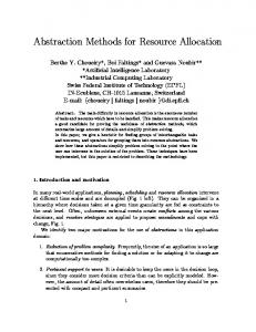
eliminated [5]. For burst mode connection, priority is given to low loss connection for entering the switch in the input queue. Priority is given to the low delay burst mode connection when sending out from the switch. Different queues exist at the output link for low loss burst mode bearer service and low delay burst mode bearer service. We study and compare the following models of the input-output buffer architectures. Case 1
Case 0 Output Case 2
Case 3
Input
Output
Case 5
Case 4
Case 6 CBO traffic Bursty Traffic (Low Delays) Bursty Traffic (Low Loss)
The different buffer architectures examined. Cases 0,1 and 2 consider output queueing only while cases 3-6 consider both the input and the output queues.
g g
g
g
0. There is one common queue at the output port only with equal priority to all bearer services. 1. There are two queues, one for the CBO traffic and one for burst mode traffic (both low loss and low delay) with priority to CBO traffic over burst mode traffic. There is no queueing at the input port. 2. There is a buffer architecture with 3 priority classes in the following priority order, CBO, low delay burst mode and low loss burst mode. There is no queueing at the input port. 3. The buffer architecture consists of an input queue and an output queue. Equal priority is given to all bearer services in both the input and the output queues.
-4-
[Petia Todorova] g
g g
[Resource Allocation in ATM]
4. There are 2 queues, one for the CBO traffic and one for the burst mode traffic (both low loss and low delay) with priority to CBO traffic over burst mode traffic at both the input and the output ports. 5. There are 3 queues at both the input and the output port. The priority order at both the ports is identical to the one mentioned in case 2. 6. Same as case 5, except that low loss bursty traffic is given priority over low delay traffic at the input port, while low delay traffic has higher priority at the output port. CBO traffic has the highest priority at both the input and the output port.
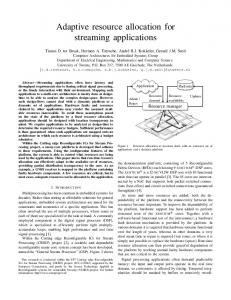
6. Simulation Model We assume in our model that arrivals for each kind of bearer service are Poisson. When a large number of arrivals are multiplexed onto the same link, the arrival process appears to be Poisson. Furthermore, the M/D/1 model for the output queues is robust with respect to the traffic mix and provides generally over-dimensioned buffers. We would like to determine the buffer size which would allow a overflow rate of $10 sup -9 $ or less (this would lead to end to end overflow rate of $10 sup -8$ with about 10 nodes). However, mathematical analysis of complex queueing schemes that we consider is difficult and simulations at the values of $10 sup -9$ are time-consuming. We, therefore, determined the amount of buffer required for an overflow rate of $10 sup -4$ by simulation and extrapolated it to $10 sup -9$, using the fact that at such low values, the tail distribution of any G/G/1 system can be approximated by an exponential. The six different buffer architectures mentioned in the previous sections were compared by means of a simulator developed in CSIM[6]. Different buffer architectures were simulated as variations of an M/D/1 queue i.e. buffer architecture 0 was a simple M/D/1 queue, while buffer architecture 1 was a 2-level M/D/1 queue with priorities. In the cases (architectures 3 4 5 and 6 ) where queueing at both the output and input port was simulated, the service time at the input port was assumed to be one-fifth of the time to transmit a cell at the output port. The simulation model consisted of 5 input pipes and one output pipe(see section 5) were used for the simulation. The simulation results are shown in Figures 1 through 6 below. Figure 1 shows the maximum delay achieved for CBO traffic with different architectures. The maximum delay was defined as the delay that is exceeded by no more than $10 sup -9$ of the cells in the simulation. This delay bound serves as a better index than the average delay, since this determines the amount of buffering required to eliminate the delay fluctuations of the cells on a connection and to provide time-transparency. [ In the figures, the line marked case_0 shows the delays characteristics for architecture 0 , case_1 for architecture 1, and so on]. It can be seen that the separation of CBO traffic from bursty traffic results in substantial improvement af delay characteristics. Our results are consistent with those of Murase et. al. [5]. Figure 2 shows the maximum delays for bursty traffic with low delay requirements. Its maximum delay is slightly worse than CBO traffic, but the separation of the two types of bursty traffic (architectures 2, 5 and 6) results in lower delays for low delay bursty traffic as compared to architectures which do not separate them (architectures 1 or 3). In both these figures, the cell delays are shown as a multiple of the time required to transmit an ATM cell on the output link. For a 53 byte ATM cell, (48 bytes of data + 5
-5-
[Petia Todorova]
[Resource Allocation in ATM]
bytes of header) on a 45 Mbps line, the time to process an ATM cell is roughly 10 $mu s$. Figure 1 tells us that at a switch utilization of 70%, the delay of a CBO cell will not exceed a delay of 270 $mu s$ for a switch using buffer architecture 0 with a probability of $10 sup -9$. We would like to remind the user that the utilization reflects the combined utilization of the output link by all the three traffic types where each of the component traffics contributes to one-third of the total traffic. For the 53 byte ATM cell on a 45Mbps line, 70% utilization consists of a traffic of 31.5 Mbps, of which 10.5 Mbps is CBO, 10.5 Mbps is due to low delay bursty traffic, and 10.5 Mbps is due to low loss bursty traffic. Each of the buffer architectures mentioned above may implement a common shared pool of buffers with appropriate priorities for taking out cells belonging to different traffic types or allocate separate buffers to each of the three types of traffic. Since all ATM cells are of the same size, the total buffer space required in a shared pool architecture remains the same. Such sharing may not be possible due to implementation constraints, or if the switch designer may prefer to insulate one type of traffic from the others. Figure 3, 4 and 5 examine the amount of buffer space required to have a loss probability less than $10 sup -9$ for each of the three traffic types with different buffer architectures. It can be seen that the buffer space required for CBO and low delay burst mode traffic is reduced, while the buffer space required for low loss bursty traffic is much higher. The size of buffers is counted in multiples of ATM cell size, thus at a utilization of 70% with buffer architecture 0, we need a buffer of size 24 * 53 bytes or slightly in excess of 1.3 Kilobytes of buffer space to ensure that the loss probability for low loss bursty traffic is $10 sup -9$ or less (from Figure 5). For the same architecture, Figure 3 tells us that the CBO traffic requires a buffer space of 0.8 Kilobytes while low delay bursty traffic requires a buffer space of 0.95 Kilobytes (from Figure 4). Thus the total amount of buffer space required is about 3 Kilobytes, which can also be seen in Figure 6, which shows the total buffer space required for each of the buffer architectures (with separate buffer pool for each of the three types) and with a shared pool of buffer. The total amount of buffer required with a shared pool is independent of the buffer architecture used. If the traffic types were all sharing a common buffer space, then we would only need a space of about 1.5 Kilobytes. Thus, we save over 50% of the buffer by using a shared pool. Figure 6 shows that the difference in buffer space requirements of different buffer architectures with partitioned buffers is not significant. In the simulations we found that a relatively small buffer at the input port, capable only of holding up to 9 ATM cells is sufficient to ensure a low loss probability in all the different buffer architectures. In summary, the separation of CBO and bursty traffic is to the advantage of CBO traffic, but penalizes bursty traffic with low delay requirements. Separation of the bursty traffic into a two classes (architecture 2) solves this problem. However, there is no significant difference in performance of low loss bursty traffic and low delay bursty traffic, if we switch the input priorities (as seen in Figure 4 and 5) for buffer architectures 5 and 6. Maintaining a shared pool of buffers between the different classes of traffic results in a lower loss rate for the same amount of buffer space(Figure 6). Thus, we recommend buffer architecture 5 or 6 for use in an ATM switch supporting the above-mentioned traffic types, with a shared pool of buffers for all the traffic types.
-6-
[Petia Todorova]
[Resource Allocation in ATM]
7. Conclusions Comparing with the previous works we introduce a common buffer storage allocation architecture, differentiating CBO and burst mode services. We introduce priority schemes corresponding to the real traffic characteristics taking into account all the delay component between end users. We find that a buffer architecture which differentiates between quasi-static traffic and two types of bursty traffic has the best possible performance among all the examined architectures. 8. References [1] J.P.Condruse and M.Servel, "Prelude: an Asynchronous Time-Division Switching Network", Proc. of ICC ’87, June 1987, Seattle, pp 769-773. [2] Y.S.Yeh, M.G.Hlyuchi and A.S.Acompora, "The knockout switch: a simple modular architecture for high-performance packet switching", ISS ’87, March 1987. [3] M.J.Karol, M.G.Hlyuchi and S.P. Morgan, "Input versus output queueing on a space-division packet switch", IEEE Trans. on Commun., COM-35, No 12, Dec. 1987, pp 1347-1356 [4] G.J.Fitzpatrick and E.A.Munter, "Input Buffered ATM switch traffic Performance", Multimedia ’89 Ottawa, April 20-23, 1989 paper 4.2 [5] T.Murase, H.Suzuki, T.Takenchi, "Continuous Bit Stream Oriented Services in ATM network", C&C Sytems Research Laboratoories, NEC Corporation. [6] H. Schwetman, "CSIM Reference Manual (Revision 12)", MCC Tech. Rept. No. ACA-ST-252-87, November 1987.
-7-
[Petia Todorova]
[Resource Allocation in ATM]
Low Delay Bursty Traffic Delay
CBO delay Characteristics
150
units
units 100
case_4 case_1
case_3 case_0 100
case_3 case_0
50 case_5 case_6 case_2
50 Other Cases
0 0.40 0.50 0.60 0.70 0.80 0.90 1.00
0 0.40
Utilization
0.60
0.70
0.80
0.90
Utilization
Figure 1
50
0.50
Figure 2
60
CBO Traffic Buffer Requirement
Low Delay Bursty: Buffer Req. units
units
case_4 case_1
50
40 case_0 case_3
40
case_0 case_3
30 30 20 Other Cases 10
case_2 case_6 case_5
20
10
0 0.40 0.50 0.60 0.70 0.80 0.90 1.00 Utilization
0 0.40 0.50 0.60 0.70 0.80 0.90 1.00 Utilization
Figure 3
Figure 4
-8-
1.00
[Petia Todorova]
100
[Resource Allocation in ATM]
Low loss Bursty Traffic: 150
Buffer Requirement
units
case_2 case_6 case_5
units
Total Buffer Requirement
case 2, 5 , 6 case 0,1,3,4
100
shared case_1 case_4
50
case_0 case_3
50
0 0.40 0.50 0.60 0.70 0.80 0.90 1.00
0 0.40 0.50 0.60 0.70 0.80 0.90 1.00 Utilization
Utilization Figure 6
Figure 5
-9-