our approach achieves 78.5% accuracy on Caltech-101 and. 75.2% on the 102 Flowers dataset when trained on 30 in- stances per class and it achieves 92.7% ...
Robust Classification of Objects, Faces, and Flowers Using Natural Image Statistics Christopher Kanan and Garrison Cottrell Department of Computer Science and Engineering University of California, San Diego {ckanan,gary}@ucsd.edu
Abstract Classification of images in many category datasets has rapidly improved in recent years. However, systems that perform well on particular datasets typically have one or more limitations such as a failure to generalize across visual tasks (e.g., requiring a face detector or extensive retuning of parameters), insufficient translation invariance, inability to cope with partial views and occlusion, or significant performance degradation as the number of classes is increased. Here we attempt to overcome these challenges using a model that combines sequential visual attention using fixations with sparse coding. The model’s biologically-inspired filters are acquired using unsupervised learning applied to natural image patches. Using only a single feature type, our approach achieves 78.5% accuracy on Caltech-101 and 75.2% on the 102 Flowers dataset when trained on 30 instances per class and it achieves 92.7% accuracy on the AR Face database with 1 training instance per person. The same features and parameters are used across these datasets to illustrate its robust performance.
Figure 1. Two images and their corresponding bottom-up saliency maps, which indicate interesting features in an image. Values with high salience are red and low are blue. Saliency maps can be used in object recognition by using them as interest point operators.
1. Introduction
haps inadvertently, have been incorporated into state-of-theart methods in object recognition. For example, the computation of SIFT descriptors [21] begins by using difference of Gaussian (DOG) filters at multiple scales, which is similar to the sort of computation done in the vertebrate retina [10]. Another example is spatial pooling of features or “boxcar filtering” [17, 31, 28, 29, 38], a computation performed by many neurons such as complex cells in primary visual cortex (V1) [31]. Sparse coding algorithms were pioneered in the computational neuroscience community with Independent Component Analysis (ICA) [4, 36] and efficient coding models [7], but it has recently been adopted by the computer vision community [33, 38, 30]. However, one aspect of primate vision that has been
Bestowing an artificial vision system with a fraction of the abilities we primates enjoy has been the goal of many computational vision researchers. While steady progress has been made toward this objective, the gap between the capabilities of the primate visual system and state-of-the-art object recognition systems remains vast. Humans are capable of accurately recognizing thousands of object categories and the primate visual system copes very well with translation, scale, and rotation variance [31]. This has motivated many vision researchers to study human vision in order to extract operating principles that may improve object recognition techniques [31, 24, 28, 29]. Aspects of these biologically inspired approaches, per1
mostly ignored by computer vision researchers is visual attention [13]. Because we cannot process an entire visual scene at once, we sequentially look at, or fixate, salient locations of an object or in a scene. The fixated region is analyzed and then attention is redirected to other salient regions using saccades, ballistic eye movements that are an overt manifestation of attention. We actively move our eyes to direct our highest resolution of visual processing towards interesting things over 170,000 times per day or about 3 saccades per second [32]. Saliency maps are a successful and biologically plausible technique for modeling visual attention (see figure 1). In this paper we propose an approach based upon two facets of the visual system: sparse visual features that capture the statistical regularities in natural scenes and sequential fixation-based visual attention. Our method is empirically validated using large object, face, and flower datasets.
organization of the features and an agent’s current goal [13]. These maps can be entirely stimulus driven, or bottom-up, if the model lacks a specific goal. An example is provided in figure 1. There are numerous areas of the primate brain that contain putative saliency maps such as the frontal eye fields, superior colliculus, and lateral intraparietal sulcus [9]. There are many computational models designed to produce saliency maps. Typically these algorithms produce maps that assign high saliency to regions with rare features or features that differ from their surroundings. What constitutes “rare” varies across the models. One way to represent rare features is to determine how frequently they occur. By fitting a distribution P (F ), where F represents image features, rare features can be immediately found by computing −1 P (F ) for an image. Some of the best models for predicting human eye movements while viewing natural scenes use this approach [39, 3].
2. Background
2.3. Sequential Object Recognition
2.1. Using Natural Image Statistics
While many algorithms for saliency maps have been used to predict the location of human eye movements, little work has been done on how they can be used to recognize individual objects. There are a few notable exceptions [1, 23, 27, 15] and these approaches have several similarities. All of them begin by extracting features across the image along with a saliency map to determine regions of interest. The saliency map may be based on the features used for classification or it may be created using other features. A small window representing a fixation is extracted from the features at the location picked from the saliency map. The extracted fixation is then classified and subsequent fixations are then made according to the saliency map. The mechanisms used to combine information across fixations vary across the models. Besides sharing similar frameworks, these approaches also have implementation similarities. Most of them employ a nonparametric classifier of individual fixations such as k-nearest neighbors or kernel density estimation. The notable exception being Morioka [23] who used a type of discriminative Markov model to represent sequences of fixations with varying length. The types of features they employ vary, ranging from SIFT and luminance [27], Gabor filters [1], a Canny edge detector with a steerable-pyramid [15], and a Harris corner detector [23]. None of these approaches have been evaluated with modern large object datasets such as Caltech-101 [6]. NIMBLE [1], Palletta et al. [27], and Morioka [23] were evaluated using object datasets with static backgrounds containing multiple views of the same object, instead of trying to learn object categories. NIM [15] was evaluated using the AR face dataset (see section 4.2). Here, we adopt the NIMBLE framework [1], while replacing most of its implementation details, such as its fea-
Computer vision has traditionally used features that have been hand-designed, such as Haar wavelets, DOG filters [21, 39], Gabor filters [28, 29, 1], histogram of oriented gradient (HOG) descriptors [25], SIFT descriptors [21, 38, 17, 27], and many others. An alternative is to use Self-taught learning [30]: unsupervised learning applied to unlabeled natural images to learn basis vectors/filters that are good for representing natural images. The training data is generally distinct from the datasets the system will be evaluated on. Self-taught learning works well because it represents natural scenes efficiently, while not overfitting to a particular dataset. The space of possible images is incredibly large. However, natural scenes make up a relatively small portion of this space, so an efficient system should use the statistics of natural scenes to its advantage [7]. In object recognition research self-taught learning algorithms typically do this by employing sparse coding [30, 33]. A sparse code is one in which only a small fraction of the units (binary values, neurons, etc.) are active at any particular time on average [7]. This is in contrast to a local code in which only a single unit is activated to indicate presence or absence or a dense code that represents a signal by having many highly active units. Sparse codes forge a compromise between these two approaches that has yielded many useful algorithms. When sparse coding is applied to natural images, localized, oriented, and bandpass filters are typically learned (see figure 4). These properties are shared by neurons in V1, which exhibit very sparse activity [7].
2.2. Visual Attention A saliency map is a topologically organized map that indicates interesting regions in an image based on the spatial
Figure 2. A high-level overview of the model during classification. See text for details.
tures and saliency map model, with an approach based on natural image statistics. Our system is evaluated using difficult object, face, and flower datasets.
3. Framework & Implementation We first provide a high level description of our model, with the implementation details given in the remainder of this section. To classify an image our approach begins by pre-processing it using mechanisms similar to those in the primate retina to help cope with luminance variation. Sparse ICA features are then extracted from the image. These features are used to compute a saliency map, which is treated as a probability distribution, and locations are randomly sampled from the map. Fixations are extracted from the feature maps at the sampled location, followed by probabilistic classification and the acquisition of additional fixations. A flow chart describing this process is given in figure 2.
3.1. Image Preprocessing Images are first pre-processed to ensure that they are a standard size. This is done by resizing each image such that its smallest dimension is 128 with the other dimension resized accordingly to maintain its aspect ratio. Grayscale images are converted to color. Images are then converted from the default standard RGB (sRGB) color space to LMS color space, which is designed to be similar to the responses of the long-, medium-, and short-wavelength human cones [5]. The minimum value in the LMS image is then subtracted from it, followed by dividing by its maximum value. There is strong biological evidence that luminance adaptation begins in the photoreceptors. They modulate their response to cope with the enormous luminance variance encountered in the natural environment. The logarithm and functions with similar shapes have been used by many computational neuroscientists studying sparse coding as a simple model of the cone’s response to light [7, 4] and they provide a good fit to data from cone photoreceptors. Frequently the use of the logarithm is followed by contrast stretching (or normalization) to ensure the values are between 0 and 1. To model this we apply the following function to the
Figure 3. Before (top row) and after (bottom row) pre-processing images, with three exhibiting altered luminance. The cone nonlinearity helps cope with changes in lighting by preserving important differences while weakening superficial ones.
image’s pixels rnonlinear (z) =
log (�) − log (rlinear (z) + �) , log (�) − log (1 + �)
(1)
where � > 0 is a suitably small value (we use � = 0.05) and rlinear (z) ∈ [0, 1] is a pixel of the image in LMS color space at location z. Note that rnonlinear (z) ∈ [0, 1] as well. See figure 3 for an example of the effects these pre-processing steps have on an image.
3.2. Feature Learning We learn features by applying ICA, a sparse coding algorithm, to image patches from a dataset of unlabeled color natural images. When ICA is used in this way it produces a set of filters with luminance and chromatic properties similar to simple cells in primate visual cortex [37, 4], with the majority of them responding to luminance, similar to the primate magnocellular pathway, and two smaller populations responding to blue/yellow and red/green, similar to the primate koniocellular and parvocellular pathways [19]. To learn ICA filters, we preprocess 584 images from the McGill color image dataset [26]. From each image, 100 b × b × 3 patches are extracted from random locations. The channel mean (L, M, and S) computed across images is subtracted from each patch. Each patch is then treated as a 3b2 dimensional vector. After all patches have been extracted, principal component analysis (PCA) is applied to the patch collection to reduce the dimensionality. We discard the first principal component, which has a very large
used to model each of these unidimensional distributions. The GGD is a flexible distribution which has many common distributions as special cases, such as the Laplace and Gaussian distributions, making it a good choice to model sparse visual features. The GGD is defined as θ i ! fi θi � , (2) P (fi ) = −1 exp − σ 2σi Γ θi i
Figure 4. The learned ICA filters that are applied to images in our approach. When ICA is applied to color image patches it produces a set of features with luminance and chromatic properties similar to that of V1 neurons [37, 4], with the majority of them responding to luminance and two smaller populations responding to yellow/blue and red/green. The same color-opponent organization is found in the Catarrhine primate visual system (i.e., magnocellular, koniocellular, and parvocellular channels).
eigenvalue corresponding to changes in brightness across patches. To limit the number of features learned, we retain d of the remaining principal components, where d is chosen by optimizing performance on an external dataset (see section 3.6). After PCA, we apply Efficient FastICA [14] to the patches. This produces a linear transformation representing image patches as their statistically independent components: Gabor-like edges and bars. The learned filters are shown in figure 4. ICA features are extracted from an m × n × 3 image by filtering it with each of the d ICA filters. The image is padded to ensure the filtered output is the same size as the image. This produces an m × n × d filter response stack, corresponding to a high-dimensional sparse representation of the image.
3.3. Extracting Feature & Saliency Maps We use the Saliency Using Natural statistics (SUN) model to compute bottom-up saliency maps. SUN defines −1 bottom up saliency as P (F ) [39], where F indicates the ICA features. Since the components of F have been made largely statistically independent by ICA, SUN models P (F ) as the Q product of unidimensional distributions: P (F = f ) = i P (fi ), where fi is the i’th element in vector f . The generalized Gaussian distribution (GGD) is
where θi > 0 is the shape parameter, σi > 0 is the scale parameter, and Γ is the gamma function. For each of the d ICA filters, one unidimensional GGD is fit using the patches from section 3.2. The GGD parameters are estimated using the algorithm proposed in [35]. See figure 1 for an example saliency map created using SUN. It is possible to improve the discriminative power of ICA filters by using a GGD fit to their responses [33]. This is done by applying a parametric activation function that weights each dimension of the features according to their 0 statistical frequency. The improved features f are given by � � θi −θ −1 σ , θ γ |f | i i i 0 � , (3) fi = Γ θi−1 where γ denotes the incomplete gamma function and the other terms are those estimated for each of the d GGDs1 . This works by nonlinearly weighting each dimension of f , with rarer responses weighted more heavily.
3.4. Fixations: Spatial Pooling & Whitened PCA The saliency map is normalized to sum to one and then treated as a probability distribution. It is randomly sampled T times. During each fixation t a location `t is chosen according to the saliency map. Centered at location `t we extract a w × w × d stack of filter responses that have had equation 3 applied to them. We let w = 51 in all of our experiments2 . The dimensionality of the patch stack is reduced by spatially subsampling it using a spatial pyramid [17]. Our spatial pyramid divides up each w × w filter response into 1 × 1, 2 × 2, and 4 × 4 grids and the mean filter response is computed in each grid cell. The spatial pyramid levels are concatenated to form a vector, which is normalized to unit length. Across the d stack layers this reduces the dimensionality from w × w × d (i.e., 512 d) to 21d. `t is normalized by the height and width of the image and stored along with the corresponding features. After acquiring T fixations from every training image, PCA is applied to the collected feature vectors. The first 1 In [33] equation 3 was followed by the probit function. In our early experiments we found that this decreased performance slightly while increasing computation time, so we do not use it here.� � 2 The value 51 comes from the equation w = 2 1 s + 1, where s = r 128 is the smallest side of the input image due to the preprocessing steps and r = 5 (chosen arbitrarily).
500 principal components, corresponding to those with the largest eigenvalues, are retained. The retained principal components are then whitened (i.e., normalized according to their eigenvalues to induce isotropic variance). Finally, the post-PCA fixation features, denoted wk,i , are each made unit length.
3.5. Training & Classification Classification is done using the NIMBLE approach [1]. NIMBLE uses kernel density estimation (KDE) to model P (gt |C = k), where gt is the vector of fixation features (i.e., from the procedure described in section 3.4) acquired at time t and k is one of the classes the model has been trained on. The information acquired from fixations 1 to T is combined by assuming fixations are statistically independent (i.e., the Naïve Bayes’ assumption), T � � Y T P (gt |C = k) . P {gt }1 |C = k =
(4)
t=1
This is turned into a classifier using Bayes’ rule, T � � Y T P (gt |C = k) , (5) P C = k| {gt }1 ∝ P (C = k) t=1
where P (C = k) is the class prior. In all of our experiments we assume P (C = k) is uniform and we fix T = 100, which would be about 30 s of viewing time for a person assuming 3 fixations/second. We use 1-nearest neighbor KDE in our implementation of P (gt |C = k). We combine the feature-to-exemplar based distance with a distance based on their difference in normalized (x, y) −location coordinates [2, 15]. This gives us a parameter free estimate of the posterior probability of each class given the fixations acquired from an image: P (gt |C = k) ∝ max
1
, 2 + α kvk,i − `t k2 + � (6) where � > 0 is a small value to ensure P (gt |C = k) is a real number (we use ε = 10−4 ), wk,i is a vector representing the i’th exemplar of a fixation from class k, α = 0.5 is a fixed location “weight” term, vk,i is the normalized (x, y)coordinates at the center of wk,i , and `t is the corresponding location term for gt . After T fixations the class with the greatest posterior is assigned. This approach is simple, requires no tuning of kernel variance, and Barrington et al. [1] found it exhibited greater accuracy than Gaussian KDE. Our implementation performs a simple linear search, since most methods to speed up nearest neighbor tend to provide little benefit in high dimensional spaces. i
kwk,i −
2 gt k2
3.6. Parameter Selection While there are not many “meta-parameters” in our approach, we do need to select the size and number of the image patches/filters. This was done by combining the Butterfly3 [18] and Bird [16] datasets resulting in a dataset with 12 classes that exhibit many of the challenges we wish to overcome. We selected 7 random images per class to train the model and 14 different images per class to test the model. The model that achieved the greatest accuracy was retained. The filter size ranged from 12 to 26 pixels and the number of filters ranged from 122 to 262 . The best parameters were found to be 192 filters of size 24 × 24 pixels. Due to time constraints we had to fix some parameters to reasonable values. For example, the number of principal components was held fixed at 500, we did not tune the size of the fixations, and we fixed the location weight term α to 21 .
4. Experiments & Results For each dataset we perform 5-fold random crossvalidation. Unless otherwise noted, per cross-validation run each class has n randomly selected training images chosen, where n is varied, and up to 30 test images randomly selected (distinct from the training images) unless fewer than 30 are available in which case all of the available images are used. After each run we compute the mean per class accuracy (i.e., the standard procedure for Caltech-101 and Caltech-256). We report the mean accuracy of the runs and we compare against recent state-of-the art results. The raw numbers and standard error values can be found in the supplementary materials.
4.1. Objects The Caltech-101 dataset [6] contains 101 diverse classes (e.g., faces, beavers, anchors, etc.) with a large amount of intra-class appearance and shape variability. Caltech256 [11] is similar to Caltech-101, but it contains 256 classes with even greater intra-class variability and it exhibits location variability. In both cases the images vary in resolution. The NIMBLE framework handles this elegantly, since it only extracts square fixations of f 0 features. Our Caltech-101 results compared with other recent papers [2, 8, 12, 17, 28, 38, 11] are shown in figure 5 and our Caltech-256 results are given in figure 6. Our results are very good compared to other approaches using a single feature type, but they are exceeded when multiple feature types are used. For example, Gehler and Nowozin [8] train a SVM for each of their five feature types and then use boosting to combine the kernels whereas our approach uses a single feature type and a much simpler classifier. 3 We
combine the two Monarch butterfly classes in [18].
Figure 5. Performance of our approach on the Caltech-101 dataset [6] compared to other recent papers [2, 8, 12, 17, 28, 38, 11]. Our performance is comparable to Gehler and Nowozin [8] when they use a combination of five types of features, although we are slightly exceeded by Boiman et al. [2] when they use five feature types. We substantially exceed all of the single feature approaches.
Figure 6. Performance of our approach on the Caltech-256 dataset [11] compared to other recent papers [2, 8, 28, 38, 11].
Figure 8. Performance results from the AR face dataset compared with other recent papers [34, 29, 20]. Our results are very good even when using a single training instance. Note that our approach and Pinto et al. [29] have very similar performance for 5 and 8 training instances.
under varying lighting, expression, and dress conditions (see figure 7). We use images from 120 individuals with 26 images each. We trained our system using 1, 5, and 8 instances per class and tested on the remaining images. To compare our results to Singh et al. [34], for the single training instance case we used the first image for each person in a default pose with uniform lighting and for the 2 and 3 image cases we used the first 3 images per person, which also have uniform lighting and dress. For the 5 and 8 image cases we picked the training images randomly, and tested on all of the remaining images. The performance of our approach appears to be comparable to [28] when we use 5 and 8 training instances, while exceeding Singh et al.’s approach [34], which includes a face detection preprocessing step and was specially designed to handle disguises such as sunglasses. To compare the performance of our model with NIM [15], another fixation-based approach, we trained our model using only the first image from the first 10 classes in AR. After 100 train and test fixations, NIM achieved 92.2% accuracy compared to our 100% accuracy.
4.3. Flowers
Figure 7. Several people from the AR dataset [22] under various lighting, clothing, and facial expression conditions.
4.2. Faces The Aleix and Robert (AR) dataset [22] is a large face dataset containing over 4,000 color face images (768 × 576)
The 102 Flowers dataset consists of 8189 images from 102 flower categories [25]. Several examples are shown in figure 9. Every class has at least 40 images. We train our model using 1, 5, 10, 15, 20, and 30 unsegmented training images per class. Using a segmented version of the dataset with 20 training images per class Nilsback and Zisserman [25] achieved 72.8% accuracy with a combination of HSV descriptors, two types of SIFT descriptors, and a HOG descriptor.
Figure 9. Several examples from the 102 Flowers dataset [25].
can be extremely successful. They largely resolve issues with translation variance and provide a compelling application for saliency maps. We consistently perform well compared to other approaches using few training examples. While we have employed sparse visual features learned from natural image patches, the approach can be readily extended to additional feature types. For many datasets our results using a single feature type are comparable to results using sophisticated methods to combine five different feature types. A video demo and MATLAB source code for our approch are provided at http://www.chriskanan.com/nimble
Acknowledgements We would like to thank Paul Ruvolo, Honghao Shan, and Matus Telgarsky for their feedback and advice. This work was supported by the the James S. McDonnell Foundation (Perceptual Expertise Network, I. Gauthier, PI), and the NSF (grant #SBE-0542013 to the Temporal Dynamics of Learning Center, G.W. Cottrell, PI and IGERT Grant #DGE-0333451 to G.W. Cottrell/V.R. de Sa.).
References
Figure 10. Performance results from the 102 Flowers dataset [25]. Nilsback and Zisserman used segmented images with a combination of four feature types with multiple kernel learning [25]. Our performance on unsegmented images is almost as good as their four feature type system and our performance is substantially better than their best model using a single feature type.
5. Discussion & Conclusions One of the reasons we think our approach works well is because it employs a nonparametric exemplar-based classifier. This yields several immediate benefits: it does not degrade the discriminability of the features [2] and it lets us employ a simple representation of spatial relationships. While our approach requires no training other than PCA once the features are learned, a linear search is suboptimal and there is likely a large amount of duplicate information amongst the stored exemplars. To some extent this could be remedied by employing an algorithm for pruning similar nearest neighbors. We are investigating better ways to make and combine fixations. The Naïve Bayes’ assumption is obviously false and learning a more flexible model (e.g., a Chow-Liu tree) could lead to performance improvements. Using a Markov model to determine where to fixate may also prevent excessive fixations to salient regions that are irrelevant based on the trained classes and recently acquired fixations [27, 23]. Our work demonstrates that fixation-based approaches
[1] L. Barrington, T. K. Marks, J. H.-w. Hsiao, and G. W. Cottrell. NIMBLE: A kernel density model of saccade-based visual memory. Journal of Vision, 8:1– 14, 2008. [2] O. Boiman, E. Shechtman, and M. Irani. In defense of Nearest-Neighbor based image classification. In CVPR 2008, June. [3] N. Bruce and J. Tsotsos. Saliency Based on Information Maximization. In NIPS 2006. [4] M. S. Caywood, B. Willmore, and D. J. Tolhurst. Independent components of color natural scenes resemble V1 neurons in their spatial and color tuning. Journal of Neurophysiology, 91:2859–73, 2004. [5] M. Fairchild. Color appearance models. Wiley Interscience, 2nd edition, 2005. [6] L. Fei-fei, R. Fergus, and P. Perona. Learning generative visual models from few training examples: an incremental bayesian approach tested on 101 object categories. In CVPR 2004. [7] D. Field. What is the goal of sensory coding? Neural Computation, 6:559–601, 1994. [8] P. V. Gehler and S. Nowozin. On Feature Combination for Multiclass Object Classification. In ICCV 2009. [9] P. Glimcher. Making choices: the neurophysiology of visual-saccadic decision making. Trends in Neurosciences, 24:654–659, 2001. [10] D. Graham, D. Chandler, and D. Field. Can the theory of "whitening" explain the center-surround properties
of retinal ganglion cell receptive fields? Vision Research, 46:2901–2913, 2006. [11] G. Griffin, A. Holub, and P. Perona. The Caltech-256. Caltech Technical Report 7694, 2007. [12] C. Gu, J. Lim, P. ArbelŽaez, and J. Malik. Recognition using Regions. In CVPR 2009. [13] L. Itti and C. Koch. Computational Modelling of Visual Attention. Nature Reviews Neurosciece, 2:194– 203, 2001. [14] Z. Koldovský, P. Tichavský, and E. Oja. Efficient Variant Of Algorithm FastICA For Independent Component Analysis Attaining The Cramér-Rao Lower Bound. IEEE Trans. on Neural Networks, 17:1090– 1095, 2006. [15] J. Lacroix, E. Postma, J. Van Den Herik, and J. Murre. Toward a visual cognitive system using active topdown saccadic control. Inernational Journal of Humanoid Robotics, 5, 2008. [16] S. Lazebnik, C. Schmid, and J. Ponce. A Maximum Entropy Framework for Part-Based Texture and Object Recognition. In ICCV 2005. [17] S. Lazebnik, C. Schmid, and J. Ponce. Beyond Bags of Features: Spatial Pyramid Matching for Recognizing Natural Scene Categories. In CVPR 2006. [18] S. Lazebnik, C. Schmid, and J. Ponce. Semi-Local Affine Parts for Object Recognition. In Proc. British Machine Vision Conference 2004. [19] M. Levine. Fundamentals of Sensation and Perception. Oxford University Press, 3rd edition, 2006. [20] Y. Liang, C. Li, W. Gong, and Y. Pan. Uncorrelated linear discriminant analysis based on weighted pairwise Fisher criterion. Pattern Recognition, 40:3606– 3615, 2007. [21] D. Lowe. Distinctive image features from scaleinvariant keypoints. IJCV, 60:91–110, 2004. [22] A. Martinez and R. Benavente. The AR Face Database. CVC Technical Report #24, 1998. [23] N. Morioka. Learning object representations using sequential patterns. In Australasian Conference on Artificial Intelligence 2008. [24] J. Mutch and D. Lowe. Multiclass Object Recognition with Sparse, Localized Features. In CVPR 2006, pages 11–18, 2006. [25] M.-E. Nilsback and A. Zisserman. Automated flower classification over a large number of classes. In Proc. Indian Conference on Computer Vision, Graphics and Image Processing 2008. [26] A. Olmos and F. Kingdom. McGill Calibrated Colour Image Database.
[27] L. Paletta, G. Fritz, and C. Seifert. Q-learning of sequential attention for visual object recognition from informative local descriptors. In ICML 2005. [28] N. Pinto, D. Cox, and J. DiCarlo. Why is Real-World Visual Object Recognition Hard? PLoS Computational Biology, 4, 2008. [29] N. Pinto, J. DiCarlo, and D. Cox. Establishing Good Benchmarks and Baselines for Face Recognition. In ECCV 2008. [30] R. Raina, A. Battle, H. Lee, B. Packer, and A. Ng. Self-taught learning: Transfer learning from unlabeled data. In ICML 2007. [31] M. Riesenhuber and T. Poggio. Hierarchical models of object recognition in cortex. Nature Neuroscience, 2:1019–1025, 1999. [32] P. Schiller. The neural control of visually guided eye movements. Cognitive neuroscience of attention: A developmental perspective, pages 3–50, 1998. [33] H. Shan and G. Cottrell. Looking around the backyard helps to recognize faces and digits. In CVPR 2008. [34] R. Singh, M. Vatsa, and A. Noore. Face Recognition with Disguise and Single Gallery Images. Image and Vision Computing, 27:245–257, 2007. [35] K. Song. A globally convergent and consistent method for estimating the shape parameter of a generalized Gaussian distribution. IEEE Transactions on Information Theory, 52:510–527, 2006. [36] J. Van Hateren and A. Van Der Schaaf. Independent component filters of natural images compared with simple cells in primary visual cortex. Proc R Soc London B., 265:359–366, 1998. [37] T. Wachtler, T. Lee, and T. Sejnowski. Chromatic structure of natural scenes. J. Opt. Soc. Am. A, 18:65– 77, 2001. [38] J. Yang, K. Yu, Y. Gong, and T. Huang. Linear Spatial Pyramid Matching Using Sparse Coding for Image Classification. In CVPR 2009. [39] L. Zhang, M. H. Tong, T. K. Marks, H. Shan, and G. W. Cottrell. SUN: A Bayesian framework for saliency using natural statistics. Journal of Vision, 8:1–20, 2008.