Jul 6, 2017 - ME] 6 Jul 2017 ..... consistently estimated through a plug - in procedure inspired in this expression, by. ÌF(y) = 1 n n. â i=1. {AiI{Yiâ¤y}. ÌÏn(Xi). }.
Robust Doubly Protected Estimators for Quantiles with Missing Data. Julieta Molina(1) , Mariela Sued(2) , Marina Valdora(1) , V´ıctor Yohai(2) (1) Universidad de Buenos Aires, (2) Universidad de Buenos Aires and Conicet.
arXiv:1707.01951v1 [stat.ME] 6 Jul 2017
July 10, 2017 Abstract Doubly protected estimators are widely used for estimating the population mean of an outcome Y from a sample where the response is missing in some individuals. To compensate for the missing responses, a vector X of covariates is observed at each individual, and the missing mechanism is assumed to be independent of the response, conditioned on X (missing at random). In recent years, many authors have moved from the mean to the median, and more generally, doubly protected estimators of the quantiles have been proposed, assuming a parametric regression model for the relationship between X and Y and a parametric form for the propensity score. In this work, we present doubly protected estimators for the quantiles that are also robust, in the sense that they are resistant to the presence of outliers in the sample. We also flexibilize the model for the relationship between X and Y . Thus we present robust doubly protected estimators for the quantiles of the response in the presence of missing observations, postulating a semiparametric regression model for the relationship between the response and the covariates and a parametric model for the propensity score.
Keywords: missing data, quantile estimation, doubly protected estimator, robust estimator, semiparametric regression model.
1
Introduction
The problem of estimating the mean of a random variable Y from an incomplete data set under the missing at random (MAR) assumption has attracted the attention of the statistical community during the last decades. MAR establishes that the variable of interest Y and the response indicator A are conditionally independent given an always observed vector X of covariates. Most of the existing proposals are based on three different approaches : inverse probability weighted (IPW), outcome regression (OR) and doubly protected (DP) methods. Inverse probability weighted methods are based on the estimation of the propensity score, denoted by π(X), which is defined as the response probability given X. The estimators obtained using this methodology are, essentially, weighted means of observed responses. The weights are determined as the inverse of the estimated propensity scores and their aim is to compensate for the missing observations. Different apporaches have been considered for the estimation of the 1
propensity score used in the construction of IPW estimators, for example, logistic regression models [1, 2] and splines [3]. Outcome regression methods require the estimation of the regression function of Y given X. The estimators for E(Y ) built by these techniques average predicted values computed using the estimated regression function g(X) = E(Y | X). Methods to estimate the regression function g(X) include linear regression [4], kernel smoothing [5], semiparametric estimation [7, 8] and local polynomials [9]. IPW procedures are consistent for E(Y ) whenever the propensity score is properly estimated. For instance, in the parametric setting, this requires a correctly specified model for π(X). Similarly, OR estimators are consistent provided the predicted values are based on a consistent estimation of the regression function. In a parametric framework, this means that the postulated model for the regression function g(X) should be correct. Doubly protected estimators, also known as doubly robust, combine IPW and OR methods providing consistent estimators for E(Y ) when either the model for the propensity score or the model for the regression function is correct, without having to specify in advance which of them holds. Thus, we get consistent estimators in the union of both the model for the propensity and the model for the regression function. In-depth analysis and examples of doubly protected methods are given in [2],[10], [11], [12], and [13]. Besides the estimation of E(Y ), many authors have begun to apply these methods to the estimation of the quantiles of the distribution of Y in the described MAR context. Many of them use the available techniques just described to estimate the distribution function F0 of Y with Fbn . Then, the quantiles of Fbn are used to estimate those of F0 . Cheng and Chu [14], proposed a Nadaraya-Watson estimator for the conditional distribution of Y given X and use it to derive a non parametric estimator for the distribution function F0 . Yang, Kim and Shin [15] presented an imputation method for estimating the quantiles. Imputed data sets are constructed generating plausible values to represent the uncertainty about missing responses. The final quantile estimator is obtained combining those computed at each of the multiply imputed data sets. Wang and Qin ([16]) proposed to estimate F0 using IPW techniques but estimating the propensity score via kernel regression. D´ıaz I. [17] proposed to estimate F0 under a semiparametric model, using doubly protected techniques by targeted maximum likelihood procedures. Besides the estimation of the quantiles of F0 , other location parameters have been considered and most of them also deal with the presence of outliers in the sample, providing robust methods for estimating the parameter of interest. For instance, Bianco et al. [18] used IPW techniques, imputing non parametric estimators of the propensity score π(X), and also regression procedures under a semiparametric partially linear regression model to construct location estimators. Asymptotic properties of the estimators involved in these proposals are presented in Bianco et al. [19]. Sued and Yohai [20] also deal with the estimation of the entire distribution of Y considering a semiparametric regression model. Predicted values are combined with observed residuals to emulate a complete data set, based on which one can compute any desired estimator. A robust fit of the regression model is used to take care of anomalous observations. This proposal consistently estimates any parameter defined through a weakly continuous functional at the response’s distribution.
2
Causal inference is an area where missing data inevitably occur because of the definition of counterfactual variables. A large amount of procedures have been designed in such a framework. Among them, we can cite the work by Lunceford and Davidian [10] and the work by Zhang et al. [21] on quantile estimation. Lunceford and Davidian proposed modified IPW estimators in the causal setting, achieving a higher precision compared to the classical ones. Zhang et al. presented several proposals for estimating the distribution function F0 , all of them based on parametric models for the propensity score or for the conditional distribution of Y given X. They also constructed doubly protected estimators for F0 and, therefore, for the quantiles. No protection is provided against the effect of outliers, while the regression framework is entirely parametric. All the doubly protected proposals to estimate the distribution function F0 when Y is missing in some individuals considered up to now are very sensitive to anomalous observations. This is due to the fact that they are based on least squares fits and/or in standard maximum likelihood techniques. In this work, we introduce resistant doubly protected estimators for the distribution function of a scalar outcome that is missing by happenstance on some individuals under a parametric model for the propensity score and a semiparametric regression model for the relation between the outcome and the covariates, assuming missing at random responses. The paper is organized as follows. Section 2 introduces the classical procedures to estimate the mean of an outcome Y missing at random. In Section 3 we adapt these procedures to the estimation of the distribution function of Y. In order to assess the performance of our estimating procedure, in Section 4 we present the results of a Monte Carlo simulation study.
2 2.1
Classical estimators in missing data. Inverse probability weighted estimators.
We are interested in estimating µ = E(Y ) based on a sample where Y is missing by happenstance on some subjects. To compensate for the missing responses, a vector of covariates X ∈ Rp is available for each individual. Moreover, we assume that data are missing at random (MAR) [22]. MAR establishes that the missing mechanism is not related to the response of interest and it is only related to the observed vector of covariates. To give a formal definition, let A be the indicator of whether or not Y is missing, i.e., A = 1 if Y is observed, and A = 0 when Y is missing. Mathematically, MAR establishes that P(A = 1 | X, Y ) = P(A = 1 | X) = π(X).
(1)
π(X) is known in the literature as the propensity score [23]. In this scenario, E(Y ) can be represented in terms of the distribution of the observed data as E(Y ) = E {AY /π(X)}. This representation leads us to estimate µ by the so-called Horvitz and Thompson method [24], � � AY µ ˆ(ˆ π ) = Pn , (2) π ˆ (X) where π ˆn (X) Pis a consistent estimator of π(X), and Pn is the empirical mean operator, i.e. Pn V = n−1 ni=1 Vi . Notice that the observed responses are weighted according to the inverse 3
of the estimated probability of A = 1 given X, justifying the appellative “inverse probability weighted” (IPW) for such procedures. Moreover, those observed responses corresponding to low values of the estimated propensity score are highly weighted since they should compensate for the high missing rate associated to such a level of covariates. For more details see [25]. Different proposals to estimate π(X) give rise to diverse estimators of E(Y ), according to (2). Nonparametric estimators of the propensity score have been considered by Little and An [3] and, in a causal context, by Hirano, Imbens and Ridder [26]. In order to assume MAR, the vector X is typically high dimensional, and therefore, in practice, non parametrical estimation of the propensity score is infeasible because of the socalled curse of dimensionality (see [27]). For this reason the propensity score is often estimated postulating a parametric working model, assuming that π(X) = π(X; γ 0 ),
(3)
where γ 0 ∈ Rq is an unknown q-dimensional parameter and π(·; ·) : Rp × Rq → [0, 1] is a known function. The maximum-likelihood (ML) estimator of γ 0 can be obtained from (X1 , A1 ), . . . , (Xn , An ), b n . Then, we can estimate π(X) by π b n ). and will be denoted by γ bn (X) := π(X; γ Generalized linear models (GLM) are very popular in this setting. These models postulate that π(X; γ 0 ) = φ(γ T0 X), (4) where φ is a strictly increasing cumulative distribution function. In particular, the linear logistic regression model for the propensity score is obtained by choosing φ(u) = exp(u)/{1 + exp(u)} in (4) (see [2] ).
2.2
Outcome regression estimators.
To construct IPW estimators, we model the relation between the missing mechanism and the covariates and we do not make assumptions on the relation between the outcome and the covariates. To construct regression estimators for E(Y ), we estimate the regression function of Y on X and average predicted values. More precisely, under the missing at random assumption we have that Y | X ∼ Y | (X, A = 1) and therefore the regression function g(X) = E (Y | X) satisfies g(X) = E (Y | X, A = 1). In this way we arrive at a second representation for E(Y ) based on the observed data through the regression function: E(Y ) = E{g(X)}. This alternative characterization for E(Y ) invites us to estimate it by averaging predicted values, with µ b(b gn ) = Pn {b gn (X)} ,
(5)
where gbn (X) is any consistent estimator of g(X). Different ways to estimate g(X) result in different estimators according to (5). A non parametric proposal for gbn (X) is given in Cheng [5], using kernel regression estimation duly adapted to the missing data context, in order to estimate the regression function. Imbens Newey and Ridder [6] proposed non parametric estimation for both the propensity score and the regression function.
4
In practice, working parametric models are postulated for the regression function to overcome the curse of dimensionality, which is a serious obstacle for non parametric methods (see [27]). A parametric model for the regression function assumes that g(X) = g(X; β 0 ),
(6)
where g(·; ·) is a known function and β 0 ∈ Rr is unknown. The unknown parameter β 0 of the b , using the units with observed responses working regression model (6) can be estimated by β n b ) Y by, for instance, the least squares method. Then, g(X) is estimated with gbn (X) := g(X; β n and this expression is imputed in (5) to obtain parametric regression estimators of E(Y ). Kang and Shafer [2] review the regression estimator of µ that results from considering a linear model for the regression function: g(X; β 0 ) = β T0 X. A comprehensive overview of parametric regression estimators is given in [1]. We also want to mention that another way to deal with the curse of dimensionality is to consider intermediate structures like additive models or semiparametric models for the regression function. See, for example, [7] and [28].
2.3
Doubly protected estimators.
Estimators based on inverse probability weighting, as presented in (2) are consistent for µ as far as the propensity score π(X) is consistently estimated. This approach leads to a well specified model for π(X) in the parametric case. On the other hand, regression estimators, as presented in (5), are consistent when the regression function is properly estimated and thus, the regression model is assumed to be correctly specified. To sum up, each procedure forces us to choose in advance what to model in order to decide which estimator should be used to consistently estimate E(Y ). Typically no one knows which model is more suitable, generating a debate on which approach should be used. To end this controversy, estimators which are consistent for E(Y ) whenever, at least, one of the two models is correct were proposed. Such estimators confer more protection to model misspecification than IPW or OR estimators, which are consistent only when the corresponding assumed model holds. Since these estimators are consistent for E(Y ) as long as one of the models succeeds, they are called doubly protected estimators. Doubly protected estimators were discovered by Robins et al. [30, 8], while studying augmented IPW estimators (AIPW). Some years later, Scharfstein et al. [31] showed that some AIPW estimators have the double protection property. To motivate these estimators, they obtained the following expression for the mean that holds assuming MAR and that either p(X) = P(A = 1 | X) or r(X) = E(Y | X) hold: � � �� � � AY A µ=E −E − 1 r(X) . (7) p(X) p(X) Therefore, to obtain doubly protected estimators, we postulate parametric models π(X; γ) =
5
P(A = 1 | X) and g(X; β) = E(Y | X), like in (3) and (6), respectively, and estimate µ by �� � � � � A AY b − Pn µ bDP = Pn − 1 g(X; β n ) , bn) bn) π(X; γ π(X; γ
(8)
b are consistent estimators of γ and β . b n and β where γ n 0 0 The estimator defined in (8) is doubly protected, and also achieves full efficiency in the AIPW class if the model for the propensity and the model for the regression function are both well specified (see [30] and [8]). An in-depth analysis and examples of doubly-protected methods are given in [10], [11], [12] and [2]. For the complete and detailed mathematical theory underlying double protection methodology see [32] and [13].
3
Estimating percentiles of the distribution of Y
In this section, we move from the estimation of E(Y ) to the estimation of the median of the distribution of Y . More generally, in this section, we will focus on the estimation of any quantile of F0 , the distribution of Y . The p-quantile of a distribution F is defined as Tp (F ) = inf{x : F (x) ≥ p}.
(9)
When p = 0.5, we get T0.5 (F ), the median of F . The representation of the p-quantile given in (9) suggests that it can be estimated by Tp (Fbn ), provided Fbn approximates F0 . So, to estimate a p-quantile � of a distribution of Y it is enough to estimate F0 . Note that F0 (y) = P(Y ≤ y) = E I{Y ≤y} . Thus, in the next sections, we will provide different proposals of estimation of the distribution function of Y , mimicking each of the estimators considered in the previous sections, but to estimate now E (`y (Y )), where `y (Y ) = I(Y ≤y) , in lieu of µ = E(Y ).
3.1
IPW estimators of F0 .
Under MAR assumption �
F0 (y) = E I(Y ≤y) = E
�
AI{Y ≤y} π(X)
� ,
(10)
and so, if we apply the procedure developed in Section 2.1, we arrive at the following estimator for F0 (y) � � AI(Y ≤y) FbIPW (y) = Pn , (11) π bn (X) where π b(X) is a consistent estimator of the propensity score. A slightly modified version of this estimator, with weights adding up to one, has already been introduced by Bianco et al. [18] and used for estimating any M-location functional of the distribution of Y . Fbipw was also proposed by Zhang et al. [21] for estimating quantiles under a parametric model for the propensity score.
6
3.2
Regression Estimators of F0
Regression estimators are constructed based on the following representation F0 (y) = E{P(Y ≤ y | X)}.
(12)
Thus, we can estimate F0 with n
X b ≤ y | Xi ). b ≤ y | X) = 1 P(Y FbREG (y) = Pn P(Y n
(13)
i=1
Suppose, for instance, that a generalized linear model is postulated, assuming that Y | X ∼ Gβ0 t X , where {Gθ : θ ∈ Θ} is an exponential family of univariate distributions, and θ is the vector of natural parameters. In this case, because of the MAR assumption, Y | (X, A = 1) ∼ b , the maximum likelihood estimator under Gβt0 X and so β 0 can be consistently estimated with β n the model using the pairs (Xi , Yi ) with Ai = 1. Then, according to (13), in this particular case, we estimate F0 with n 1X b FGLM (y) = (14) Gβb t X (y). n i n i=1
Assume now that Y follows a regression model of the form Y = g(X) + u,
(15)
where g is the unknown regression function that maps Rp into R, and u is independent of X. Moreover, to guarantee the MAR assumption we require that (X, A) is independent of u. Let gbn (X) be a consistent estimator of the regression function, constructed using the pairs (Xi , Yi ) with observed responses (Ai = 1). Under the regression model (15), the assumed independence between u and X implies that P(Y ≤ y | X) = P{u ≤ y − g(X)} and so, it can be estimated with the empirical distribution of the residuals u bj = Yj − gbn (Xj ), for Aj = 1, at y − gbn (X): n
1 X ˆ P(Y ≤ y | X) = Fberror (y − gbn (X)) = Aj I{buj ≤y−bgn (X)} , m
(16)
j=1
where m denotes the number of observed responses, that is m = (13) we obtain the following estimator for F0
Pn
j=1 Aj .
Combining (16) with
n n 1Xb 1 X b F (y) = Ferror (y − gbn (Xi )) = Aj I{buj ≤y−bgn (Xi )} . n nm i=1
(17)
i,j=1
Note that Fˆ asssigns mass 1/(nm) to the values 1 ≤ j ≤ n, Aj = 1,
Ybij = gbn (Xi ) + u bj ,
(18)
where predicted values gbn (Xi ) are combined with residuals u bj to emulate a pseudo-sample of responses Yˆij , as suggested by equation (15). 7
Sued and Yohai [20], proposed a semiparametric regression model for (15), where the regression function is assumed to be in a parametric family: g(X) = g(X; β 0 ), with β 0 ∈ B ⊂ Rq , and g : Rp × B → R is a known function. No other than a centrality condition, namely symmetry around zero, is imposed on the error term u. In fact, Sued and Yohai [20] showed that the centrality condition can be avoided, redefining properly the intercept in the regression model. But, to keep this presentation more accessible, we invite the reader to focus the centered error case. This gives rise to the estimator FˆSY , defined as n 1 X FbSY (y) = Ai I{Ybij ≤y} , nm
(19)
i,j=1
b ). The authors proved that FbSY converges to with Ybij defined as in (18) taking gbn (X) = g(X, β n b F0 , as far as β n converges to β0 . In particular, they considered robust procedures for estimating the regression parameter β 0 , and showed that T (FbSY ) gives rise to a robust method for estimating T (F0 ), for any weak- continuos functional T at F0 . In particular, this procedure allows the estimation of the p-quantiles of F0 with Tp (FbSY ), where Tp is defined in (9). Model (15) with a linear regression function g(X; β 0 ) = β to X and Gaussian errors (u ∼ N (0, σ 2 ) fits the GLM framework described at the beginning of this section. In particular, according to (14), we arrive at the following estimator of F0 ! n X b t Xi y − β 1 n Φ FbG (y) = , (20) n σ b i=1
where Φ denotes the cumulative distribution of a standard normal random variable. This estimator was studied by Zhang et al. in [21]. We remark the semiparametric nature of the estimator FˆSY presented in [20], where no model is assumed for the distribution of the error term u.
3.3
Doubly protected estimator of F0
Replacing Y with I{Y ≤y} in (7), we obtain � � �� � � � AI{Y ≤y} A F0 (y) = E I{Y ≤y} = E −E − 1 ry (X) , p(X) p(X)
(21)
under MAR and supposing either p(X) = P(A = 1 | X) or ry (X) = P(Y ≤ y | X) holds. Assuming π(X) = P(A = 1 | X) and gy (X) = P(Y ≤ y | X), F0 can be doubly protected consistently estimated through a plug - in procedure inspired in this expression, by � � � n � n �� 1 X Ai I{Yi ≤y} 1X Ai b − − 1 gby (Xi ) . F (y) = n π bn (Xi ) n π bn (Xi ) i=1
i=1
At this point, we turn to a parametric model for the propensity score π(X) = π(X; γ 0 ), as in (3), and also assume that the regression function g(X) in model (15) satisfies g(X) = g(X; β 0 ). Thus, we can deal with a semiparametic regression model, instead of a parametric one, where 8
typically also the distribution of the error term is assumed to belong to a parametric family. In this way, using Fberror defined in (16), we arrive at the following semiparametric doubly protected estimator for F0 n
1X FbDP-S (y) = n i=1
�
Ai I{Yi ≤y} bn) π(Xi , γ
�
� � n �� 1 X Ai − − 1 Aj I{g(βb ,Xi )+buj ≤y} , n bn) mn π(Xi , γ
(22)
i,j=1
b are consistent estimators of γ and β . b n and β where γ n 0 0 If a generalized linear model is assumed for Y | X, as decribed in Section 3.2, we obtain the following parametric doubly protected estimator of F0 � � � n � n �� 1 X Ai I{Yi ≤y} 1X Ai FbDP-P (y) = − − 1 Gβb Xi (y) . (23) n bn) bn) n π(Xi , γ n π(Xi , γ i=1
3.4
i=1
Robustness
Atypical observations, called outliers, are common in many real datasets. Classical procedures do not contemplate their existence and therefore their application may lead to wrong conclusions. For instance, the sample mean or the least-squares fit of a regression model, can be very adversely influenced by outliers, even by a single one. Robust methods arise to cope with these atypical observations, mitigating their impact in the final analysis. The median is, probably, the most popular example of a robust procedure to summarize a univariate dataset. More generally, Mlocation estimators have been developed for such a purpose: a robust location summary of a univariate data set. Thus, moving from the estimation of E(Y ) to that of the median of F0 represents a first step in the path towards robustification. However, the methods presented in the previous section, also require regression fits, both to estimate the propensity score and the regression function. In this work we propose to consider a robust alternative for the regression fit of the postulated model that relates X and Y . In fact, when model (6) is combined with a parametric regression function assuming that g(X) = g(X, β 0 ), the least-squares fit will be replaced by a robust one. One way to achieve this robustification is to replace the square loss function by a function ρ satisfying i) ρ is even, ii) ρ is bounded and iii) ρ is increasing in (0, +∞). This is the case of M-estimators, both for location and regression problems. In particular, MMestimators, introduced by Yohai [33] for the linear model and extended to the non linear case in Fasano et al. [34], combines the highest possible tolerance to the presence of outliers, measured by the breakdown point, with an arbitrarily high efficiency in the case of Gaussian errors. R , which denotes Thus, to get a robust doubly protected estimation of F0 , we will now use FˆDP-S b the estimator presented in (22), but constructed with an MM-estimator β n for the regression parameter under model g(X) = g(X; β 0 ). Finally, also the parametric doubly protect estimator presented in Zhang may be robustified, through a robust fit of the generalized linear model postulated for the conditional distribution R , defined as in (14) but with β b obtained again from a robust of Y given X, giving rise to FˆDP-P n fit. 9
The next step is, naturally, to robustify the estimation of γ 0 , the parameter involved in the propensity score. However, this simple approach would not robustify the final estimator. On the contrary, in the presence of outliers in the covariates, extreme values of π b are more likely to appear if γ 0 is estimated robustly than otherwise. Resistance to outliers in A seems a difficult problem, whose solution we are still working on and might be the subject of further work.
4
Monte Carlo Study
In this section we report the results of a Monte Carlo study we made in order to study the performance of the different estimators of the median proposed in this work, as compared to some of the estimators that already existed in the literature. We consider different distributions of the error term u, namely standard normal and student distribution with one and three degrees of freedom. We also investigate the robustness of the proposed estimators, by contaminating the samples with 10% of outliers. The samples considered consist of n i.i.d. random vectors with the same distribution as (X, A, Y ) where X = (X1 , X2 ) is a bivariate standard nomal random vector of covariates, that is, X ∼ N (0, I), A is a binary variable following a Bernoulli distribution with P (A = 1|X) = π(X) = expit((1, X1 , X2 )0 γ 0 ), expit(t) = et /(1 + et ) and γ 0 = (0, 0.1, −1.1) and Y is an outcome generated as Y = β 00 X + u, where β 0 = (−3, 2) and U is independent of (X, A). We consider four different situations: 1. the model for the propensity is well specified and the model for the regression function is well specified. That is, when we adjust for the missing mechanism we fit a logistic regression model with covariates X1 and X2 and when we adjust for the regression function we fit a linear regression model with covariates X1 and X2 . 2. the model for the propensity is well specified and the model for the regression function is misspecified. More precisely, we fit an incorrect model for the regression function, using just the covariate X1 , omitting the covariate X2 . 3. the model for the propensity is misspecified and the model for the regression function is well specified. The misspecification consists in fitting a logistic regression model with only the covariate X1 , omitting the covariate X2 . 4. the model for the propensity is misspecified and the model for the regression functions is misspecified. In each case, we generate N rep = 1000 samples of size n = 100 and we compute 5 different estimators of η = med(Y ): 10
1. ηˆIPW = T0.5 (FˆIPW ) 2. ηˆSY = T0.5 (FˆSY ) 3. ηˆDP-P = T0.5 (FˆDP-P ) R R ) 4. ηˆDP-P = T0.5 (FˆDP-P R R ) 5. ηˆDP-S = T0.5 (FˆDP-S
To recall the definitions of the different estimators of F0 see (11), (19), (23) and the end of Section 3.4. In order to investigate the robustness of the estimators, we consider samples generated with normal errors and we replace 10% of the observations by outliers (X0 , A0 , Y0 ) where • X0 = (2, 0), • P(A0 = 1|X = X0 ) = expit((1, 2, 0)0 γ 0 ), • Y0 ∈ {−100, −90, . . . , −20, −10, 0, 10, 20, . . . , 90, 100}. The contamination scheme is the same as in [20]. Simulation results are summarized in Table 1 and in Figures 1 to 3. In these the five estimating methods considered are labelled IPW, SY, DP-P, DP-P-ROB and DP-S-ROB respectively. These results show that, even though the median is already robust, the estimation of the regression coefficients by a robust method improves the performance of the estimators. This improvement is very important if the sample is contaminated with outliers but it is also noticeable when the sample has a heavy tailed distribution such as a Student or a Cauchy distribution. On the other hand, DP-S-ROB gives better results than DP-P-ROB when the errors follow a Student or Cauchy distribution. This is due to the fact that the latter assumes normal errors while former does not. Table 1 also shows the double robustness of DP-P, DP-P-ROB and DP-S-ROB. In figures 1 to 3 we plot the mean square errors of the different doubly protected estimators as a function of the value of the outlying outcome y0 . These figures show that much robustness is gained by estimating the regression coefficients robustly, using an MM-estimator, instead of using the least squares estimator. Both doubly protected robust estimators give similar results in contaminated samples.
References [1] Little RJ, Rubin DB. Statistical Analysis with Missing Data. John Wiley and Sons 1987. [2] Kang JD, Schafer JL. Demystifying double robustness: A comparison of alternative strategies for estimating a population mean from incomplete data. Statistical science 2007; 523539. [3] Little R, An H. Robust likelihood-based analysis of multivariate data with missing values. Statistica Sinica 2004; 949-968. 11
Empirical MSE when PS and OR models are correct
0.0
0.2
0.4
MSE
0.6
0.8
1.0
DP−S−ROB DP−P DP−P−ROB
−100
−50
0
50
100
y0
Figure 1: Doubly robust estimators in contaminated samples Empirical MSE when PS is correct and OR is incorrect
0.6 0.0
0.2
0.4
MSE
0.8
1.0
DP−S−ROB DP−P DP−P−ROB
−100
−50
0
50
100
y0
Figure 2: Doubly robust estimators in contaminated samples 12
Empirical MSE when PS is incorrect and OR is correct
1.5 0.0
0.5
1.0
MSE
2.0
2.5
DP−S−ROB DP−P DP−P−ROB
−100
−50
0
50
100
y0
Figure 3: Doubly robust estimators in contaminated samples [4] Yates, F. The analysis of replicated experiments when the field results are incomplete. Emp. J. Exp. Agric. 1933; 1, 129-142. [5] Cheng, PE. Nonparametric estimation of mean functionals with data missing at random. Journal of the American Statistical Association 1994; 89, 81-87 [6] Imbens, G. W., Newey, W. K. and Ridder, G. . Mean-square-error calculations for average treatment effects. 2005 [7] Wang Q, Linton O and Hardle W. Semiparametric regression analysis with missing response at random. Journal of the American Statistical Association 2004; 99, 334–345. [8] Robins JM, Rotnitzky A, Zhao LP. Analysis of semiparametric regression models for repeated outcomes in the presence of missing data. Journal of the American Statistical Association 1995; 90(429): 106-121. [9] Gonz´alez–Manteiga, W. and P´erez–Gonz´alez, A. Nonparametric mean estimation with missing data. Comm. Statist. Theory Methods 2004; 33, 277-303. [10] Lunceford JK, Davidian M. Stratification and weighting via the propensity score in estimation of causal treatment effects: a comparative study. Statistics in medicine 2004; 23 (19): 2937-2960.
13
IPW IPW SY SY DP-S-ROB DP-S-ROB DP-S-ROB DP-S-ROB DP-P DP-P DP-P DP-P DP-P-ROB DP-P-ROB DP-P-ROB DP-P-ROB
PS correct incorrect
correct incorrect correct incorrect correct incorrect correct incorrect correct incorrect correct incorrect
OR
correct incorrect correct correct incorrect incorrect correct correct incorrect incorrect correct correct incorrect incorrect
Normal errors 0.381 1.125 0.206 0.945 0.313 0.280 0.683 0.983 0.310 0.268 0.712 0.982 0.310 0.278 0.682 0.976
t3 errors 0.424 1.137 0.233 1.035 0.361 0.310 0.528 1.115 0.361 0.326 0.570 1.104 0.364 0.302 0.537 1.088
Cauchy errors 0.689 1.22 0.339 0.996 0.548 0.469 0.841 1.100 0.707 0.740 0.733 1.063 0.590 0.483 0.942 1.088
Max MSE 0.885 2.300 1.641 4.301 0.675 0.907 0.733 2.355 1.036 1.131 2.706 2.314 0.695 0.945 0.681 2.314
Table 1: M ean square errors of the estimators in different situations. [11] Carpenter J, Kenward, M and Vansteelandt, S. A comparison of multiple imputation and doubly robust estimation for analyses with missing data. Journal of the Royal Statistical Society. 2006; 169, 571-584. [12] Bang H, Robins J. (2005). Doubly Robust Estimation in Missing Data and Causal Inference Models. Biometrics. 2005; 61, 962-972. [13] Van der Laan, M. J. and Robins, J. M. Unified Methods for Censored Longitudinal Data and Causality. 2003; New York. Springer-Verlag. [14] Cheng, P. E., Chu, C. K. Kernel estimation of distribution functions and quantiles with missing data. Statistica Sinica. 1996; 63-78. [15] Yang, S., Kim, J. K., and Shin, D. W. Imputation methods for quantile estimation under missing at random. Statistics and Its Interface. 2013; 6 (3), 369-377. [16] Qihua Wang and Yongsong Qin. Empirical likelihood confidence bands for distribution functions with missing responses. Journal of Statistical Planning and Inference. 2010; 140(9): 27782789. [17] D´ıaz, I.. Efficient estimation of quantiles in missing data models. Journal of Statistical Planning and Inference. 2017 [18] Bianco, A., Boente, G., Gonz´ alez-Manteiga, W., and P´erez-Gonz´alez, A. Estimation of the marginal location under a partially linear model with missing responses. Computational Statistics & Data Analysis. 2010; 54(2), 546-564. 14
[19] Bianco, A, Boente, G, Gonz´ alez-Manteiga, W and Perez Gonzalez, Ana. Asymptotic behaviour of robust estimators in partially linear models with missing responses:The effect of estimating the missing probability on the simplified marginal estimators. Test. 2011; 20 (3), 524-548. [20] Sued M. and Yohai, V. Robust location estimation with missing data. Canadian Journal of Statistics. 2013; 41(1), 111-132. [21] Zhang, Z., Chen, Z., Troendle, J. F. and Zhang, J. Causal inference on quantiles with an obstetric application. Biometrics. 2012; 68(3), 697-706. [22] Rubin DB. Inference and missing data. Biometrika 1976; 63 (3): 581–592. [23] Rosenbaum PR, Rubin DB. The central role of the propensity score in observational studies for causal effects. Biometrika 1983; 41-55. [24] Horvitz DG, Thompson DJ. A generalization of sampling without replacement from a finite universe. Journal of the American statistical Association 1952; 47(260): 663-685. [25] Robins JM, Rotnitzky A. Recovery of information and adjustment for dependent censoring using surrogate markers. Aids Epidemiology. Springer 1992; 297-331 [26] Hirano K, Imbens GW, Ridder G. Efficient estimation of average treatment effects using the estimated propensity score. Econometrica 2003; 71(4): 1161-1189. [27] Stone, C.J. Optimal rates of convergence for nonparametric estimators. Annals of Statistics 1980; 8, 1348-1360. [28] Hastie T.J, Tibshirani RJ. Generalized Additive Models. Chapman and Hall 1990. [29] Healy, M.J.R. and Westmacott,M. Missing values in experiments analyzed on automatic computers. Appl. Statist 1956. [30] Robins JM, Rotnitzky A, Zhao LP. Estimation of regression coefficients when some regressors are not always observed. Journal of the American statistical Association 1994; 89(427): 846-866. [31] Scharfstein D, Rotnitzky a and Robins J. Adjusting for nonignorable drop-Out using semiparametric nonresponse Models. Journal of the American Statistical Association. 1999; 94, 448-499. [32] Robins J and Rotnitzky A. Comment on the Bickel and Kwon article “ Inference for semiparametric models: Some questions and an answer”. Statistica Sinica. 2001; 11, 920-936. [33] Yohai, V. J. High breakdown-point and high efficiency robust estimates for regression; The Annals of Statistics. 1987; 642-656. [34] Fasano M V., Maronna, R. A. Consistency of M estimates for separable nonlinear regression models. 2012; arXiv preprint arXiv:1207.0473. 15
[35] Rosner B. Fundamentals of Biostatistics, 5th ed., Pacific Grove, CA: Duxbury 1999. [36] Niu X, Hoff P. covreg: A simultaneous regression model for the mean and covariance. R package version 2014. [37] Neyman J. Sur les applications de la th´eorie des probabilit´es aux experiences agricoles: Essai des principes. Roczniki Nauk Rolniczych 1923; 10: 1-51. [38] Rubin DB. Estimating causal effects of treatments in randomized and nonrandomized studies. Journal of educational Psychology 1974; 66(5): 688.
16