5 illustrates that doubling the number of segments per unit distance to 1000/50 .... Cellular Neural Networks (CNN's) are a special class of two- dimensional ..... implementation is used as the actual test vehicle for our investigation. Each cell in ...
IEEE TRANSACTIONS ON CIRCUITS AND SYSTEMS—I: FUNDAMENTAL THEORY AND APPLICATIONS, VOL. 44, NO. 2, FEBRUARY 1997
Fig. 5 illustrates that doubling the number of segments per unit distance to 1000/50 cm (while using a 150 V triangular pulse at the input) gives less attenuation, in support of the theory that as a transmission line is approached, solitons propagate without excessive attenuation. Fig. 6 shows that if the input amplitude goes to 300 V, while keeping the 100 ps transitions, two solitons result assuming 1000/50 cm, as noted in [9]. This shows that it is important to employ appropriate inputs, and an ample number of segments per unit distance, more than suggested for simple edge sharpening in [4] or [6]. V. CONCLUDING COMMENTS Simulations can have nonlinear inductance and can include frequency-dependent parameters using the above method. Computer advances in conjunction with a simple algorithm render the method quite accessible. Furthermore, it is possible to extend the method to nonuniform lines involving abrupt bends or encounters with other objects. APPENDIX A Differentiation equation
sn F (s) =
1 dn
00
dtn
f (t)e0st dt
(A1)
where n is a positive integer, and F (s) is a Laplace transform of f (t). p p For example, s can be expressed as s= s where from Table I in theptext (using � = 00.5) the inverse Laplace transform of 1=s0:5 is p p 1:5 1= �t; (A1) readily shows that the transform of s is 1=(2 �t ) which agrees with Table I using � = 01.5. REFERENCES [1] N. Seddon and E. Thornton, “A high-voltage, short risetime, pulse sharpener,” Rev. Sci. Instrum., vol. 59, no. 11, pp. 2497–2498, Nov. 1988. [2] C. R. Wilson, M. M. Turner, and P. W. Smith, “Pulse sharpening in a uniform LC ladder network containing nonlinear ferroelectric capacitors,” IEEE Trans. Electron Devices, vol. 38, pp. 767–771, Apr. 1991. [3] T. Kuusela and J. Hietarina, “Nonlinear electrical transmission line as a burst generator,” Rev. Sci. Instrum., vol. 62, pp. 2266–2270, Sept. 1991. [4] M. M. Turner, G. Branch, and P. W. Smith, “Methods of theoretical analysis and computer modeling of the shaping of electrical pulses by nonlinear transmission lines and lumped-element delay lines,” IEEE Trans. Electron Devices, vol. 38, pp. 810–815, Apr. 1991. [5] R. J. Baker et al., “Design note—Generation of kilovolt-subnanosecond pulses using a nonlinear transmission line,” Meas. Sci. Technol., vol. 8, pp. 893–895, Aug. 1993. [6] J. R. Burger, “Modeling solitary waves on nonlinear transmission lines,” Trans. Circuits Syst. I, vol. 42, pp. 34–36, Jan. 1995. [7] R. Hirota and K. Suzuki, “Theoretical and experimental studies of lattice solitons in nonlinear lumped networks,” Proc. IEEE, vol. 61, pp. 1443–1491, Oct. 1973. [8] T. Kuusela, “Soliton experiments in a damped ac-driven nonlinear electrical transmission line,” Phys. Lett. A, vol. 167, no. 1, pp. 54–59, July 1992. [9] T. Tsuboi, “Formation process of solitons in a nonlinear transmission line: Experimental study,” Phys. Rev. A, vol. 41, no. 8, pp. 4534–4537, Apr. 1990. [10] M. C. Gutzwiller and W. L. Miranker, “Nonlinear wave propagation in a transmission line loaded with thin permalloy films,” IBM J. Res. Develop., vol. 7, pp. 278–287, Oct. 1963. [11] H. A. Haus,“Molding light into solitons,” IEEE Spectrum, pp. 48–53, Mar. 1993. [12] G. Liu et al., “A method for calculating responses of sub-nanosecond circuits with nonlinear components,” in Proc. 34th Midwest Symp. Circuits Syst., Monterey, CA, 1991, pp. 186–190.
161
Robust Functional Testing for VLSI Cellular Neural Network Implementations Michael Russell Grimaila, Jose Pineda de Gyvez, and Gunhee Han Abstract—A robust testing method for detecting circuit faults within two-dimensional Cellular Neural Network (CNN) arrays is presented. The functional tests consist of a sequence of input vectors that toggle all internal nodes of the conceptual CNN model and propagate the result to the output pins. The resultant output vectors reveal nodes that exhibit opened, shorted, or stuck-at faults. The generated test vectors are universal, detect faults independent of the size or topology of the CNN array, and can be applied to any particular CNN implementation with little effort. Index Terms—Cellular Neural Networks, Testing, C-Testability.
I. INTRODUCTION Cellular Neural Networks (CNN’s) are a special class of twodimensional, continuous-time analog signal processor arrays [1]. Several CNN implementations have emerged as a result of the encouraging flexibility and speed exhibited in distinct applications [2]–[8]. Despite the large number of CNN implementations that have been developed, the problem of testing has not been addressed properly [9]–[12]. The inaccessibility of nodes within VLSI CNN implementations makes testing more difficult, increasing both the time and cost required to functionally verify the integrity of the hardware. In this brief, we present a systematic method to detect functional faults within a CNN array using a sequence of functional tests. Each functional test isolates a unique path through the array and exercises the path to identify nodes that are open, shorted, or stuckat a supply voltage. The cells within a CNN array are internally identical and vary only in the interconnection to their neighbors. For this reason, techniques based on C-Testability [13] are used whenever possible which allow cells to be tested in parallel and independent of their location within the array. The tests provide the necessary testing regime to insure baseline functionality in VLSI CNN implementations. II. GENERIC STRUCTURE FOR CELLULAR NEURAL NETWORKS For the sake of clarity, we are going to present our test methodology based upon a generic CNN abstract model [14]. However, all of the test vectors are applicable to actual VLSI hardware as shown in Sections V and VI. A generic CNN architecture [15] is shown in Fig. 1(a)–(d). Basically, this architecture embeds all the electrical and behavioral properties of actual CNN implementations. Although physical implementations may differ in the actual number and type of mode control signals, the behavioral steps discussed next are common to the proper operation of all CNN’s. The CNN array is controlled by choosing the initial conditions, setting the external inputs, and selecting the desired mode of operation. Three behavioral modes of operation can be identified: i) Cell Initialization, ii) Cell Evaluation, and iii) Result Extraction. In our generic model, behavioral modes are selected by two mutually exclusive signals, the set initial condition signal, S , and the evaluate signal, E . In the initialization phase, S Manuscript received September 4, 1995; revised April 2, 1996. This work was supported by the Office of Naval Research under Grant N00014-91-10516. This paper was recommended by Associate Editor H. P. Graf. The authors are with the Department of Electrical Engineering, Texas A&M University, College Station, TX 77843 USA. Publisher Item Identifier S 1057-7122(97)00809-X.
1057–7122/97$10.00 1997 IEEE
162
IEEE TRANSACTIONS ON CIRCUITS AND SYSTEMS—I: FUNDAMENTAL THEORY AND APPLICATIONS, VOL. 44, NO. 2, FEBRUARY 1997
(a)
(b)
(c)
(d)
Fig. 1. CNN Cell Functional testing paths. (a) Initial condition. (b) Bias. (c) Input. (d) Feedback.
is activated and E is negated allowing the state of the cell to be charged to the desired initial condition value Xo . The CNN enters the evaluation mode when E is activated and S is negated, connecting the summer to the integrator and allowing the dynamic processing to commence. After the cell converges, or after a finite period of time, both S and E signals are negated which disconnects the summer from the integrator, holding the cell state for the result extraction phase. We can write the CNN’s state dynamics in a descriptive form that includes the effect of the control signals as follows: �E �i hS; 0t=RC hS;E�i fxij g = xij (0)e t 1 0(t0�)=RC + e A(i; j ; k; l)ykl (t) C 0 C (k;l)2N (i;j ) � i hS;E + B (i; j ; k; l)ukl + I d� (1) C (k;l)2N (i;j ) where the superscripts h1; 1i are used to indicate the controlling conditions under which the distinct sections of the equation are executed in the actual hardware. The equation clearly shows that the state of the cell depends upon the mode of operation.
the fault with only these two observable nodes, they do identify the path that contains the fault(s). The functional tests are designed to remove any dependence upon the cell time constant � , thus the test vectors are applied at intervals much greater than the time constant of the CNN cell. In an effort to simplify the complexity of the testing problem, four different hardware testing paths in the CNN architecture were identified. The effect of this observation is that the functional tests are divided into four segments, one for each of the testing paths as shown in Fig. 1(a)–(d). The corresponding testing equations are the initial condition path (2a), the biasing path (2b), the input path (2c), and the feedback path (2d). Their mathematical origin comes from splitting (1) as follows hS;E�i (2a) Initial condition path = xij (0)e0t=RC � i h S;E t 1 0(t0�)=RC (I )d� Bias path = e (2b) C
Input path =
0
t
1
C
0 2
III. FUNCTIONAL FAULT TESTING STRATEGY The proposed testing methodology requires visibility of the postactivation function output yij , and optionally the state xij . The input vectors were designed so that every node in the conceptual CNN model is toggled and the result is propagated to these observable nodes. Although the tests cannot isolate the type or exact location of
Feedback path =
1
C 2
0(t0�)=RC
e
� i hS;E
B (i; j ; k; l)ukl d�
C (k;l)2N (i;j ) t 0(t0�)=RC e
0
C (k;l)2N (i;j )
(2c)
� i hS;E
A(i; j ; k; l)ykl (t) d�
(2d) :
IEEE TRANSACTIONS ON CIRCUITS AND SYSTEMS—I: FUNDAMENTAL THEORY AND APPLICATIONS, VOL. 44, NO. 2, FEBRUARY 1997
The lack of summations in (2a)–(2b) imply that the initial condition and biasing paths of each cell can be tested in parallel with no interaction between adjacent cells. During these tests, every element in the A and B templates is set to zero eliminating any interaction between adjacent cells. The presence of the summation operators in (2c)–(2d) requires that only one nonzero template value be chosen when testing the input and feedback paths. Each test vector uses only one nonzero template entry to isolate a single path through a multiplier and the cell interconnection between adjacent cells.
cell. The test requires manipulation of the control signals S and E as well as the bias input, I . The A and B templates and the external inputs uij are set to 0. All cells are initialized to 0 and the array is placed in evaluate mode by asserting the E signal. The I input signal is changed from 1, to 0, to 01. When the I input signal is 0, the offset for each cell in the array is measured and recorded. The collected data can be used later to null the offset in the system. The output of the cell is monitored to insure it follows the I input. The pseudocode for generating the test vectors is shown below.
AhS;Ei
0; BhS;Ei 0
� �
A. Vector Generation for Initial Condition Path The purpose of this test is to determine if the initial condition can be properly initialized and extracted. The test verifies that each cell’s switch, SW2 , state node, xij , and the activation functional output, yij , are fault free. The test requires manipulation of the control signal S and of the initial condition signal Xo . The feedback template, the control template, the I value, and the external input values uij are all set to 0 and the control signal E is negated to prevent the cell from being influenced by the multiplier or bias circuits. The initial condition is set to the desired value by applying the desired dc value to the Xo input and by activating S . The effect is that the Xo value charges the state capacitor to the desired value x(0). Once the cell’s state is stable, the array is then switched to the result extraction mode by deactivating S . Ideally the cell state would be held indefinitely, but in real circuit implementations the cell state drifts due to offsets and leakage. The length of time that a cell can hold a result, within a certain percent deviation, is used as a figure of merit. In cell addressable architectures without parallel output capability, this will determine the maximum time between starting and completing the result extraction phase. Typically, the designer will specify a maximum discharge rate used to determine if a cell is “bad”. The following pseudocode summarizes this strategy
AhS;E i � �
h � �i
S;E uij
0; BhS;Ei 0 � �
S;E i 0;IhBias
� �
h i
xij
S;E
xij t
xij t
;
[ (0)]h � i 0 � do [ Bias ]h i f01 0 1g [ ( )]h � i run CNN if ( Bias == 0) record cell offset 8([ ( 1 )]h � �i 6= 0) ) offset 8([ ( 1 )]h � �i 6= [ Bias]) ) faulty S;E
xij
S;E
I
;
;
S;E
xij t I
S;E
xij t
xij t
S;E
Cij
I
Cij
end
C. Vector Generation of Input Path The purpose of this test is to verify that the input image path, the control multipliers, and the multiplier to summer paths do not contain any faults. For this test, template A and the I value are set to 0 and the E signal is activated. The input path is tested by applying a fixed input pattern, u, and setting one nonzero entry of the B template to 1. These tests directionally propagate the input image through each possible cell interconnection in the input path. The output of the array is sampled and compared to the expected output image. This first step of the test verifies only one quadrant of the multiplier’s operation. Next, the nonzero B template entry is switched from 1 to 01 to verify the second quadrant of the selected input path multiplier. Finally, the input image is changed to its complement and the above test is repeated to verify the final two quadrants of the four quadrant multiplier. The expected output, yij , depends on the B template, the input image, and the location of the cell within the array. For full test coverage, the same procedure is applied for each of the nine entries of the B template. The pseudocode for this test segment is shown below.
@ set of input images = set of output images � � � � Ah i 0 IhBias i 0 � [ (0)]h i 0 � � do [ ( ; )]h i f1 01g 8( = 01 0 1 = 01 0 1) h � �i @ [ ( )]h � i run CNN 8([ ( 1 )]h � �i 6� =) ) faulty S;E
xij
;
S;E
S;E
B i; j k; l
xij t
yij t
S;E
xij
uij
0
S;E
;
k
;
;
l
;
;
S;E uij
0
[ (0)]h �i 0 � do [ (0)]h i f01 0 1g [ ( )]h � i run CNN 8([ ( 1 )]h � �i 6= (0))
� �
�E � S;
IV. FUNCTIONAL FAULT TESTING PRELIMINARIES In an effort to clarify the testing strategy, we first define some terminology. In our analysis, we consider three static fault models: i) Short—A low impedance fault less than 1.0 is connected between two nodes ii) Open—A node is broken into two electrically isolated subnodes iii) Stuck At—A node is shorted to VDD ; GN D, or VSS . All inputs applied to the array during the functional tests are contained in the normalized set f01; 0; 1g which correspond to the colors white, gray, black. The input values must be scaled when considering the application of the testing sequence to each particular CNN implementation. The tests must be applied in the sequence specified in this section. If a fault is detected, the testing sequence is terminated and the array is declared faulted.
163
S;E
S;E
Cij
end
;
S;E
S;E
end
xij
Cij
) faulty
B. Vector Generation for Bias Path The purpose of this test is to determine if the bias path contains any faults. The test verifies that the I input, the summer, switch SW1 , and the summer to the integrator path do not contain any static faults by ensuring that the I signal correctly influences the output of each
D. Vector Generation of Feedback Path The purpose of this test is to determine if the feedback path, the feedback multipliers, and the multiplier to summer paths contain any faults. Feedback path testing is more difficult to conduct because there is not independent control of the inputs to each multiplier. Nevertheless, it is possible to carry out these tests in an effective manner by dividing the tests into two segments: neighbor feedback and self feedback. The neighbor feedback tests are similar to the input path testing described in the previous section. The feedback
164
IEEE TRANSACTIONS ON CIRCUITS AND SYSTEMS—I: FUNDAMENTAL THEORY AND APPLICATIONS, VOL. 44, NO. 2, FEBRUARY 1997
Fig. 2. VLSI CNN Cell System Level Schematic with BVCC Expanded.
Fig. 3. Bias Path Test Output Vectors. (a) The unfaulted state voltage response in cell (3, 3). (b) The state voltage response when fault #2 is introduced into the Bias Voltage to Current Converter by shorting the gate of M3 and M4 to VSS in cell (3, 3).
IEEE TRANSACTIONS ON CIRCUITS AND SYSTEMS—I: FUNDAMENTAL THEORY AND APPLICATIONS, VOL. 44, NO. 2, FEBRUARY 1997
165
Fig. 4. Input Path Test Output Vectors. (a) The unfaulted state voltage response in cell (4, 4). (b) the state voltage response in cell (4, 4) when fault #2 is introduced by opening the output of multiplier B00 in cell (3, 3).
path involving the template value A11 must be tested independently due to the self-feedback induced. For the neighbor feedback tests the initial condition value, x(0), and the I values are set to 0. The E signal is held in the active state to propagate the input image and is negated when extracting results. To avoid the need of external inputs for the periphery cells, we use the B template to apply the input image to cells located on the boundary of the array. Thus, the input path test segment must be completed successfully before this test may be considered valid. The external inputs to cells on the boundary of the array provide stable values which are propagated to the adjacent cells via the feedback multipliers. The stable values can then be used as the nonaccessible internal input of the A multipliers, eliminating the need for a dedicated border value. The feedback path is tested by applying a fixed input pattern, uij , setting the center element of the B template to 1, and setting one nonzero entry of the A template to 1. The input image has all entries fixed to zero except those acting as sources for the A template directional propagation. The expected output image is the result of the applied input propagated across the array. Next, the nonzero A template entry is switched from 1 to 01, and the input image is inverted to verify the four quadrants of operation of the selected feedback path multiplier. The expected output, yij , depends on the A template, B template, the input image, and the location of the cell within the array. As with the B template, full test coverage requires exercising each entry of the A template using the previous procedure. Testing the self feedback path is based on the premise that when an initial condition is set and a positive feedback term slightly greater than 1 is chosen, the state of the cell will saturate to the supply rail corresponding to the sign of the initial condition value. Conversely, when a negative feedback term is chosen, the state of the cell will converge to zero because Aii < 1=R. When testing the self-feedback
path, a nonzero initial condition value, x(0), is present along with the desired A11 element. The B template and the Bias values are set to 0. The E signal is held in the active state until the cell converges. The expected cell output is a saturated state for positive feedback values and zero for negative feedback values. The corresponding pseudocode is shown below.
@ set of input images = set of output images h � �i 0 Bias � � do [A( ; )]h i f1 01g 8 ( = 01 0 1 if ( = 6 0^ = 6 0)f neighbor feedbacks � � B( ; )h i 1 h � �i @ h �i 0 [ (0)] g self feedback elsef � �i h B( ; ) 0 h � �i 0 h �i f01 1g (0)] [ g h � i run CNN ( )] [ if ( = 6 0^ = 6 0) neighbor feedbacks 8([ ( 1 )]h � �i 6� =) ) faulty I
S;E
S;E
i; j k; l k
;
k
;
;
l
i; j k; l
S;E
S;E
uij
S;E
xij
S;E
i; j k; l
S;E
uij
S;E
xij
xij t
S;E
k
l
S;E
yij t
else
Cij
self feedback
8[
1 )]h � �i 6� f0 1g
yij (t
end
;
S;E
;
Cij
) faulty
l
=
01 0 1) ;
;
166
IEEE TRANSACTIONS ON CIRCUITS AND SYSTEMS—I: FUNDAMENTAL THEORY AND APPLICATIONS, VOL. 44, NO. 2, FEBRUARY 1997
V. A VLSI CELLULAR NEURAL NETWORK IMPLEMENTATION In this section, we briefly describe an actual VLSI CNN implementation fabricated in MOSIS 2-�m CMOS [16]. The VLSI implementation is used as the actual test vehicle for our investigation. Each cell in the VLSI CNN array contains 18 multipliers, a lossy integrator, a hard limiter, a biasing circuit, and a sample/hold circuit as shown in Fig. 2. All of the multipliers are located at the output of the cell, as opposed to the generic CNN, where the multipliers are located at the input. The power supplies are 6 3 V and the state voltage is bounded by these values. The hard limiter implements the activation function which saturates at 6 0.5 V. The array output is the state voltage and requires an external activation function to limit in the range {00.5, 0.5}. The integration capacitance is 1 pF and the OTA resistor is adjustable in the range from 141 K to 2 M . The transconductance factor for the multipliers, gmMULT , is 20 �A/V and the transconductance factor for the bias circuit, gmBIAS , is 8.5 �A/V. VI. TESTING A REAL VLSI CNN IMPLEMENTATION In this section, two mutually exclusive and randomly chosen static faults are introduced into the transistor model of a 5 2 5 VLSI CNN array described in Section V. The testing methods presented in this brief are applied to the faulted array and simulated using HSPICE. After introducing each fault, the array is simulated and the corresponding path is examined to verify the fault detection capability of the proposed method. All of the faults considered are introduced into the center cell of the array, i.e., C (3; 3). In the following discussion, refer to Fig. 2 for the locations of the faults described. Fault #1 is introduced into the bias path by shorting the gate of M3 and M4 to VSS in the Bias Voltage to Current Converter (BVCC) creating a stuck-at fault. Fig. 3 shows the unfaulted and faulted output curves for the bias path test. In Fig. 3(a), the state voltage correctly follows the bias input. The positive and negative peak voltages induced at time 1.5 �s and 2 �s meet the required 0.5 V state voltage deflection. In Fig. 3(b), the state voltage of the cell does not follow the bias voltage and instead drifts negative due to the uncompensated cell offset. The state voltage remains fixed at 00:247 volts and is unaffected by the input because of the fault introduced into the BVCC. Fault #2 is introduced in the input path by opening the output of multiplier B00. A checkerboard input image is applied and the B00 template is fixed to 0.5 V. Since the fault was introduced in cell (3, 3), we must examine the output from cell (4, 4) due to the selected direction of propagation. Fig. 4 shows the unfaulted and faulted output curves. The correct output image is the input image when propagated down and to the right as shown in Fig. 4(a). Gray cells indicate intermediate values between black and white. Since cells on the perimeter of the array do not have inputs from outside the boundary of the array, they converge to a gray value. Fig. 4(b) shows the faulted state voltage from cell (4, 4) resulting from opening multiplier B00’s output in cell (3, 3). Ideally the faulted state voltage would be zero, but the accumulation of offsets from each of the multipliers in surrounding cells contributes to the nonzero state value.
VII. CONCLUSION In this brief, we have presented a robust strategy for functional testing hardware implementations of CNN’s. The testability of the CNN was clarified by dividing the cell into four different testing paths. We have shown that the tests provide extensive fault coverage independent of the array size or topology without the need for additional hardware.
REFERENCES [1] L. Chua and L. Yang, “Cellular neural networks: Theory,” IEEE Trans. Circuits Syst., vol. 35, pp. 1257–1272, 1988. , “Cellular neural networks: Applications,” IEEE Trans. Circuits [2] Syst., vol. 35, pp. 1273–1290, 1988. [3] K. R. Krieg, L. O. Chua, and L. Yang, “Analog signal processing using cellular neural networks,” in Proc. IEEE ISCAS, 1990, pp. 958–961. [4] J. M. Cruz and L. Chua, “Design of high-speed, high-density CNN’s in CMOS technology,” Int. J. Circuit Theory Applicat., vol. 20, pp. 555–572, 1992. [5] J. E. Varrientos, E. Sanchez-Sinencio, and J. Ramirez-Angulo, “A current-mode cellular neural network implementation,” IEEE Trans. Circuits Syst. II, vol. 40, pp. 147–155, 1993. [6] T. Roska and L. O. Chua, “The CNN universal machine: An analogic array computer,” IEEE Trans. Circuits Syst. II, vol. 40, pp. 163–173, 1993. [7] I. A. Baktir and M. A. Tan, “Analog CMOS implementation of cellular neural networks,” IEEE Trans. Circuits Syst. II, vol. 40, pp. 200–205, 1993. [8] J. A. Nossek and G. Seiler, “Cellular neural networks: Theory and circuit design,” Int. J. Circuit Theory Applicat., vol. 20, pp. 533–553, 1992. [9] S. M. Gowda, B. J. Sheu, and J. Choi, “Testing of programmable analog neural network processors,” in Proc. IEEE Custom Integrated Circuits Conf., 1992, pp. 17.1.1–17.1.4. [10] C. Wey, “Built-In self-test structure for analog circuit fault diagnosis,” IEEE Trans. Instrum. Meas., vol. 39, pp. 517–521, June 1990. [11] J. Willis and J. Pineda de Gyvez, “Behavioral testing of cellular neural networks,” in ISCAS ‘94, vol. 6, Dec. 1994, pp. 229–232. [12] A. Rueda and J. L. Huertas, “Testing in analogue cellular neural networks” in Int. J. Circuit Theory Applicat., vol. 20, pp. 583–587, 1992. [13] W. K. Huang and F. Lombardi, “C-testability of two dimensional sequential arrays,” Int. J. Electron., vol. 69, no. 5, pp. 681–689, 1990. [14] M. R. Grimaila, “Comprehensive functional testing and dynamic compensation techniques for cellular neural networks,” Master’s degree Thesis, Texas A&M Univ., Science Elect. Eng., Dec. 1995. [15] M. R. Grimaila and J. Pineda de Gyvez, “A macromodel fault generator for cellular neural networks,” in Proc. IEEE Int. Wkshp. Cellular Neural Networks Applicat., CNNA-94, Rome, Italy, 1994, pp. 369–374. [16] J. Pineda de Gyvez, “Cellular neural network VLSI implementation,” TEES Tech. Rep. vol. 5, no. 93–549/5, May 17, 1995.