robust image orientation based on relative rotations ... - ISPRS Annals

ISPRS Annals of the Photogrammetry, Remote Sensing and Spatial Information Sciences, Volume IV-2, 2018 ISPRS TC II Mid-term Symposium “Towards Photogrammetry 2020”, 4–7 June 2018, Riva del Garda, Italy

ROBUST IMAGE ORIENTATION BASED ON RELATIVE ROTATIONS AND TIE POINTS X. Wang*, F. Rottensteiner, C. Heipke Institute of Photogrammetry and GeoInformation, Leibniz Universität Hannover,Nienburger Str. 1, D-30167 Hannover, Germany (Wang, Rottensteiner, Heipke)@ipi.uni-hannover.de Commission II, WG II/1 KEY WORDS: image orientation, single rotation averaging, structure from motion (SfM), translation estimation ABSTRACT: In this paper we present a novel approach for image orientation by combining relative rotations and tie points. First, we choose an initial image pair with enough correspondences and large triangulation angle, and we then iteratively add clusters of new images. The rotation of these newly added images is estimated from relative rotations by single rotation averaging. In the next step, a linear equation system is set up for each new image to solve the translation parameters with triangulated tie points which can be viewed in that new image, followed by a resection for refinement. Finally, we optimize the cluster of reconstructed images by local bundle adjustment. We show results of our approach on different benchmark datasets. Furthermore, we orient several larger datasets incl. unordered image datasets to demonstrate the robustness and performance of our approach. 1. INTRODUCTION In recent years, surveying and mapping showed a lot of interest in automatic 3D modelling of architectural and urban areas from images. The determination of image orientation (also called structure-from-motion, SfM) is a prerequisite to realize this task. Several researchers (Snavely, et al.,2006; Agarwal et al., 2009; Wu, 2013) have suggested various methods to solve this problem. Nowadays, SfM can be divided into three categories: incremental SfM, hierarchical SfM and global SfM. Incremental SfM (Snavely, et al., 2006; Wu, 2013; Schönberger & Frahm, 2016) is the earliest idea. Two images or triplets are initially chosen according to some specific requirements; their relative orientation parameters are computed, new images are iteratively added by space resection (also called PnP or perspective-n-point problem) and triangulation; a robust bundle adjustment is typically adopted to obtain reliable results. The above procedure is repeated until no more images can be added. The concept of incremental SfM is rather straight-forward. Incremental SfM is relatively robust against outliers, because these can be detected and removed incrementally when adding new images. However, due to the repeated use of bundle adjustment it is rather slow. To overcome this problem, Hierarchical SfM (Farenzena, et al., 2009; Havelena et al., 2009; Mayer, 2014; Toldo, et al., 2015) was proposed. The basic idea is to divided the whole dataset into several overlapping subsets that are reconstructed independently using incremental methods. Finally, all reconstructions are merged and optimized by bundle adjustment. Global SfM (Govindu, 2001; Martinec & Pajdla, 2007; Jiang et al., 2013; Moulon et al., 2013; Ozyesil & Singer, 2015; Arrigoni et al., 2016; Reich & Heipke 2016; Goldstein et al., 2016) consider this problem from a different perspective. Global SfM draws on the well-known idea that rotation and translation estimation can be separated. Accordingly, these methods consist of two main steps: global rotation averaging and global translation estimation. Global rotation averaging simultaneously estimates the rotation matrices of all images in a consistent (global) coordinate system (Hartley et al., 2013). Given global rotations, global translation estimation aims at simultaneously solving the translation parameters of all images. The advantage of global SfM is that it

can solve both rotations and translations without using intermediate bundle adjustment, only a final one is necessary. However, it is more sensitive to outliers than the other methods. We are most interested in robust solutions and thus present a novel incremental SfM approach in this paper. Fig. 1 shows the workflow of our new method. We extract features from all images and perform relative orientation of all image pairs; for unordered sets we first determine image similarity using the method described in (Wang et al., 2017). Then an initial image pair is chosen, and clusters of new images are iteratively added and oriented by single rotation averaging and linear translation estimation. Subsequently, new scene points are triangulated, and a local bundle adjustment is used to refine the results. In this paper we primarily focus on the robust computation of the exterior orientation parameters of the newly added images (see green dashed box in Fig. 1). The main contribution is twofold: First, we adopt single rotation averaging to estimate the new image rotation matrix. Second, we set up a linear equation system with only two tie points that can be seen on the new images to calculate the translation parameters. The L1 norm (minimisation of the sum of the absolute values of the residuals) is chosen to solve optimisation, as it is more robust then the L2

Figure 1. Workflow of our image orientation approach.

* Corresponding author

This contribution has been peer-reviewed. The double-blind peer-review was conducted on the basis of the full paper. https://doi.org/10.5194/isprs-annals-IV-2-295-2018 | © Authors 2018. CC BY 4.0 License.

295


norm (least squares). We evaluate robustness and performance of our approach w.r.t. accuracy using various benchmark datasets. Additional experiments on large datasets incl. unordered images demonstrate further capabilities of our approach. The remainder of this paper is structured as follows: Section 2 discusses related work. In Section 3 we introduce our method for estimating rotation matrices and translation parameters by single rotation averaging and solving a linear equation system, respectively. In Section 4, we report the results of experiments on a number of datasets to evaluate our method. Finally, Section 5 concludes our work.

2. RELATED WORK In this section we review related work on incremental structurefrom-motion. We discuss the classical PnP (perspective-n-point) problem, rotation averaging and translation estimation. PnP: Space resection or PnP (Hartley & Zisserman, 2003; Zheng et al., 2013) aims at determining the rotation and translation for one calibrated perspective image from n ≥ 3 points, given their 3D coordinates in object space and their corresponding 2D image coordinates. The direct linear transformation (DLT) is a wellknown solution for PnP (Abdel-Aziz & Karara, 1971). Using projective geometry, Hartley and Zisserman (2003) suggested a two-stage procedure for calibrated cameras: they first applied the calibration matrix to the image coordinates, which turns the projection matrix into an image pose matrix. The rotation matrix and translation parameters are then calculated from the pose matrix. Zheng et al. (2013) revisited the problem by applying Gröbner bases. Both of these methods were demonstrated to be able to give accurate results, provided that at least three 3D points are available, which are not collinear. Rotation averaging: Rotation averaging attracted the attention of vision researchers since the work of Govindu (2001). There are two basic approaches: single rotation averaging and multiple rotation averaging (Hartley et al., 2011). Single rotation averaging computes the mean rotation of a set of rotations. Multiple rotation averaging is very close to global rotation averaging (Govindu, 2001; Chatterjee & Govindu, 2013; Reich et al., 2015, 2017): for a set of images, relative rotations Rij are given, and for each image the global rotation is computed simultaneously, satisfying all constraints RijRi = Rj. Govindu (2001) used quaternions to average the global rotations by constrained least squares optimization. Martinec and Pajdla, (2007), ArieNachimson et al. (2012) and Moulon et al. (2013) studied this problem by considering the properties of rotation matrices; SVD (singular value decomposition) was used to solve the corresponding linear equation system. Hartley et al. (2011) compared L1 and L2 averaging and demonstrated that the L1 norm performed better than the L2 norm by using the Weiszfeld algorithm (Hartley et al., 2011). Chatterjee and Govindu (2013) started by propagating an initial rotation value using a minimum spanning tree. Later, the initial results were optimized using the Lie algebra, taking advantage of the fact that rotation matrices make up the special orthogonal group SO(3) (Hartley et al., 2013). This method was demonstrated to be robust with respect to outliers of relative rotations. Reich et al. (2015, 2016, 2017) solved the problem based on a convex relaxed semidefinite program, which yields a more robust result. However, due to a breadth-first search the method is rather computationally intensive.

Translation estimation: A number of approaches have recently been proposed for this problem. They can be divided into two categories: (a) the combined use of tie points and relative translation information, and (b) the exclusive use of 3D coordinates of tie points only. In the first group, Jiang et al. (2013) proposed a linear global approach using tie points of triple images to unify the scale factors, and then propagated these scale factors to the connected triplets. Given the relative translations, they set up and solved a global linear homogeneous equation system. They normally recover fewer images than other methods (Moulon et al., 2013; Wilson & Snavely, 2014), because the triplets are required to be well connected. Wilson and Snavely (2014) presented a method called 1DSfM. They provided a smart outlier filter by projecting 3D information into different 1D spaces, the inliers of relative translations are then considered to constrain the translation parameters. Cui et al. (2015) used the constraint that tie points which can be viewed in different images should have identical 3D coordinates to compute the translations in a unified coordinate system. Relative translations between image pairs were also added in their algorithm. The second group, in which only the 3D coordinates of the tie points are used, is not as well studied. The reason is that detecting outliers from abundant tie points is normally more difficult than detecting outliers of relative orientations. Cui et al (2017) presented a HSfM (Hybrid Structure-from-Motion) method; they estimated the rotation matrix by global rotation averaging. After that, an incremental translation estimation method was employed in which the rotation matrices remain constant. The above-mentioned works determine the exterior orientation parameters of images without initial values. Some restrictions apply, however: For PnP, at least three non-collinear 3D points are needed, which may not always be available. Rotation averaging is relatively sensitive to outliers of relative rotations and the same is true for the first category of translation estimation methods with respect to outliers in relative translation. Moreover, both translation estimation methods can be negatively influenced by errors in the tie points. Our method for adding images only needs two 3D points. To reduce the impact of outliers during rotation determination, we present an iterative method to detect and eliminate them in our single rotation averaging scheme. Finally, we refine our rotation matrices by iteratively using space resection and local bundle adjustment, and we also use a RANSAC technique to make the choice of tie points as robust as possible. In this way we argue that our results are as accurate as and more robust than those of comparable methods.

3. INCREMENTAL ROTATION AND TRANSLATION ESTIMATION In this section we present the strategy of choosing a good initial image pair, explain our procedure for calculating the rotation matrices of newly added images, and show how we compute the translation parameters via a linear equation system by minimizing the L1 norm. 3.1 Overview of the developed procedure As is well known, the selection of the initial pair can have a significant influence on the subsequent reconstruction. To obtain a good initial pair, we introduce two indicators: the number of matched features, which should be large, and the intersection angle, which should be close to 90 degrees.


296


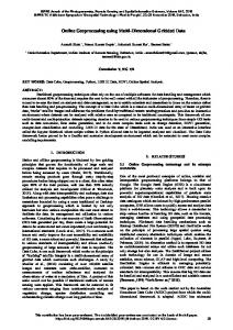
Given the individual images we first derive SIFT features (Lowe, 2004). Then, for each image pair (i, j) we compute the relative orientation parameters based on the 5-point algorithm of Nistér (2004) with RANSAC, record all inliers and compute the intersection angle for each matched feature pair (𝒑𝒊 , 𝒑𝒋 ). We choose the median of these angles as the intersection angle for the considered image pair. We keep all image pairs that fulfil two conditions: (a) they need to have more matches than a threshold (we use 50 in our work), and (b) at least a certain amount of the matches must be inliers (we use 80%). Among the remaining pairs, the one with an intersection angle closest to 90 degrees is the final choice for the initial image pair. The most obvious way to select the image to be added to the block next is to find the candidate which shares the most correspondences with the images employed so far. As it is not very efficient if only one image is added each time, we simultaneously add all images which fulfil two conditions (a) a certain percentage (we use 60%) of the features extracted from the image have matches to already computed 3D points, (b) the number of these features is above a threshold (we use 30 here). All images fulfilling these two conditions together with the images processed already are called a cluster. Then, rotation averaging (section 3.2), translation estimation (section 3.3) and resection refinement (Section 3.4) are performed independently for each new image of the cluster, followed by a local bundle adjustment (section 3.5) using the whole cluster. In the next step, from the remaining images a new cluster is formed and the procedure starts again. The procedure is visualised in Fig. 2.

be the rotation matrix of the new image that we want to estimate, 𝑹𝒊 , 𝑹𝒋 , 𝑹𝒌 , 𝑹𝒎 , 𝑹𝒏 are the rotation matrices previously estimated by iterative SfM for images i, j, k, m, and n, 𝑹𝒊𝒂 , 𝑹𝒋𝒂 , 𝑹𝒌𝒂 , 𝑹𝒎𝒂 , 𝑹𝒏𝒂 are the relative rotations with respect to image a calculated by the 5-point algorithm. We propagate the given rotations along these relative rotations to obtain different solu𝒋 𝒏 tions for 𝑹𝒂 , namely, 𝑹𝒊𝒂 , 𝑹𝒂 , 𝑹𝒌𝒂 , 𝑹𝒎 𝒂 , 𝑹𝒂 . We want to average these rotation matrices and obtain a robust result. Note that every rotation in SO(3) can be represented as a rotation by an angle α around an axis represented by unit 3-vector ̃𝐯 , v = α𝐯̃ subject to ‖𝐯̃ ‖2 =1; I is the identity matrix (see Hartley et al., 2013 for more details). Also, rotation matrices form a differentiable manifold which is inherent in every Lie group. According to Hartley et al. (2013), we project the rotation matrices to their Euclidean tangent space (the Lie algebra so(3)) using the logarithm log(·): SO(3)→ so(3): 𝐰

log(R) = [v]×, v = arcsin(‖𝐰‖2) ‖𝐰‖ , w = 2

𝐑−𝐑𝐓 𝟐

(1)

and 0 [v]× = ( 𝑣3 −𝑣2

−𝑣3 𝑣2 0 −𝑣1) 𝑣1 0

(2)

The inverse transformation projects so(3) back into SO(3) using the exponential map: R = exp([𝐯̃]×) = I +sin(α) [𝐯̃]×+(1-cos(α)) [𝐯̃]×2

(3)

We now want to estimate our rotation matrix R (matrix 𝑹𝒂 with reference to Fig. 3) from the different observations Ri (matrices 𝒋 𝒏 𝑹𝒊𝒂 , 𝑹𝒂 , 𝑹𝒌𝒂 , 𝑹𝒎 𝒂 , 𝑹𝒂 with reference to Fig. 3 ) by averaging the observations in tangent space: n

R = arg min ∑d( R , R i ) R

(4)

i =1

where d(R, 𝑹𝒊 ) = d(R, 𝑹𝒊 )geod = ||log(R𝑹𝑻𝒊 )||1 (geodesic distance).

Figure 2. Flowchart of our incremental image orientation method (for the explanation of “Ours” and “Ours_RF” see section 4.1). 3.2 Rotation estimation by single rotation averaging Given the rotation matrices of images, which have already been added to the block, and the relative rotations between those images and a newly added image, we can calculate several rotation matrices for the new image. With reference to Fig. 3 let 𝑹𝒂

Figure 3. Single rotation averaging (see text for more information). We use the L1 norm as it is more robust than the L2 norm, and apply the Weiszfeld algorithm to obtain the solution of (4). The pseudocode for single rotation averaging is presented in Algorithm 1, where 1/∑ni=1(1 ∕ ‖xi‖) determines the speed of convergence.


297


ν=Ax - b

Algorithm 1 Single rotation averaging Input a number of observations 𝑹𝒊𝒂 , i=1,2,3…n. ̅ Output mean rotation 𝑹 1. Initialize a rotation matrix 𝑹𝟎𝒂 by randomly choosing a rotation from all observations, 𝑹𝟎𝒕 = 𝑹𝟎𝒂 . Iteration number t = 0. 2. Do { For i =(1,2,3,…n) { 𝑻 xi = log(𝑹𝒊𝒂 ·𝑹𝟎𝒕 ); } δ = ∑ni=1(xi ∕ ‖xi‖)/∑ni=1(1 ∕ ‖xi‖); 𝑹𝟎𝒕+𝟏 = exp(δ) ·𝑹𝟎𝒕 ; t = t+1; } while (d( 𝑹𝟎𝒕+𝟏 , 𝑹𝟎𝒕 ) ≥0.0001or t 0.001, the observation of 𝑹𝒊𝒂 is discarded, such as the dotted line between 𝑹𝒂 and 𝑹𝒏𝒂 in Fig. 3. 4. Steps 2 and 3 are repeated until no observation can ̅ = 𝑹𝟎𝒕+𝟏 . be discarded and step 2 converges, 𝑹

argmin Ax - b x

3.4 Refinement of rotation and translation by space resection For each new image, the rotation estimated by Section 3.2 and translation estimated by Section 3.3 are regarded as an initial input for a space resection refinement to compute a more accurate result: M

minimize Ri ,Ti

r21 r22 r23

x ij - φ( K i , Ri ,Ti , X j )

j =1

(9) 2

3.5 Local bundle adjustment After having added all images selected according to section 3.1, and before adding a new cluster, we perform a bundle adjustment to reduce block deformation: N

minimize

r (X - X 0 ) + r21 ( Y - Y0 ) + r31 ( Z - Z0 ) x = -f 11 + x0 r13 (X - X 0 ) + r23 (Y - Y0 ) + r33 ( Z - Z0 )

r11 with 𝑹𝒊 = (r12 r13

∑

where i is the ID of the new image, M is the number of reconstructed scene points which can be viewed in the ith image, 𝑿𝒋 denotes its 3D point coordinates. 𝑹𝒊 , 𝑻𝒊 are the parameters that we aim to optimize. 𝑲𝒊 contains the intrinsic parameters (focal length and principal point), 𝝋 represents the collinearity equations (5), 𝒙𝒊𝒋 are the 2D image coordinates extracted from the ith image. These 2D and 3D points are assumed to be inliers as determined by sections 3.2 and 3.3.

Based on the rotation now known, image translation parameters can be estimated for the new image with only two 3D points: Using the collinearity equations, each 3D point yields two equations (5) and each image has three translation parameters ( X 0 , Y0, Z0 ). Thus, two 3D points with given image coordinates give four equations, which is enough to determine the three unknowns.

r12 (X - X 0 ) + r22 (Y - Y0 ) + r32 ( Z - Z0 ) + y0 r13 (X - X 0 ) + r23 ( Y - Y0 ) + r33 ( Z - Z0 )

(8)

1

Here, x and b are vectors constructed by concatenating the unknown translation parameters and the right part of equation (6), respectively; A is the coefficient matrix and ν is the vector of residuals. Equation (8) is based on the L1 norm. Normally, there are abundant 3D points that can be chosen to solve (6). We use RANSAC to find the best image translation.

3.3 Linear translation estimation for each new image

y = -f

(7)

Ri ,Ti , X j

(5)

r31 r32 ) r33

where (X, Y, Z) are the 3D coordinates of the jth object point 𝑿𝒋 which is assumed to be viewed by ith image, and (x, y) are the corresponding 2D image coordinates 𝒙𝒊𝒋 . ( x0 , y0 ) are the principal point coordinates of ith image, f is the focal length,. ( X 0 , Y0, Z0 ) are the coordinates of the unknown projection centre 𝑻𝒊 (equivalent to the image translation vector), and 𝑟𝑚𝑛 (m =1, 2, 3; n =1, 2, 3) are the entries of the rotation matrix 𝑹𝒊 . Note that for the simplicity, we omit the indices i and j in equation (5). To obtain a form which is linear in ( X0 , Y0 , Z0 ), we multiply equation (5) by the denominator: [( x - x 0 )r13 + fr11]X 0 + [( x - x 0 )r23 + fr21]Y0 + [( x - x 0 )r33 + fr31]Z0 = [( x - x 0 )r13 + fr11]X + [( x - x 0 )r23 + fr21]Y + [( x - x 0 )r33 + fr31]Z

M

∑∑ a

ij

x ij - φ( K i , Ri ,Ti , X j )

i =1 j =1

(10) 2

where N is the number of images and M is the number of scene points, 𝒂𝒊𝒋 = 1 if object point j can be viewed by image i, otherwise, 𝒂𝒊𝒋 = 0. 𝑹𝒊 , 𝑻𝒊 and 𝑿𝒋 are the items that we want to refine. 𝑲𝒊 again contains the intrinsic parameters. 𝝋 represents the collinearity equations (5), 𝒙𝒊𝒋 are the 2D image coordinates.

4. EXPERIMENTS In this section we present a detailed evaluation of our approach. We conduct experiment on three benchmark datasets (Strecha et al., 2008) consisting of 11 to 30 images and two datasets which have 128 ordered and 553 unordered images, respectively. Results of single rotation averaging are analysed by comparison with other methods (Section 4.1). We evaluate our translation estimation approach based on the ground truth of the three benchmark datasets (Section 4.2). To further demonstrate the potential of our approach, we orient the images of two larger datasets (Section 4.3). We use the open source Ceres-solver (Agawal et al., 2017) for bundle adjustment. 4.1 Evaluation of rotation results

[( y - y0 )r13 + fr12 ]X 0 + [( y - y0 )r23 + fr22 ]Y0 + [( y - y0 )r33 + fr32 ]Z0 = [( y - y0 )r13 + fr12 ]X + [( y - y0 )r23 + fr22 ]Y + [( y - y0 )r33 + fr32 ]Z

(6) Finally, we obtain the linear equation system (7) and the optimisation problem (8):

For the investigation of rotation accuracy, the three benchmark datasets fountain-P11, Herz-Jesu-P25 and castle-P30, which have known ground truth exterior orientation, are investigated. The interior orientation parameters are taken from the EXIF


298


information provided with the data. Fig. 4 shows results for different methods, the abscissa denotes the image ID, the ordinate is the angle error (in degrees), i.e. the difference between the computed value and ground truth (see appendix for computation). “Ours” is the result by just using the single rotation averaging (section 3.2). Applying resection refinement (see section 3.4) yields the results of “Ours_RF”. Note that while for all clusters but the last one, bundle adjustment has also been run as part of the procedure (see Fig. 2), the results used for “Ours” are those obtained directly after rotation averaging for all images. The same holds for the other experiments accordingly. “Res_RF” uses the DLT (Hartley & Zisserman, 2003) and is refined by resection refinement (see again section 3.4). “BA” denotes the results after final bundle adjustment. The initial image pairs of these datasets are (4,9), (4,9) and (4, 12), determined by the method described in Section 3.1, so the rotation of the fourth image is selected as the original one. The relative rotation between the fourth image and the corresponding ground truth is used to project all remaining rotation matrices into the coordinate system of the reference. We calculate the error  by comparing the ground truth rotations to the computed ones (see appendix for details). In this way, the error of the fourth image is always zero.

(a) fountain-P11

Comparing the angle errors of the different methods shown in Fig. 4, “Ours” provided by our single rotation averaging performs worst, probably due to remaining errors and outliers in the relative rotations. It can also be seen that the angle error of some images (for example image 10 in Fig.4(a) and images 10-13 and 20-25 in Fig.4(b)) are much larger than others. This is probably due to error accumulation. Errors propagate and accumulate when adding images of the new cluster sequentially into a refined block, and we found that the images which were added last have the largest angle errors. However, if we turn on the resection refinement, these results are significantly improved. Furthermore, by applying resection refinement, both “Ours_RF” and “Res_RF” achieve almost the same accuracy. As is expected, the angle errors after final bundle adjustment are the smallest ones: the errors for fountain-P11 and caslte-P30 are smaller than 0.4°, for Herz-Jesu-P25 smaller than 0.2°. In Tab. 1 we list the mean angle error of the mentioned methods along with the results of the baseline methods of Chatterjee and Govindu (2013) (“Global”), Jiang et al. (2015) and Reich and Heipke (2016). One can see that resection refinement has a strong effect on the accuracy of estimating rotations. Iit makes “Ours_RF” obtain the best results on fountain-P11 and caslteP30 (except for final bundle adjustment), while it also gives a similar accuracy as Reich and Heipke (2016) on Herz-Jesu-P25. Nevertheless, after final bundle adjustment, the results are significantly better. When comparing the different error norms, “Ours” (L1 norm) performs almost the same as “Ours_L2” (L2 norm, computed for comparison) on fountain-P11, but, on the other two datasets the L1 norm is much better; similar effects can be seen for “Global” and “G_L2”.

fountain-P11 Herz-Jesu-P25 castle-P30

Ours 0.316 0.785 1.236

Ours_L2 0.332 0.928 1.574

(b) Herz-Jesu-P25

(c) Castle-P30 Figure 4. Angle errors of three benchmark datasets. 4.2 Evaluation of translation result For the three benchmark datasets, a comparison of the translation accuracy is given in Fig. 5. Again, the abscissa denotes the image ID, the ordinate is the translation error (in decimetres). “Ours” means the method of our incremental linear translation estimation described in Section 3.3 based on rotations computed according to section 3.2, “Ours_RF” utilizes the resection refinement, “Res_RF” and “BA” denote as the same method as in Fig. 4. The translation error of castle-P30 and Herz-Jesu-P25 is two orders of magnitude larger than that of fountain-P11 (see ordinate in Fig. 5). Inspecting the results in more detail, we found that castleP30 and Herz-Jesu-P25 have lots of repetitive structures

before bundle adjustment Res_RF Global 0.18 0.251 0.152 0.27 0.231 0.238 0.443 0.745 0.338

Ours_RF

G_L2 0.261 0.365 0.954

(1) 0.249 0.206 0.583

(2) 0.45 0.39 0.96

after bundle adjustment Ours_RF 0.147 0.049 0.119

Table 1. Mean angle error in degree [ ͦ ] for different methods. We compared our results with Chatterjee and Govindu (2013) (Global), Reich and Heipke (2016) (1) and Jiang et al. (2015) (2). Res_RF denotes the “Res_RF” in Fig. 4. Ours_L2 uses the L2 norm to solve equation (4), G_L2 adopts the “Global” method with L2 norm. Note that we cite the results of (1) and (2) from the corresponding papers, and we reprogrammed the idea of Chatterjee and Govindu (2013) using the L1 and L2 norms.


299


and a significant number of image pairs with small intersection angles. Moreover, some images of castle-P30 are weakly connected; the block geometry of castle-P30 is not as dense as that of fountain-P11, which explains the findings. Similar to the angle error shown in Fig. 4, “Ours” always provides the worst results. This is probably a consequence of the results of rotation averaging (see section 4.1). Comparing Fig. 4 and Fig. 5, the images with large angle errors are normally solved with large translation errors, because these errors result in an inaccurate coefficient matrix A. “Ours_RF” and “Res_RF” give very similar results, which are much better than “Ours”. The performance after the final bundle adjustment is always the best; the translation errors of fountain-P11 are lower than 0.4 decimetres, both Herz-Jesu-P25 and castle-P30 have translation errors which are smaller than 2 decimetres.

Tab. 2 presents numerical results for the mean translation errors of different methods. Before final bundle adjustment, “Ours_RF” outperforms all other methods listed in Tab. 2. This means that optimization by resection refinement can improve the accuracy of translation and is a very important step in our pipeline. “Ours” detects and eliminates outliers of tie points iteratively, especially for those outliers from repetitive structures which pass the epipolar geometry verification. “Ours” is much better than the methods of Reich and Heipke (2016) and Jiang et al. (2015) on castle-P30. When comparing the error norms again, “Ours” (L1 norm) performs almost the same as “Ours_L2” on fountain-P11, but on the other two datasets the L1 norm works better. This is because Herz-Jesu-P25 and castle-P30 have more repetitive structures, so that some incorrect correspondences from these repetitive structures can survive epipolar geometry verification; wrong tie points corresponding to these correspondences will generate large residuals in equation (7). After final bundle adjustment, the results of “Ours_RF” are improved by one order of magnitude. Visualizations of image orientation results can be seen in Fig. 6.

(a) fountain-P11

(a) fountain-P11

(b) Herz-Jesu-P25

(c) castle-P30 Figure 6. Visualization of the orientation results on benchmark datasets after final bundle adjustment. (b)Herz-Jesu-P25

4.3 Experiment on other datasets

(c) castle-P30 Figure 5. Translation errors of three benchmark datasets

fountain-P11 Herz-Jesu-P25 castle-P30

Ours 0.387 1.66 2.87

Ours_L2 0.362 1.83 2.96

To further demonstrate the performance of our approach, we used two additional datasets. Building from Zach et al. (2010) has 128 ordered images. Notre Dame provided by Wilson and Snavely (2014) has 553 unordered images. To detect mutual overlap these unordered images for efficient image matching, Zhan et al. (2015, 2018) propose two methods based on visual vocabulary trees and random k-d trees respectively. However, these two methods were only proven to be work well on a small set of images. The approach of Wang et al. (2017) is applied in this paper. The ground truth of building is not available. We used the incremental system contained in the OpenMVG library (Moulon et al., 2016) to do orientation, and the result is regarded as ground truth. The translation error of building has [pixels] as units.

before bundle adjustment Ours_RF Res_RF 0.271 0.23 1.224 0.81 1.37 1.27

(1) 0.35 0.83 13.12

(2) 0.72 0.61 16.20

after bundle adjustment Ours_RF 0.08 0.16 0.16

Table 2. Mean translation error in decimetre for different methods. Ours_L2 uses L2 norm to solve equation (7).


300


Wilson and Snavely (2014) provided the ground truth for Notre Dame. In Tab. 3 we present a comparison of the “Ours_RF” results with the ground truth. For the rotations the results are in the same range as those of the benchmark datasets; the translation results seem to be reasonable, too. After final bundle adjustment (BA), rotations and translations are again improved. Visualizations of the image blocks after BA are shown in Fig. 7. Ours_RF

Before BA

After BA

R [ ]ͦ 0.49 T [pixel] 1.86 Notre Dame R [ ]ͦ 0.52 T [m] 2.06 Table. 3 Mean rotation error and translation error and Notre Dame by Ours_RF. building

0.18 0.94 0.26 1.66 of building

𝛼 = trace(𝑹𝒊 𝑹−𝟏 𝒋 ) /3

(11)

Where 𝑹𝒊 𝑹−𝟏 𝒋 is the difference matrix between 𝑹𝒊 and 𝑹𝒋 and 𝛼 is the average value of the main diagonal elements of 𝑹𝒊 𝑹−𝟏 𝒋 . We can compute the angular error 𝜃 by 𝜃 = arccos(𝛼) ∙ 180/ 𝝅

(12)

ACKNOWLEDGEMENTS The author Xin Wang would like to thank the China Scholarship Council (CSC) for financially supporting his PhD study at Leibniz Universität Hannover, Germany.

REFERENCES Abdel-Aziz, Y.I.; Karara H.M., 1971. Direct linear transformation from comparator coordinates into object-space coordinates. ASP Symp. Close-Range Photogrammetry, University of Illinois, Urbana, Ill., USA, pp. 1-18. Agarwal, S., Mierle, K. et al., 2007. Ceres Solver. http://ceressolver.org (accessed 08.05.2017). . (a) building

Agarwal, S., Snavely, N., Simon, I., Seitz, S. M., Szeliski, R., 2009. Building Rome in a day. In: Proceedings of the IEEE International Conference on Computer Vision (ICCV), pp.72-79. Arie-Nachimson, M., Kovalsky, S.Z., Kemelmacher-Shlizerman, I., Singer, A., Basri, R., 2012. Global motion estimation from point matches. In: Proceedings of the International Conference on 3D Imaging, Modeling, Processing, Visualization and Transmission (3DIMPVT), pp. 81–88. Arrigoni, F., Fusiello A., Rossi B., 2016. Camera motion from group synchronization. In: Proceedings of the IEEE International conference on 3D Vision (3DV), pp.546-555.

(b) Notre Dame Figure 7. Visualization of orientation results on the building and Notre Dame datasets after final bundle adjustment.

5. CONCLUSIONS In this paper, we present a new robust incremental image orientation method by combining the information of relative rotations and tie points. First, rotations of newly added images are determined by single rotation averaging. Then, a linear translation estimation method is proposed to determine the translation parameters of these newly added images. The evaluation using three benchmark datasets demonstrates that our approach performs well. Moreover, experiments on the challenging building and Notre Dame datasets demonstrate that it is also possible to orient larger sets of both ordered and unordered images. Inspired by the incremental method, we next plan to build a large linear equation system to determine all translation parameters simultaneously. This makes sense if rotations are available from a global rotation averaging scheme.

APPENDIX: ROTATION ERRORS Given two similar rotations 𝑹𝒊 and 𝑹𝒋 , 𝜃 is the angle difference we want to compute. We start by computing a value 𝛼:

Chatterjee, A., Govindu, V.M., 2013. Efficient and robust largescale rotation averaging. In: Proceedings of the IEEE International Conference on Computer Vision (ICCV), pp. 521– 528. Cui, Z., Jiang, N., Tang, C., Tan, P., 2015. Linear global translation estimation with feature tracks. In: Proceedings of the British Machine Vision Conference (BMVC). Cui, H., Gao, X., Shen, S., Hu., Z., 2017. HSfM: Hybrid Structure-from-Motion. In: Proceedings of the IEEE Conference on Computer Vision and Pattern Recognition (CVPR), pp. 12121221. Farenzena, M., Fusiello, A., Gherardi, R., 2009. Structure-andmotion pipeline on a hierarchical cluster tree. In: Proceedings of the IEEE International Conference on Computer Vision (ICCV) Workshop, pp. 1489-1496. Govindu, V.M., 2001. Combining two-view constraints for motion estimation. In: Proceedings of the IEEE Conference on Computer Vision and Pattern Recognition (CVPR), 2, pp. II–218. Goldstein, T., Hand, P., Lee, C., et al., 2016. Shapefit and shapekick for robust, scalable structure from motion. In: Proceedings of the European Conference on Computer Vision (ECCV). Springer, pp.289-304.


301


Hartley, R., Zisserman, A., 2003. Multiple View Geometry in Computer Vision. Cambridge University Press. Hartley, R., Aftab, K., Trumpf, J., 2011. L1 rotation averaging using the Weiszfeld algorithm. In: Proceedings of the IEEE Conference on Computer Vision and Pattern Recognition (CVPR), vol. 1, pp. 3041–3048. Hartley, R., Trumpf, J., Dai, Y., Li, H., 2013. Rotation averaging. Int. J. Comp. Vis. (IJCV) 103 (3), 267–305. Havlena, M., Torii, A., Knopp, J., Pajdla, T., 2009. Randomized Structure from Motion Base on Atomic 3D Models from Camera Triplets. In: Proceedings of the IEEE Conference on Computer Vision and Pattern Recognition (CVPR), pp.2874-2881. Jiang, N., Cui, Z., Tan, P., 2013. A global linear method for camera pose registration. In: Proceedings of the IEEE International Conference on Computer Vision (ICCV), pp. 481– 488. Jiang, N., Lin,W.-Y., Do, M. N., Lu, J., 2015. Direct structure estimation for 3d reconstruction. In: Proc. IEEE Conference on Computer Vision and Pattern Recognition (CVPR), pp. 2655– 2663. Lowe, D.G., 2004. Distinctive Image Features from Scale-invariant Keypoints. International Journal of Computer Vision, 60(2), pp. 91–110. Martinec, D., Pajdla, T., 2007. Robust rotation and translation estimation in multiview reconstruction. In: Proceedings of the IEEE Conference on Computer Vision and Pattern Recognition (CVPR), pp. 1–8. Mayer, H., 2014. Efficient hierarchical triplet merging for camera pose estimation. In: German Conference on Pattern Recognition– GCPR 2014. Springer, Berlin, pp. 99–409. Moulon, P., Monasse, P., 2012. Unordered feature tracking made fast and easy. European Conference on Visual Media Production, CVMP. Moulon, P., Monasse, P., Marlet, R., 2013. Global fusion of relative motions for robust, accurate and scalable structure from motion. In: Proceedings of the IEEE International Conference on Computer Vision (ICCV). Moulon, P., Monasse, P. and others, 2016. OpenMVG: An Open Multiple View Geometry library. https://github.com/openMVG/openMVG (accessed 23.07.2017). Nistér, D., 2004. An efficient solution to the five-point relative pose problem. IEEE Trans. Pattern Anal. Mach. Intell. 26 (6), pp.756–770.

Reich, M., Yang, M. Y., Heipke, C., 2017. Global robust image rotation from combined weighted averaging. ISPRS Journal of Photogrammetry & Remote Sensing, 127, pp.89-101. Schönberger, J. L., Frahm, J. M., 2016. Structure-from-Motion Revisited. In: Proceedings of the IEEE Conference on Computer Vision and Pattern Recognition (CVPR). Snavely, N., Seitz, S. M., Szeliski, R., 2006. Photo tourism: exploring photo collections in 3d. Acm Transactions on Graphics, 25(3), pp.835-846. Strecha, C., von Hansen, W., Van Gool, L., Fua, P., Thoennessen, U., 2008. On benchmarking camera calibration and multi-view stereo for high resolution imagery. In: Proceedings of the IEEE Conference on Computer Vision and Pattern Recognition (CVPR), pp. 1–8 Toldo, R., Gherardi, R., Farenzena, M., Fusiello, A., 2015. Hierarchical structure-and-motion recovery from uncalibrated images. Computer Vision & Image Understanding, 140, pp.127143. Wilson, K., Snavely, N., 2014. Robust global translations with 1DSFM. In: Proceedings of the European Conference on Computer Vision (ECCV). Springer, pp. 61–75 Wu, C. 2013. Towards Linear-Time Incremental Structure from Motion. In: Proceedings of the IEEE Conference on 3dtv, pp.127134. Wang, X., Zhan, Z. Q., Heipke, C., 2017. An efficient method to detect mutual overlap of a large set of unordered images for structure-from. ISPRS Ann. Photogramm. Remote Sens. Spatial Inf. Sci., IV-1-W1, pp.191-198. Zach, C., Klopschitz, M., Pollefeys, M., 2010. Disambiguating visual relations using loop constraints. In: Proceedings of the IEEE Conference on Computer Vision and Pattern Recognition (CVPR), pp. 1426–1433. Zheng, Y., Kuang, Y., Sugimoto, S., Okutomi, M., 2013. Revisiting the PnP Problem: A Fast, General and Optimal Solution. In: Proceedings of the IEEE International Conference on Computer Vision (ICCV), pp.2344-2351. Zhan, Z. Q., Wang, X., Wei, M. L., 2015. Fast method of constructing image correlations to build a free network based on image multivocabulary trees. Journal of Electronic Imaging, 24(3):033029. Zhan, Z. Q., et al., 2018. Optimization of incremental structure from motion combining a random kd forest and pHash for unordered images in a complex scene. Journal of Electronic Imaging, 27(1):013024.

Ozyesil, O., Singer, A., 2015. Robust camera location estimation by convex programming. In: Proceedings of the IEEE Conference on Computer Vision and Pattern Recognition (CVPR), pp. 2674-2683. Reich, M., Heipke, C., 2015. Global rotation estimation using weighted iterative lie algebraic averaging. ISPRS Ann. Photogram., Rem. Sens. Spatial Inf. Sci. 1, pp.443–449. Reich, M., Heipke, C., 2016. Convex image orientation from relative orientations. ISPRS Annals of Photogrammetry Remote Sensing & Spatial Informa, III-3, pp.107-114.


302

robust image orientation based on relative rotations ... - ISPRS Annals

robust image orientation based on relative rotations ... - ISPRS Annals

Suggest Documents

convex image orientation from relative orientations - ISPRS Annals

robust and accurate image-based georeferencing ... - ISPRS Annals

robust and accurate image-based georeferencing ... - ISPRS Annals

sensor simulation based hyperspectral image ... - ISPRS Annals

relative pose estimation from airborne image sequences - ISPRS Annals

subpixel mapping of hyperspectral image based on ... - ISPRS Annals

robust feature tracking in image sequences using view ... - ISPRS Annals

rectification and robust matching using oriented image ... - ISPRS Annals

skyline matching based camera orientation from ... - ISPRS Annals

AGENT BASED MODELING - ISPRS Annals

object-based image analysis of worldview-2 satellite ... - ISPRS Annals

Realtime Image Matching for Vision Based Car ... - ISPRS Annals

image-based topography reconstruction by minimizing ... - ISPRS Annals

evaluation of matching strategies for image-based ... - ISPRS Annals

image-based reconstruction and analysis of dynamic ... - ISPRS Annals

evaluation of matching strategies for image-based ... - ISPRS Annals

ISPRS Paper - ISPRS Annals

ISPRS Paper - ISPRS Annals

ISPRS Paper - ISPRS Annals

an improved unsupervised image segmentation ... - ISPRS Annals

research on image translation between sar and optical ... - ISPRS Annals

Robust extraction of image correspondences ... - ISPRS Archives

orientation and dense reconstruction of unordered ... - ISPRS Annals

sensor-topology based simplicial complex ... - ISPRS Annals