Feb 15, 2001 - believe that the pursuit of the engineering goal of building an autonomous outdoor tour guide for Rice University, a tree-filled oasis in the urban ...
Robust localization algorithms for an autonomous campus tour guide Richard Thrapp and Christian Westbrook and Devika Subramanian Department of Computer Science Rice University, Houston TX 77005, USA � richardt,cw,devika � @cs.rice.edu February 15, 2001 Abstract This paper describes a robust localization method for an outdoor robot that gives tours of the Rice University campus. The robot fuses odometry and GPS data using extended Kalman filtering. We propose and experimentally test a technique for handling two types of non-stationarity in GPS data quality: abrupt changes in GPS position readings caused by sudden obstructions to line of sight access to satellites, and more gradual changes caused by disparities in atmospheric conditions. We construct measurement error covariance matrices indexed by number of visible satellites and switch them into the localization computation automatically. The matrices are built by sampling GPS data repeatedly along the route and are updated continuously to handle drift in GPS data quality. We demonstrate that our approach performs better than extended Kalman filters that use only a single error covariance matrix. With a GPS receiver that delivers 1 meter accuracy, we have been able to localize good to 40 cm through a challenging route in the Engineering Quadrangle of Rice University.
1 Introduction Our goal is to build an autonomous mobile robot that gives tours of the Rice University campus (see Figure 2). While there are many successful mobile robots that autonomously navigate and explore indoor environments like museums [13, 10] and offices [8] over extended periods of time, there are far fewer examples1 in the outdoor arena, most being research prototypes [1, 3, 11, 12, 6]. There are several reasons why the design of autonomous outdoor robots is challenging: outdoor environments vary more than those indoors, and we do not have good characterizations for them, and robust solutions to the localization �
We thank the George R. Brown School of Engineering, Rice University for its generous support of our work. 1 The new grass mowing robots guided by externally placed wires at lawn boundaries and around obstacles are not considered here, because they require the environment to be instrumented for them.
problem for outdoor robots are still under development. We believe that the pursuit of the engineering goal of building an autonomous outdoor tour guide for Rice University, a tree-filled oasis in the urban metropolis of Houston, will help us make progress on the scientific goal of characterizing outdoor environments for which reliable mobile robot navigation algorithms can be designed and built. This paper describes the localization algorithms used by our robot, their integration with the navigation algorithms, and presents preliminary experimental results. An important ground rule we followed to ensure portability of our methods was to allow no instrumentation or modification of our environment. A key issue for outdoor robots is the choice of sensors for performing localization. While indoor robot localization algorithms make extensive use of sonars [14, 13, 5], they are virtually useless for outdoor robots, as the environment consists mostly of vast open spaces where the sensors return no valid range information. They are, however, useful (together with bump sensors) for local obstacle avoidance. With a view to determining the smallest set of sensors needed to provide robust localization and navigation in a campus environment, we have currently limited ourselves to data from odometry, which provides location and orientation information relative to a start position, and GPS, which provides global positioning and heading data. Our objective is to understand experimental limits on the accuracy of localization achievable using just these two sources of information. 2 Our robot needs to give tours throughout the day without requiring human intervention. It therefore requires localization accuracies of at least 40 cm at all times during its entire operation. This is about half the width of the walkways around our campus. Unlike office environments in which short term localization errors are generally nonfatal, small errors can have catastrophic consequences for our outdoor robot e.g., falling off of a curb or missing a sidewalk and rolling onto a busy street. 2 We plan to add vision to our robot to augment odometry and GPS for localization.
It is well known that dead-reckoning using pure odometry is not a very robust localization technique for robots [2, 6] that cover long distances, and are in continuous operation over extended periods of time. This is because errors in odometry accumulate over time due to inaccuracies in the kinematic model, precision limitations of encoders, and unobservable factors like wheel slippages that are not accounted for in the kinematic equations. Kalman filtering of carefully calibrated odometric data with state measurement signals provided by a redundant sensor (e.g., a gyroscope) can provide significant improvements [6]. However, they still cannot on their own provide localization accuracies of 40 cm over extended periods of time, as needed for our problem. GPS is now a standard technique for obtaining absolute position information for outdoor robots [6, 3, 11, 1, 12]. Our GPS receiver (an Invicta 210S) can provide position information accurate to about a meter ( ����� �� � �� ). It also provides estimations of the current heading by using the Doppler shift of the satellite signals. The accuracy of this estimate depends greatly on the speed at which the GPS antenna is moving, but at the top speed of our robot, we have determined that ��������� � � radians. Differential GPS systems like RTK GPS can provide centimeter level resolution, however they cost an order of magnitude more, and their performance is very sensitive to the number of visible satellites [3]. GPS information alone is not sufficient to achieve the localization accuracies needed for our application, because the tour guide’s route on our campus is largely covered with trees and runs very close to tall buildings which obstruct line of sight access to the GPS satellites. Further, atmospheric conditions degrade the quality of the GPS signals in varying ways at different locations. In this paper, we adapt Extended Kalman Filtering (EKF) [7, 9] used in [6, 3, 12] for mobile robot localization to fuse odometry and GPS data. Our innovation is the addition of a dynamic mechanism to handle non-stationarities in GPS data quality. Because of the rapid change in quality of GPS data when the view of satellites is obstructed in an urban campus environment, the standard approach of using a single covariance matrix to model measurement errors in GPS data is not adequate. This approach necessitates artificially increasing variances more than is usually needed, causing slower convergence of the Kalman filter. If the data quality diminishes suddenly, the Kalman filter does not account for the reduction in quality quickly enough, and our robot performs poorly because inaccurate GPS data is weighted too heavily. Conversely, if our robot gains a line-of-sight path to additional satellites after having adapted to a reduced quality GPS signal, the increased variances cause the Kalman filter to not take advantage of the higher quality data, so control errors in our robot accrue again. We show that by using a finite number of error
covariance matrices in different GPS quality situations, creating them as needed and updating them dynamically, it is possible to handle changes in GPS signal quality quickly and effectively. The paper is organized as follows: In Section 2, we give a brief description of the tour guide task as well the mechanical and sensor configuration of our robot. We lay out the basic EKF algorithm upon which our localization algorithm is based. We then describe the extension to the EKF algorithm that dynamically constructs error covariance matrices to handle non-stationarities in the GPS data quality. Section 3 contains a brief discussion of issues in designing control algorithms for navigation that use position and heading estimates produced by the localization algorithm. In Section 4, we provide details of our experiments and demonstrate that the dynamic measurement error covariance matrix generation handles rapid changes in GPS signal quality well. We conclude with a brief summary of our ongoing work in designing methods for human interaction with our robot.
2 The Tour Guide Task and Robot 2.1 The task and the robot The tour guide task requires the ability to navigate in a dynamic, uninstrumented, potentially dangerous (vehicular traffic on streets, sharp curbs, moving obstacles such as animals and people, etc.) urban environment. In addition, the robot needs to interact with a tour group in an interesting and informative manner. Interaction is tightly interwoven with navigation: the robot needs to be aware of its location so it can use its location context to answer questions appropriately. Our tour guide robot is an ATRV Jr. from RWI Inc, named Virgil3 (Figure 1). It is a four-wheeled robot designed for outdoor use and comes equipped with an array of sonars and odometry. We added a GPS receiver used typically in marine applications which receives real-time corrections from the Coast Guard station at Galveston. We also added touch-sensitive bumpers for obstacle detection and avoidance. The wheels on the same side of the robot are mechanically coupled. The raw encoder information is not directly available, neither do we have access to the full kinematic model of the robot which is used by the on-board odometry computation to provide integrated measures like distance traveled and change in orientation in a given sampling interval. Both odometric and GPS data are sampled at 10Hz in our robot. 3 Virgil
is named after the guide in Dante’s Inferno.
Movement Translational Rotational
Systematic Error -0.0290 -0.0492
Random Error 0.0036 0.0589
Table 1: Systematic errors and random error variances measured in odometry related to the two types of motion supported.
Figure 1: Virgil: The Rice campus tour guide
2.2 Odometry Before integrating data from different sources, we calibrated the odometry using the GPS receiver. Because odometry measures the number of rotations in the wheels rather than the actual distance traveled, several sources of error can accumulate. Largely, systematic error is due to tire size miscalculations: as the tires wear down, the amount of linear distance traversed reduces in comparison to the number of rotations the tires travel. In addition, because the tires are constantly being worn down, this analysis must be reperformed periodically to estimate new systematic error values. This error can be directly compensated for by scaling the commands given to the drive system. In addition, other sources of error such as slippage and surface imperfections result in a random component to the error whose variance can also be approximated through repeated trials. By traveling, according to odometry, in straight lines for fairly large distances (20 meters), and comparing the odometry’s results for distance traveled with GPS data averaged over 100 readings, we are able to determine approximate values for systematic and random errors in odometry. In addition, to limit the effect of systematic inaccuracies in translating GPS coordinates into local coordinates, we performed the test from many different starting positions and headings. It is possible that this method reports a slightly higher than actual random error rate due to GPS inaccuracies. To determine turning error, we follow a similar procedure of moving forward a distance and using GPS data at the endpoints of that movement to approximate the current heading, using odometry to turn a preset angle, and then move forward again to calculate the true angle turned using averaged GPS data. This is inherently less accurate than calculating distance over a straight path, but gives a reasonably good approximation of the true errors. Again, because of GPS inaccuracies, the random component in the measured error will likely be larger than the true random error. After performing these tests, we observed that our robot’s odometry consistently under-maneuvered both
while traveling in straight lines and while turning as a result of the smaller than expected size of the worn tires. These results are presented in Table 1 as a ratio of error to distance traveled for 29 trials of both the translational and rotational measurements which approximates the actual error. Systematic error is accounted for directly in the odometry system, increasing the robot’s perception of how far it has traveled by the appropriate ratio, and random error is handled as uncertainty in the data fusion process.
2.3 Extended Kalman Filter Kalman filtering is a well known technique for state and parameter estimation [7, 9]. The standard Kalman filter assumes that the controlled process is governed by a linear stochastic difference equation. An extended Kalman filter handles non-linear stochastic processes by linearizing about the current mean and covariance. In the 2D outdoor robot localization problem, the state of the robot is its position and orientation ����������� � in a fixed frame of reference. The state (0,0,0) is the geographic center of the Rice campus (Baker Fountain). All �!�"�#�$� positions are measured in centimeters north and east relative to this location, and the orientation � is the angle from due north. The robot’s state evolves according to the following system of non-linear stochastic difference equations. The state of the system at time % is ����&$�#��& ���'&'� . The wheel encoders yield, at each sampling period the translation (*)!& along the heading �'& and a rotation (,+�- . These equations relate the state at time %/.0� to the state at time % , and the internally sensed translation (*)!& in the direction �'& and rotation (�+#in the interval between times % and %1.�� . The zero mean vector 23&4�657�! 98;:/&?�
�*&3.@ BA'C��'&D(*)!&E.723&�F
��&�=�>G�
��&H.ICKJML,�'&�(*)!&E.723&�N
� &�=�>
� & .7( +�- .72 &K+
�
These equations can be summarized as follows, where C�& is the state of the system at time % and (,&O�P��(*)!& ��(,+�-T�
UV�WCD& ��(,& ��23& �
We use the GPS signal to determine the measurement error between the actual state and the internally computed state above. We model the measurement process as follows X &Y�
CD&3.7Z &
C &�=�>#_`&
�
&�=�>#_`&
�
UV�WC B& _`& ��(,& �# � a bc& &B_`& bd&'ef.@:/&
g
&�=�>#_`& stands for our prediction of the state vector for time %O.h� given internal sensor information from time % and a knowledge of the state at time % . &�=�>#_`& is the a priori
estimate of the error covariance, i.e. the covariance of the difference between the actual state and the state predicted on the basis of measurements till time % . bc& is the Jacobian of the process UV�i�j� with respect to the state vector g �k�!�"�����#��� . By differentiating the state evolution equation with respect to C , we obtain the following matrix: lm
o (p)!&