Robust Optimization-Based Scheduling of Multi-Microgrids ... - MDPI

energies Article

Robust Optimization-Based Scheduling of Multi-Microgrids Considering Uncertainties Akhtar Hussain, Van-Hai Bui and Hak-Man Kim * Department of Electrical Engineering, Incheon National University, 12-1 Songdo-dong, Yeonsu-gu, Incheon 406-840, Korea; [email protected] (A.H.); [email protected] (V.-H.B.) * Correspondence: [email protected]; Tel.: +82-32-835-8769; Fax: +82-32-835-0773 Academic Editor: João P. S. Catalão Received: 19 February 2016; Accepted: 1 April 2016; Published: 9 April 2016

Abstract: Scheduling of multi-microgrids (MMGs) is one of the important tasks in MMG operation and it faces new challenges as the integration of demand response (DR) programs and renewable generation (wind and solar) sources increases. In order to address these challenges, robust optimization (RO)-based scheduling has been proposed in this paper considering uncertainties in both renewable energy sources and forecasted electric loads. Initially, a cost minimization deterministic model has been formulated for the MMG system. Then, it has been transformed to a min-max robust counterpart and finally, a traceable robust counterpart has been formulated using linear duality theory and Karush–Kuhn–Tucker (KKT) optimality conditions. The developed model provides immunity against the worst-case realization within the provided uncertainty bounds. Budget of uncertainty has been used to develop a trade-off between the conservatism of solution and probability of unfeasible solution. The effect of uncertainty gaps on internal and external trading, operation cost, unit commitment of dispatchable generators, and state of charge (SOC) of battery energy storage systems (BESSs) have also been analyzed in both grid-connected and islanded modes. Simulations results have proved the robustness of proposed strategy. Keywords: forecasted load uncertainty; optimal operation; microgrid scheduling; multi- microgrids; renewable generation uncertainty; robust optimization

1. Introduction A typical microgrid (MG) comprises of various distributed generations (DGs), energy storage systems (ESSs), and loads and it can operate in both grid-connected and islanded modes [1]. Microgrids have the ability to sustain penetration of renewable generations (RGs), plug-in hybrid vehicles, and energy storage systems. In addition, MGs can support the main distribution system by supplying/absorbing power [1]. Microgrids also have an enormous potential to provide service reliability, reduce emissions, and improve power quality for the end-use customers through the utilization of DGs, ESSs, and DR programs. In order to achieve the fore-mentioned benefits of MGs, penetration of renewable generation resources and DR programs has significantly increased in the recent years. This enhanced penetration has imposed new challenges to the scheduling of microgrids [2]. Various forecasting techniques are used for forecasting the electric load demands [3], demand response (DR) [4], and RGs [5] (wind and solar generations) considering various environmental factors like wind speed [6], solar irradiance [7], and weather intelligence and history data [8]. However, due to various unpredictable natural phenomena, these forecasted values are not accurate. Owing to the significance of uncertainties associated with power generation of RGs and forecasted load demands in microgrids, uncertainty management has become an active research area in scheduling of MG systems in the recent years. Conventionally spinning and non-spinning reserves have been used for managing the uncertainties associated with the distribution Energies 2016, 9, 278; doi:10.3390/en9040278

www.mdpi.com/journal/energies

Energies 2016, 9, 278

2 of 21

systems [9]. However, in the past few years, various novel techniques have been introduced by researchers for managing the uncertainties in microgrids. Sensitivity analysis [10], fuzzy logic-based optimization [11], stochastic optimization techniques [12], and robust optimization [13–16] are among the noticeable techniques available in the literature for uncertainty management in scheduling of active distribution systems and microgrids. The drawbacks associated with each of the uncertainty management technique are summarized in the following paragraphs. The discrepancy between the forecasted values and realization has been relatively small in the conventional distribution systems [9]. Therefore, reserves have been commonly used for catering these minor discrepancies. However, in multi-microgrid systems this solution is not feasible. Sensitivity analysis being a post-operation analysis technique is not capable of providing any immunity against the uncertainties. Determination of membership functions in a fuzzy programming is based on personal experience of decision makers and is somewhat free and subjective [17]. Due to the limitations of these techniques, stochastic and robust optimization techniques have been widely used for uncertainty management of microgrids. The prominent disadvantages associated with the stochastic optimization-based uncertainty management of microgrids are increase in problem size and computational requirements with increase in number of scenarios, dependence of accuracy on scenario generating technique [14], provision of probabilistic guarantee for feasibility of solution [2], and requirement of accurate information of uncertainty for generation of precise probability distribution functions (PDFs) [13]. In contrast to stochastic optimization, RO only requires moderate information of underlying uncertainties (uncertainty bounds) [2], provides immunity against all possible realizations of uncertain data within the uncertainty bounds, and formulation of tractable models even for large systems [9]. These features of RO along with many other related appealing features have attracted the attention of researchers in the recent years. In addition to scheduling of microgrids [13–16], RO has also been used for optimization of various other related objectives of power systems which includes, distributed generation investments [18], transmission network expansion [19], DG placement [20], transition of electric vehicles (EVs) [21], scalability of DR [22], communication in microgrids [23], and many more. Architecture of energy management system (EMS) plays a vital role in the scheduling of MGs/MMGs. Therefore, various EMS strategies have been investigated by the research community. A centralized EMS strategy has been proposed by [24] for scheduling of microgrids while, an optimal energy management for cooperative multi-microgrid community has been proposed by [25,26]. Distributed energy management strategies have been used for scheduling of microgrids by [27,28]. Both the centralized and distributed strategies have their own merits and demerits, which are highlighted by [26,29]. Hybrid and hierarchical optimization schemes have also been used for scheduling of microgrids in the recent years [26,29]. Due to the merits of cooperative MMG communities highlighted by [25,26], a cooperative MMG community has been used for testing the feasibility of the proposed optimization strategy. Most of the researches available in the literature on RO-based scheduling [1,2,9,13–17] of MGs are concentrated on a single microgrid. However, in order to fully benefit from MGs, networking of various MGs to form a multi-microgrid (MMG) system has emerged in the literature as an advanced form and application of single MGs [30]. This interconnection may result in escalation of uncertainties, especially if the MGs lie within the same metrological locality (which is commonly practiced). A feasible solution for the worst-case realization of the MMG system is more challenging and desirable than single MGs. Even for single MGs, RO has been primarily used for uncertainty management of renewable energy sources only [2,9,14,15,17]. However, load uncertainty has become equally challenging and equally important problem for microgrids. In this paper, RO has been used for scheduling of multi-microgrid systems considering uncertainty in both output of renewable energy sources and forecasted load values. Initially, a deterministic model has been formulated for the MMG system. Then, it has been transformed to a non-linear robust counterpart and finally, a tractable robust counterpart has been formulated. The objective of the

Energies Energies 2016, 2016, 9, 9, 278 278

33 of of 21 21

objective of the developed model is to minimize the daily operation cost of the MMG system in developed model is to under minimize daily operation bounds. cost of the MMG system in grid-connected grid-connected mode the the given uncertainty Due to the higher penalty cost ofmode load under the given uncertainty bounds. Due to the higher penalty cost of load shedding in islanded shedding in islanded mode, service reliability becomes more essential than operation cost. The mode, service more thancost operation cost.commitment The results of proposed results of the reliability proposed becomes algorithm likeessential operation and unit of the controllable algorithm like operation cost and unit commitment of controllable generators, and BESSs remain valid generators, and BESSs remain valid even if the loads and/or renewable power outputs fluctuate even if the loads and/or renewable power outputs fluctuate (within the provided uncertainty bounds). (within the provided uncertainty bounds). Therefore, the robustness of the proposed approach can Therefore, robustness the proposed approach can besolutions defined as its ability to operate and provide be defined the as its ability toofoperate and provide feasible under the bounded uncertainties. feasible solutions under the bounded uncertainties. The conservatism of the solution and probability The conservatism of the solution and probability of unfeasible solution under the given uncertainty of unfeasible under the givena uncertainty bounds can be byInselecting suitable bounds can besolution controlled by selecting suitable value of budget of controlled uncertainty. order toaquantify value of budget of uncertainty. In order togaps quantify impact of uncertainties, gaps have the impact of uncertainties, uncertainty havethe been determined for eachuncertainty case (uncertainty in been determined for each case (uncertainty in renewable power sources, uncertainty in electric loads, renewable power sources, uncertainty in electric loads, and uncertainty in both renewable energy and uncertainty in both renewable energy sources loads). The developed have sources and electric loads). The developed models and haveelectric been simulated using CPLEX models in Microsoft been simulated using CPLEX in Microsoft visual studio environment. visual studio environment. 2. Uncertainty UncertaintyManagement ManagementininMicrogrids Microgrids 2. Microgrid operation operation based based on on deterministic deterministic optimization optimization as as shown shown in in Figure Figure 1a, 1a, neglects neglects the the Microgrid forecast errors. However, the uncertainties of load and renewable energy are important issues for forecast errors. However, the uncertainties of load and renewable energy are important issues for economic and and secure secure operation operation of of microgrids microgrids [1]. [1]. Conventionally, Conventionally, uncertainties uncertainties in in power power systems systems economic have been handled by imposing conservative reserve requirements. It is easy to implement practice. have been handled by imposing conservative reserve requirements. It is easy to implement practice. However, itit could economically inefficient wayway to commit extraextra resources as reserve to handle However, couldbebeanan economically inefficient to commit resources as reserve to uncertainty [2]. Additionally, multi-microgrid systems may still face capacity shortfall when the handle uncertainty [2]. Additionally, multi-microgrid systems may still face capacity shortfall when real-time conditions deviates significantly from the the expected values. the real-time conditions deviates significantly from expected values. a

Forecasted Values

Realization

Electrical Energy

b

Scenarios Realization

c

Realization

Upper Bounds

Lower Bounds t

t+1

t+2 Time Intervals

t+3

t+4

Figure Figure 1. 1. Uncertainty Uncertainty representation: representation: (a) (a)Deterministic Deterministic optimization; optimization; (b) (b) Stochastic Stochastic optimization; optimization; and and (c) (c) Robust Robust optimization. optimization.

Sensitivity analysisisiscarried carried to assess the impact of forecasting on operations microgrid Sensitivity analysis outout to assess the impact of forecasting errors onerrors microgrid operations system [31]. it is analysis a post-optimal analysis is not and system and security [31].security However, it isHowever, a post-optimal technique and is technique not capableand of directly capable of directly identifying an optimal scheduling strategy in terms of minimizing the uncertainty identifying an optimal scheduling strategy in terms of minimizing the uncertainty for achieving for achieving aimmunity guaranteed immunity against any real-timeFuzzy-optimization discrepancy. Fuzzy-optimization has also a guaranteed against any real-time discrepancy. has also been emerged been emergedfor asdealing a candidate for dealing with uncertainties in scheduling of microgrids. as a candidate with uncertainties in scheduling of microgrids. In fuzzy-optimization, the In fuzzy-optimization, the errors in the forecast load, wind speed, and solar irradiance can be taken errors in the forecast load, wind speed, and solar irradiance can be taken into account through fuzzy into account through fuzzy clustering sets [32]. Fuzzy clustering used to account for seasonal sets [32]. Fuzzy logic-based is usedlogic-based to account for seasonalisvariations. These fuzzy sets are variations. These fuzzy sets are known as membership functions. known as membership functions.

Energies 2016, 9, 278

4 of 21

However, the selection of these fuzzy sets is specific to the experience of the decision makers and is somewhat free and subjective [17]. Stochastic optimization has been widely used for scheduling of uncertainty-aware microgrids. However, due to various limitations of stochastic optimization and numerous advantages of robust optimization, RO has gained tremendous popularity in optimization of microgrids. Figure 1b shows a stochastic optimization approach and Figure 1c shows the RO approach. It can be observed that RO only needs information about the upper and lower bounds of uncertainty. The major Energies drawbacks associated with the stochastic optimization and merits of RO can be summarized 2016, 9, 278 4 of 21 as follows. ‚

‚

‚

‚

However, the selection of these fuzzy sets is specific to the experience of the decision makers and is somewhat free and subjective [17]. Stochastic optimization has been widely used for Stochastic optimization only provides probabilistic guarantee to the feasibility of solution while, scheduling of uncertainty-aware microgrids. However, due to various limitations of stochastic RO provides immunity against advantages all possibleofrealizations of the uncertain data within a deterministic optimization and numerous robust optimization, RO has gained tremendous popularity optimization of microgrids. Figure 1b shows a stochastic optimization approach and uncertainty setin[2]. Figure 1c shows the RO approach. It can be observed that RO only needs information about the In stochastic optimization large number of scenarios are required to ensure quality of the upper and lower bounds of uncertainty. The major drawbacks associated with the stochastic scheduling solution which results growth of optimization and merits of RO can bein summarized as problem follows. size and computational requirements,

while RO puts the random problem parameters in a deterministic uncertainty set including the  Stochastic optimization only provides probabilistic guarantee to the feasibility of solution worst-case scenario and the robust against modelallremains tractable forwithin all cases [15]. while, RO provides immunity possible computationally realizations of the uncertain data a deterministic uncertainty set [2]. In case of stochastic optimization, accurate information of uncertainties is required to construct  In stochastic largeuncertainties number of scenarios are i.e., required to and ensure quality of the and need accurate PDFs, whileoptimization RO describes by sets, upper lower bounds scheduling solution which results in growth of problem size and computational requirements, not assume probability distributions [18]. while RO puts the random problem parameters in a deterministic uncertainty set including the The accuracy of solution is sensitive the remains technique used for scenario generation in stochastic worst-case scenario and the robustto model computationally tractable for all cases [15].  In case of stochastic accurate information uncertainties is required to construct optimization but RO onlyoptimization, needs information about theofupper and lower bounds [18]. accurate PDFs, while RO describes uncertainties by sets, i.e. upper and lower bounds and need

not assume probability distributions In 1970, Soyster adopted linear robust [18]. optimization for the first time. Due to conservativeness  The accuracy of solution is sensitive to the technique used for scenario generation in stochastic under worst-case constraints, this technique has not gained much popularity [18]. These conservative optimization but RO only needs information about the upper and lower bounds [18]. property problems have been resolved by [33], by proposing the concept of adjustable robust 1970, Soyster adopted linear robust optimization for the first time. Due to conservativeness optimization. InHowever, the complexity of robust counterpart was still an issue. The complexity under worst-case constraints, this technique has not gained much popularity [18]. These issue has conservative been resolved by introducing an resolved adjustable parameter bythe [34,35]. parameter has property problems have been by [33], by proposing concept That of adjustable been named as budget of uncertainty is decided by the decisionwas makers. can robust optimization. However, theand complexity of robust counterpart still anThis issue.parameter The complexitybetween issue hasthe been resolved of byrobustness introducing and an adjustable parameter by [34,35]. ensure a trade-off objective economy. This method has That been used for parameter has been named as budget of uncertainty and is decided by the decision makers. This optimization of multi-microgrids in this paper. parameter can ensure a trade-off between the objective of robustness and economy. This method The breakdown stepsofin a robust optimization-based processing of uncertain data is has been used of for major optimization multi-microgrids in this paper. shown in Figure Estimation of upper lower uncertainty bounds be donedata using The 2. breakdown of major steps in and a robust optimization-based processingcan of uncertain is historic shown in Figure 2. Estimation of upper and lower bounds can be done using historic data [36] or confidence intervals [37]. A review onuncertainty neural network-based prediction intervals has data [36] or confidence intervals [37]. A review on neural network-based prediction intervals has been carried out by [38] for determining confidence intervals. After determining the upper and lower been carried out by [38] for determining confidence intervals. After determining the upper and bounds, a lower deterministic model is formulated. bounds, a deterministic model is formulated. Formulate MILP Deterministic Model

Formulate Worst-Case Model

Historic Data

Confidence Interval

Estimate Upper and Lower Bounds

Identify SubProblem

Decide Degree of Conservatism

Find Dual of Sub-Problem

Calculate Budget of Uncertanity

Formulate Trackable Robust Counterpart

Formulate MILP Robust Counterpart

Figure 2. Problem formulation process of robust optimization.

Figure 2. Problem formulation process of robust optimization.

Energies 2016, 9, 278

5 of 21

The deterministic model is then transformed into the worst-case model. The worst-case Energies 2016, 9, 278 5 of 21 model contains a sub-problem; linear duality theory is applied to the sub-problem. By applying The deterministic model is then transformed worst-case model. The worst-case model by Karush-Kuhn-Tucker (KKT) optimality conditionsinto andthe decided value of budget of uncertainty contains a sub-problem; linearcounterpart duality theory is formulated. applied to the By applying decision makers, a traceable robust can be Thesub-problem. budget of uncertainty is used Karush-Kuhn-Tucker (KKT) optimality conditionsand andthe decided value of of uncertainty to formulate a trade-off between the conservatism probability of budget unfeasible solutions by within decision makers, a traceable robust counterpart can be formulated. The budget of uncertainty is the given uncertainty bounds. The relationship between the error probability of unfeasible solution used to formulate a trade-off between the conservatism and the probability of unfeasible solutions and budget of uncertainty for independent and symmetrically distributed random variables in r´1, 1s within the given uncertainty bounds. The relationship between the error probability of unfeasible has been formulated by [35]. solution and budget of uncertainty for independent and symmetrically distributed random variables in [−1, 1] has been formulated by [35].

3. System Model

3. System Modelnetwork of three heterogeneous microgrids (MG , MG , and MG ) has been A cooperative 1 2 3 considered this study. The basic components of each microgrid renewable sources A in cooperative network of three heterogeneous microgrids (MG1are , MG 2, and MGenergy 3) has been considered in this study. The basic components of each microgrid are(CS) renewable sources (photovoltaic (PV) array, wind turbine (WT), and concentrated solar power energy unit), controllable (photovoltaic (PV)(CG), array,battery wind turbine andsystem concentrated power unit), controllable distributed generator energy(WT), storage (BESS),solar and(CS) electric load. Each MG contains distributed generator (CG), battery energy storage system (BESS), and electric load. Each MG type at-least one of the three renewable energy sources. CGs in all microgrids are assumed to of same contains at-least one of the three renewable energy sources. CGs in all microgrids are assumed to of with different generation capacities. BESS capacity has also been assumed to be different for each MG. same type with different generation capacities. BESS capacity has also been assumed to be different All the MGs are inter-connected and connected to the utility grid, such that they can trade energy for each MG. All the MGs are inter-connected and connected to the utility grid, such that they can with the utility grid and with other MGs of the network. Proposed MMG system can also operate in trade energy with the utility grid and with other MGs of the network. Proposed MMG system can islanded illustration of An theillustration MMG system shown in Figure 3. in Figure 3. also mode. operateAn in islanded mode. of theisMMG system is shown Each Each MG sends its information to thetocommunity EMS EMS (CEMS). This information includes capacity MG sends its information the community (CEMS). This information includes and state of charge (SOC)ofofcharge BESS, (SOC) forecasted values of renewable generators with generators uncertaintywith bounds, capacity and state of BESS, forecasted values of renewable uncertainty values ofbounds, load withand uncertainty and capacity and per-unit forecasted valuesbounds, of loadforecasted with uncertainty capacity bounds, and per-unit generation cost of each generation cost of each the CG units. CEMS receives market price signals (buying and selling prices)grid. CG units. CEMS receives market price signalsthe(buying and selling prices) from the utility from the utility grid. After receiving all the component-related information from each MG andfrom After receiving all the component-related information from each MG and market price signals market price signals from the utility grid, CEMS performs optimization of the MMG system with an the utility grid, CEMS performs optimization of the MMG system with an objective to minimize the objective to minimize the operation cost of the MMG system under worst-case realization. CEMS is operation cost of the MMG system under worst-case realization. CEMS is responsible for scheduling responsible for scheduling the resources of each MG. Each MG has to follow the scheduling the resources of each MG. Each MG has to follow the scheduling commands received from the CEMS. commands received from the CEMS.

Figure 3. An illustration of a typical multi-microgrid system.

Figure 3. An illustration of a typical multi-microgrid system.

Energies 2016, 9, 278

6 of 21

4. Problem Formulation Optimal operation of MGs is considered as the uppermost level of microgrid control. The control levels in MGs are due to difference in significance and time scale for each control level [39]. Each lower level of control is a prerequisite for the upper level control. Therefore, constraints related to the lower levels’ control are assumed to be satisfied in each of the upper level control. The proposed approach is meant for economic scheduling of MMGs, therefore, lower level controls like internal voltage and current control of DRs, voltage and frequency deviations compensation, and load flow analysis, have not been included (assumed to be fulfilled). A robust optimization formulation is developed to deal with the uncertainties of renewable power sources and forecasted load demands. The developed robust model is based on mixed integer linear programming (MILP) and the robustness of the model can be adjusted against the level of conservatism of the solution. The proposed model is formulated for a 24-h scheduling horizon with a time interval of t, which could be any uniform interval of time. However, in the proposed scheduling t has been assumed to be one hour. 4.1. Deterministic Model 4.1.1. Objective Function The objective of the deterministic model is to minimize the following objective function. The objective function comprises the operating costs, start-up and shut-down costs of CGs, total cost of buying electricity from the utility grid, total profit gained by selling electricity to the utility grid in grid-connected mode, and penalty cost for shedding load in islanded mode respectively. um ptq P t0, 1u is operation mode indicator of MMG system. um ptq = 1 implies that the mth MG is connected to the main grid and 0 indicates the islanded mode. min

T ř M ř G ´ ř t“1 m“1 g“1

´ ¯ ¯ CG pCG ptq ` SUC CG ptq ` SDC CG ptq PUCm,g m,g m,g m,g `

`

T ř M ` ř t“1 m“1 T ř M ř t“1 m“1

˘ BUY ptq ´ C SELL ptq .pSELL ptq .u ptq C BUY ptq .pm m m

(1)

SHED .pSHED ptq . p1 ´ u ptqq Cm m m

4.1.2. Load Balancing Constraints For each MG, the total amount of power generated from the local sources and BESS charging/discharging power must be kept equal to the local load demand and power exchanged with the utility grid and other MGs of the network in grid-connected mode. However, in islanded mode, load shedding might be used for balancing the load as represented by Equation (2a). LOAD ptq ´ pSHED ptq . p 1 ´ u ptqq ` pCHR ptq ` st ptq .pSE ptq “ p GEN ptq ` p GRID ptq pm m m m m m m m DCR ptq ` r f ptq .p RE ptq ; @m, t `pm m m GRID ptq “ pm GEN pm ptq “

G ÿ

´

¯ BUY ptq ´ tgm ptq .pSELL ptq f gm ptq .pm . um ptq ; @m, g, t m

WT PV CS pCG m,g ptq ` wtm .pm ptq ` pvm .pm ptq ` csm .pm ptq ; @m, t

(2a) (2b) (2c)

g “1

pvm ptq , wtm ptq , csm ptq , f gm ptq , tgm ptq , r f m ptq , stm ptq , um ptq t0, 1u ; @m, t

(2d)

LOAD ptq ď pm ptq ; @m, t r f m ptq ` stm ptq “ 1; f gm ptq ` tgm ptq “ 1; pSHED m

(2e)

Equation (2a) is the power balancing equation. While, Equation (2b) shows the trading power with the utility grid and Equation (2c) gives the total local generations (controllable and renewable).

Energies 2016, 9, 278

7 of 21

Equation (2d) shows the binary variables associated with the renewable generations (pvm , wtm ,csm ), power trading with the utility grid ( f gm , tgm ), and power trading among microgrids (r f m , stm ), respectively. Equation (2e) depicts the fact that simultaneous buying/selling from/to the utility grid, and simultaneous sending/receiving to/from other MGs is not possible for a given MG at time t. 4.1.3. Constraints for Controllable Generators Equation (3a)–(3e) show the imposed constraints for distributed controllable generators. In Equation (3a), sm,g ptq is a binary variable and it shows the commitment status of CG g in MG m at time interval t. If CG is committed to operate in time t, this binary variable takes the value of 1and 0otherwise. Power generation limits of gth CG in mth MG are given by Equation (3a). Equation (3b) shows the relationship between the start-up indicator (sum,g ptq) and shut-down indicator (sdm,g ptq). If the gth CG is started up at time t, start-up indicator will take the value of 1 and zero otherwise. Similarly, the shutdown indicator will take a value of 1, if the gth CG is shut-down at time t and zero otherwise [30]. Equation (3c) and (3d) show the constraints related to start-up and shut-down costs, respectively. Equation (3e) portrays the fact that at any given time t, any CG cannot be started up and shut down simultaneously. ” ı ” ı CG CG min Pm,g .sm,g ptq ď pCG m,g ptq ď max Pm,g . sm,g ptq ; sm,g ptq P t0, 1u ; @m, g, t

(3a)

sum,g ptq ´ sdm,g ptq “ sm,g ptq ´ sm,g pt ´ 1q ; @m, g, t ` ˘ CG CG CG SUCm,g ptq ě UCm,g ptq . sm,g ptq ´ sm,g pt ´ 1q ; SUCm,g ptq ě 0; @m, g, t ` ˘ CG CG CG SDCm,g ptq ě DCm,g ptq . sm,g pt ´ 1q ´ sm,g ptq ; SDCm,g ptq ě 0; @m, g, t

(3b)

(3d)

sum,g ptq ` sdm,g ptq ď 1; sum,g ptq , sdm,g ptq P t0, 1u ; @m, g, t

(3e)

(3c)

4.1.4. Energy Trading Constraints The power exchange between the mth MG and utility grid is limited by the capacity of the corresponding line connecting them. Equation (4a) shows this limitation for trading power with the utility grid. The binary variables as defined in Equation (2e) allow the mth MG to either buy or sell GRID ptq will be positive if the power from/to the utility grid at a given time interval t. The value of pm MG buys powers from the utility grid and will be negative if the MG sells power to the utility grid at any time interval t [30]. GRID ptq ď PmCAP ; @m, t ´ PmCAP ď pm (4a) CAP 0 ď ppSE m,nq ptq ď stm ptq .Ppm,nq ; @m, n, t; @m ‰ n

(4b)

CAP 0 ď ppRE m,nq ptq ď r f m ptq .Ppm,nq ; @m, n, t; @m ‰ n

(4c)

DEF 0 ď ppRE ptq ; @m, n, t; @m ‰ n m,nq ptq ď pm

(4d)

SUR ptq ; @m, n, t; @m ‰ n 0 ď ppSE m,nq ptq ď pm

(4e)

M ÿ N ÿ m “1 n “1

ppRE m,nq ptq “

N ÿ M ÿ

ppRE n,mq ptq ; @m, n, t; @m ‰ n

(4f)

n “1 m “1

The power exchange between any two connected MGs (m and n) is limited by the capacity of the corresponding line connecting them. Equation (4b) and (4c) show these limitations for sending power from mth MG to nth MG and receiving power by mth MG from nth MG, respectively. The value ptq will be positive, if MG m sends power to MG n and it will be zero otherwise. Similarly, the of ppSE m,nq value of ppRE ptq will be positive if MG m receives power from MG n and vice versa. Equation (2e) m,nq allows each MG to either send or receive power at time interval t. Equation (4d) constraints each MG

Energies 2016, 9, 278

8 of 21

for receiving only deficit amount of power from other microgrids, i.e., prohibits selling of received power and (4e) restricts each MG for sending only surplus power to other MGs of the network, i.e., prohibits from buying while sending power. Finally, Equation (4f) shows that amount of power sent and received to/from MGs of network should be balanced at each time interval t. 4.1.5. Battery Constraints

Energies 2016, 9, 278 

8 of 21 

mth

8 of 21  The limits and dynamics of electrical energy8 of 21  stored in 8 of 21  the BESS of MG are given by 4.1.5. Battery Constraints  Equation (5a) and (5b). Equation (5c) and (5d) show the charging and discharging limits of BESS, Constraints    respectively. Equation (5e) shows constraints related to initial of of  themsimulation frame th  MG  are time The  limits  and  dynamics  of  the electrical  energy  stored  in  the step BESS  given  by  I N IT as the initial SOC of the BESS. Equation (5f) depicts that BESS cannot be charged and with P th th th m in  Equation  (5a)  and  (5b).  Equation  (5c) and  and  discharging  limits  of  BESS,  namics  ts  electrical  and  dynamics  of  energy  electrical  of  stored  energy  electrical  stored  the  energy  BESS  in  the  of  stored  mBESS  in  of  the  mBESS  of  mshow    MG  are   given  MG (5d)  are  by  given    MG the  are  by charging  given  by  discharged simultaneously. The timeand  interval (time forof  BESS modeling will be in accordance to respectively. Equation (5e) shows the constraints related to initial step of the simulation time frame  Equation  5c) and  and  (5b).  (5d)  (5c) and  Equation  show  (5d)  the  (5c) and  charging  show (5d)  the and  charging  show  discharging  the and  charging  discharging  limits  of discharging  BESS,  limits  of step) BESS,  limits  BESS,  Energies 2016, 9, 278  8 of 21  8 of 21  defined time stepinitial  in problem formulation, one hour this study. with  as  the  SOC  of  the  BESS.  i.e., Equation  (5f) indepicts  that  BESS  cannot  be  charged  and  Equation (5e) shows the constraints related to initial step of the simulation time frame  he constraints related to initial step of the simulation time frame  e) shows the constraints related to initial step of the simulation time frame 

78 

” that  ıBESS  ” ı discharged simultaneously. The time interval (time step) for BESS modeling will be in accordance to  SOC  e  the  BESS.  initial  of  the  Equation  SOC  BESS.  of  (5f)  Equation  the depicts  BESS. (5f)  Equation  that  depicts  BESS  (5f)  that  cannot  depicts  BESS  be  cannot  charged  be and  cannot  charged be  and  charged  and  nts  4.1.5. Battery Constraints  BESS SOC BESS Energies 2016, 9, 278  8 of 21  8 of 21  min P ď p ptq ď max P ; @m, t (5a) m m m defined time step in problem formulation, i.e. one hour in this study.  me interval (time step) for BESS modeling will be in accordance to  multaneously. The time interval (time step) for BESS modeling will be in accordance to  sly. The time interval (time step) for BESS modeling will be in accordance to  th th dynamics  The  of limits  electrical  and energy  dynamics  stored  of  electrical  in  the  BESS  energy  of  mstored  the  BESS    MG in  are  given  by of  m   MG  are  given  by  blem formulation, i.e. one hour in this study.  ulation, i.e. one hour in this study.  tep in problem formulation, i.e. one hour in this study.  Energies 2016, 9, 278  8 of 21  8 of 21  4.1.5. Battery Constraints  aints  (5a)  max ;p DCR ∀ , ptq   mindischarging  ).  Equation  Equation (5c) and  (5a)  and (5d)  (5b).  show  Equation  the  charging  (5c) and  and  (5d)  show  the  charging  limits  of  and  BESS,  discharging  limits  of  BESS,  m SOC SOC CHR CHR p ptq “ p pt ´ 1q ` p ptq .η ´ ; @m, t (5b) m m (5a)  max max ; ∀of stored  , electrical    max ;min  ∀ the  , energy    BESS  ;m∀stored  ,  mth(5a)  min limits  DCR th  (5a)  d  dynamics  The  of  min electrical  and  dynamics  energy  of  the  BESS  of  m  in  MG  are  given  by  MG  are  given  by   (5e) shows the constraints related to initial step of the simulation time frame  respectively. Equation (5e) shows the constraints related to initial step of the simulation time frame  Energies 2016, 9, 278  8 of 21  8 of 21  ηm aints  4.1.5. Battery Constraints  (5b)  1 . ; ∀ ,   ¸ limits  ˜cannot  “depicts  ‰ and  Equation  5b).  Equation  and  (5c) and  (5b).  (5d)  Equation  show  (5c) and  the  (5d)  show  and  discharging  the  charging  limits  of  discharging  BESS,  of  BESS,  with  al  SOC  of (5a)  the as  BESS.  the  initial  Equation  SOC  (5f)  of  depicts  the charging  BESS.  that  Equation  BESS  (5f)  be  charged  that  BESS  and  cannot  be  charged  and  1 limits  1 . dynamics  1 . of  .   CHR ; ∀ ,in  ; ∀BESS  ,   stored  ;m∀th(5b)  ,mBESS   the  ptby  ´th1q max ´(5b)  pSOC  aints  dynamics  The  of  electrical  and  energy  stored  electrical  the  energy  of  in  BESS  m  P MG  are  given   (5b)  MG  are  given  by  m of  4.1.5. Battery Constraints  respectively. Equation (5e) shows the constraints related to initial step of the simulation time frame  on (5e) shows the constraints related to initial step of the simulation time frame  ously. The time interval (time step) for BESS modeling will be in accordance to  discharged simultaneously. The time interval (time step) for BESS modeling will be in accordance to  (5c) .cm ptq ; @m, t 0 ď pm ptq ď CHRof  0(5d) and  . ; limits  ∀ ,  of  BESS,  (5c)  5b).  Equation  Equation  (5a)  (5c) and  and  (5b).  (5d)  Equation  show  the  (5c) and  charging  show  discharging  the  charging  limits  discharging  BESS,  ηcharged  mand  with  itial  SOC  of  as  the  the  BESS.  initial  Equation  SOC  of  the  (5f)  BESS.  depicts  Equation  that  BESS  (5f)  cannot  depicts  be  that  BESS  cannot  and  be  charged  and  roblem formulation, i.e. one hour in this study.  defined time step in problem formulation, i.e. one hour in this study.  th th d  The  limits  and  dynamics  energy  of  the are  BESS   in  given  by    (5c)  MG  are  given  by  0dynamics  0of  electrical  . ; stored  ∀electrical  . ,   in ; the  ∀energy  .,BESS    stored  ; of  ∀ m, (5c)    MG  (5c)  ” of  m ´´ ı¯¯ on (5e) shows the constraints related to initial step of the simulation time frame  respectively. Equation (5e) shows the constraints related to initial step of the simulation time frame  neously. The time interval (time step) for BESS modeling will be in accordance to  discharged simultaneously. The time interval (time step) for BESS modeling will be in accordance to  SOC BESS DCR(5d)  and  DCR 0 1 min . ; ∀BESS,  , (5a)    t . charged  (5d)  Equation  5b).  Equation  (5a)  and  (5c) and  (5b).  (5d)  Equation  show  (5c) and  the  charging  show  discharging  the  charging  limits  and  of  discharging  BESS,  limits  pt ´ 1qbe  ´that  min ptq .ηm .dm of  ptq ; @m, (5d) p(5f)  0 ďBESS.  pm ; Equation  max ∀ ,ď  BESS  max ; ∀ BESS  ,P(5a)    and  min min with  tial  SOC  of  as  the  the  BESS.  initial  Equation  SOC  of  the  (5f)  depicts  that  depicts  charged  cannot  be  and  m cannot  m defined time step in problem formulation, i.e. one hour in this study.   problem formulation, i.e. one hour in this study.  0 1 min 1 min . 1 min . ; ∀ ,   . ; ∀ ,   ; ∀ ,   . . . respectively. Equation (5e) shows the constraints related to initial step of the simulation time frame  on (5e) shows the constraints related to initial step of the simulation time frame  (5d)  (5d)  (5d)  1 1;  ∀ ,   (5e)  eously. The time interval (time step) for BESS modeling will be in accordance to  discharged simultaneously. The time interval (time step) for BESS modeling will be in accordance to  SOC I N IT ´ “be  Pthat  i f(5b)  “ 1;, @m, t charged (5a)  (5e) (5b)  with  itial  SOC  of  as the  the BESS.  initial  SOC  of  depicts  Equation  depicts  BESS  cannot  and  be  and  1 Equation  . (5f)  1that  . 1q ; ,∀pBESS  ,   ptcannot  ;t ∀   (5e)  m (5f)  mcharged  (5a)  max ; ∀   max ; ∀ ,   1 min 1 1;  ∀1min ,  the  1; BESS.  ∀ ,   1;  ∀ , (5e)  (5e)  problem formulation, i.e. one hour in this study.  defined time step in problem formulation, i.e. one hour in this study.  1;    ∊ 0,1 ; 0   +    ,  , 1; ∀ , (5f)  neously. The time interval (time step) for BESS modeling will be in accordance to  discharged simultaneously. The time interval (time step) for BESS modeling will be in accordance to  CHR DCR ptq P t0, dm c,m ptq, , d(5f)  ; 0 ď ηm , ηm ď 1; @m, t (5f) m1; ∀ ; defined time step in problem formulation, i.e. one hour in this study.  1;  1;  1; 0   ∊   , 0,1 ∊ ` 0,1 0 , “ 1;1; ∀    , +  , ;c0m.  ptq 1; ∀ , ; ptq , 1u (5a)  (5a)  min   ∊  , 0,1 (5b)  (5b)   problem formulation, i.e. one hour in this study.  .,   ,,    (5f)  0 0minmax . 1 ; ; ∀ ∀ , , ; ∀   max .; ∀ , ;(5f)  ;   ∀∀(5c)  (5c)  4.2. Robust Counterpart  4.2. Robust Counterpart (5a)  (5a)  min min max (5b)  (5b)  . ,  ; ∀ ,   01 1 0 min ..1 ; ∀ ;,max ∀ .,  ,   . ; ∀ . ;  ,∀  ;. ∀ . 1;  ,∀;   ∀min (5d)  (5d)  unterpart  0 ,   (5c)  The  next step step  robust  optimization‐based  problem  is  to (5c)  formulate  a  robust  The next in in  robust optimization-based problem solvingsolving  is to formulate a robust counterpart 1 1 1;  ∀ , formulate   1 is solving  1;  ∀formulate  ,robust   ; ∀(5e)  (5e)  of  the  robust  (5b)  (5b)  . 1 . ; ∀ ,   ,   counterpart  of  the  deterministic  model  as  depicted  by  Figure  2.  The  purpose  ptimization‐based  t robust  step 0 in  optimization‐based  robust  problem  optimization‐based  solving  problem  is  solving  problem  to  to  formulate  a  robust  is  to  a  a  robust  of0 the deterministic model of the robust . . 1 as; .depicted ∀min,   ; ∀ by, Figure ; . 2.∀ The ,  (5c)  (5c)  counterpart is to 1 0 min  . . ; ∀purpose ,   (5d)  (5d)  erministic  model  f +  the  deterministic  as model  depicted  as  by  depicted  as  depicted  2.  Figure  by  2.  The of  purpose  2.  The  robust  the  robust  the  robust  1;  counterpart is to overcome the drawbacks introduced by uncertainties [40]. The uncertainty bounds  ∊ by  0,1 ;The  1;  0 purpose    the  ∊by0,1 0purpose    , model   Figure  +   the  ,, Figure  1; ∀ , ;of  , of  1; ∀ , overcome drawbacks introduced uncertainties [40]. The uncertainty bounds (5f)  (5f)  are formulated 1 1 0 min 1; .1∀. 1,   ; . ∀min,  ; ∀ 1;  ∀. ,   ; . ∀ ,  (5d)  (5e)  (5e)  are formulated prior to worst‐case model realization, in order to cater the influence of intermittent  me the drawbacks introduced by uncertainties [40]. The uncertainty bounds  wbacks introduced by uncertainties [40]. The uncertainty bounds   to overcome the drawbacks introduced by uncertainties [40]. The uncertainty bounds  0 . (5c)  (5c)  0 ,   ; ∀ ,   (5d)  prior to worst-case model realization, in order to cater the influence of intermittent renewable power renewable power generation and variable customer loads.  d prior to worst‐case model realization, in order to cater the influence of intermittent  worst‐case model realization, in order to cater the influence of intermittent  model realization, in order to cater the influence of intermittent  1;    ∊ variable 1;  0,1 ; 0 0,11; ∀ ;0 ∀   +    +  ,   ∀1,  ,   ,   ∊loads. , , 1; ∀ , (5f)  (5f)  generation and 1;  customer (5e)  (5e)    4.2. Robust Counterpart  0 1 1 min . 1 . min ; ∀ 1;  ,   . ,  . ;∀ ,   (5d)  (5d)  wer generation and variable customer loads.  ariable customer loads.  tion and variable customer loads.  1;  4.2.1. Uncertainty Bounds    ∊problem  0,1 1; Bounds ; 01; solving    ∊ to  0,1 ;0    , +   ∀,  ,  , is  1; ∀ , , solving  1; ∀ , (5f)  (5f)  n   +  robust  The  optimization‐based  next  step  in  robust  optimization‐based  problem  formulate  is  to  formulate  a (5e)  robust  4.2.1. Uncertainty 1 1;  ∀   , a  robust  (5e)  art  4.2. Robust Counterpart 1 eterministic  counterpart  model  of  the  as  deterministic  depicted  by  Figure  model  2.  as  The  depicted  purpose  by  Figure  of  the  2.  robust  The  purpose  of  the  robust  s  nty Bounds  is assumed  assumed that the variables should be made  made before(5f)  the revealing  revealing of  of the  the It  be  before  the  1;    ∊ 1;  0,1that  ; 0  all   decision ∊ 0,11; ∀ ; 0variables    +    It +  , is  , all the  , decision  , , should  1; ∀ , (5f)   4.2. Robust Counterpart  in  The  robust  next  optimization‐based  step  in  robust  optimization‐based  problem  solving  is  problem  to  formulate  solving a is  robust  to  formulate  a  robust  come the drawbacks introduced by uncertainties [40]. The uncertainty bounds  counterpart is to overcome the drawbacks introduced by uncertainties [40]. The uncertainty bounds  art  uncertainty from the  the renewable energy sources and electricof loads.  loads. The bounded  bounded variables  variables for  for uncertainty  from  renewable  energy  sources  electric  umed  ecision  all  the  that  variables  decision  all  the  should  variables  decision  be should  variables  made  before  be should  made  the before  be  revealing  made  the before  revealing  of  the the and  of  revealing  the  the  The  counterpart  deterministic  of model  the  deterministic  as  depicted  model  by  Figure  as  depicted  2.  The  by  purpose  Figure  of 2. the  The  robust  purpose  of  the  robust  o worst‐case model realization, in order to cater the influence of intermittent  are formulated prior to worst‐case model realization, in order to cater the influence of intermittent  LOAD PVfor  WT ptq, CS ptq) ˆ ˆ ˆ ˆ electric load ( p ptq) and renewables power generations ( p ptq, p p are given by electric  load  ( ̂ )  and  renewables  power  generations  ( ̂ ,  ̂ ,  ̂ )  are  given  by  energy  newable  om  the  sources  renewable  energy  and  sources  energy  electric  and  sources  loads.  electric  The  and  loads.  bounded  electric  The  loads.  variables  bounded  The  variables  bounded  variables  for  for   counterpart is to overcome the drawbacks introduced by uncertainties [40]. The uncertainty bounds  in renewable power generation and variable customer loads.  robust  The  next  optimization‐based  step  in  robust  moptimization‐based  problem  solving  is problem  to  formulate  solving  a  is  robust  to  formulate  m m a  robust  m art  4.2. Robust Counterpart  ercome the drawbacks introduced by uncertainties [40]. The uncertainty bounds  eration and variable customer loads.  LOAD ) and renewable  Equation (6a)–(6d). The symmetrical uncertainties associated with load (∆ ptq) Equation symmetrical associated withby  load ( pmrobust  and renewable ̂ renewables  wables  and  power  )  and  generations  renewables  power  generations  ((6a)–(6d). power  ̂ ,  generations  ̂ (The ̂ Figure  , as  , ̂ depicted  ̂ (2. ̂ ) The  are  ,  , uncertainties ̂ given  ̂ ) Figure  are  by  ,  of  ̂ given  ) The  by  are  given  counterpart  deterministic  of  model  the  deterministic  as  depicted  model  by  purpose  by  2.  the  robust  purpose  of  the  are formulated prior to worst‐case model realization, in order to cater the influence of intermittent  r to worst‐case model realization, in order to cater the influence of intermittent  PV solving  WT CS   in  The  robust  next  optimization‐based  step  in  robust  optimization‐based  problem  is  problem  to  formulate  solving  a  is  robust  to  formulate  a  robust  power  generations  (∆ , ∆ , ∆ )  lie  within  the  upper  and  lower  bounds  given  by  ) and renewable  ) and renewable  ) and renewable  –(6d). The symmetrical uncertainties associated with load (∆ symmetrical uncertainties associated with load (∆ al uncertainties associated with load (∆ power generations ( p ptq , p ptq , p ptq) lie within the upper and lower bounds given ercome the drawbacks introduced by uncertainties [40]. The uncertainty bounds  counterpart is to overcome the drawbacks introduced by uncertainties [40]. The uncertainty bounds  m m m nds  4.2.1. Uncertainty Bounds  eneration and variable customer loads.  renewable power generation and variable customer loads.  LOAD PV WTof  the CSrobust  counterpart  deterministic  of  model  the  deterministic  as  depicted  model  by  Figure  as  depicted  2.  The  by  purpose  Figure  of  2.  the  The  robust  purpose  tions  (∆ , ∆ , ∆ )  lie  , ∆ , ∆ within  )  lie  , the  ∆ within  upper  )  lie  the  and  within  upper  lower  the  and  bounds  upper  lower  given  and  bounds  lower  by  given  bounds  by  given  by  ptq ptq ptq ptq) by Equation (6a)–(6d). The upper bounds (p , p , p , p and lower bounds Equation  (6a)–(6d).  The  upper  bounds  ( m , m , r to worst‐case model realization, in order to cater the influence of intermittent  are formulated prior to worst‐case model realization, in order to cater the influence of intermittent  m , m )  and  lower  bounds  PV CS ptq) should  ercome the drawbacks introduced by uncertainties [40]. The uncertainty bounds  counterpart is to overcome the drawbacks introduced by uncertainties [40]. The uncertainty bounds  at  all  the  It  is  decision  assumed  variables  that  the  decision  be  made  variables  the  revealing  be  made  of quantities before  the  bounds  the (load revealing  of  the  generators) ptq ptq ptq (p,LOAD ,all  p(should  pWT , , ) for the uncertain quantities (load and renewable generators) can be  pbefore  for the uncertain and renewable )–(6d).  e  bounds  upper  The  ( bounds  upper  ( bounds  , , , , , )  and  , lower  )  and  , bounds  lower  )  and  bounds  lower  ( , , , neration and variable customer loads.  renewable power generation and variable customer loads.  ounds  4.2.1. Uncertainty Bounds  m m m m are formulated prior to worst‐case model realization, in order to cater the influence of intermittent  r to worst‐case model realization, in order to cater the influence of intermittent  renewable  from  the  renewable  and  electric  energy  loads.  sources  The  and  bounded  electric  variables  for  bounded  variables  for  cansources  be calculated using the methods suggested by loads.  [36–38].The  r the uncertain quantities (load and renewable generators) can be  , uncertainty  ) for the uncertain quantities (load and renewable generators) can be  , energy  ) for the uncertain quantities (load and renewable generators) can be  calculated using the methods suggested by [36–38].  eneration and variable customer loads.  renewable power generation and variable customer loads.  that  It  all  is  the  assumed  decision  that  variables  all  the  should  decision  be  variables  made  before  should  the  be  revealing  made  before  of  the  the  the by  electric  load  ( ̂ )  and  renewables  power  )  generations  and  renewables  ( ̂ power  ,  ̂ generations  ,  ̂ )  are  ( ̂ given  ,  ̂ by  ,  ̂ revealing  )  are  of  given  ounds  4.2.1. Uncertainty Bounds  ested by [36–38].  hods suggested by [36–38].  ng the methods suggested by [36–38].  LOAD LOAD LOAD LOAD LOAD LOAD ; ∆ ; ∀ ̂ energy  ∆ he  uncertainty  renewable  from  energy  the  sources  renewable  and  electric  loads.  and  The  electric  bounded  loads.  variables  The  bounded  variables  for  for  ) and renewable  ) and renewable  he symmetrical uncertainties associated with load (∆ Equation (6a)–(6d). The symmetrical uncertainties associated with load (∆ ptq “  = psources  ptq ; p ptq ď ptq ď ptq ;, @m, t (6a) pˆ m ` p p p (6a)  m m m m m that  It  all  is  the  assumed  decision  that  variables  all  the  should  decision  be  variables  made  before  should  the  be  revealing  made  before  of  the  the  revealing  of  the  ounds  4.2.1. Uncertainty Bounds  ∆(∆ ; , ∆∆ the  ; ∀ ,)  ; ∀ = ∆ ̂ )   ; ∆ = ( ̂ , ∆ ; ∆power  electric  and  renewables  )  renewables  generations  power  ( ̂∆ generations  ,  lie  ̂ lower  ,  , bounds  ̂ (;the  ̂ ; ∀ ) upper  are  , , (6a)  given  ̂ ∆and  , by  ̂ (6a) )  are ;  given  power  generations  , ∆load  ) and  lie  within  ∆ within  given  by  lower  bounds  (6a)  ∀ given  , by by  ̂ ,upper    = and  ∆ (6b)  he  uncertainty  renewable from  energy  the sources  renewable  and energy  electric  loads.  and pbounded  electric  loads.  The  bounded  variables  for  for  PV PVvariables  PV PV PV sources  PV The  ˆ ) and renewable  ) and renewable  Equation (6a)–(6d). The symmetrical uncertainties associated with load (∆ The symmetrical uncertainties associated with load (∆ ptq “ p ptq ; p ptq ď ptq ď ptq ; @m, t (6b) ` p p p The  Equation  upper  bounds  (6a)–(6d).  ( The  upper  bounds  ( , , , )  and  , lower  , bounds  , )  and  lower  bounds  m∀ before  m ; the  mthe  m ;assumed  ;that  ∆ ∆ ;∆ should  ; ̂ m∀ be  ∆,variables  ;  , ∀ , ∆  = It  ̂ the  ∆decision    = (6b)  (6b)  (6b)  that  all  is  variables  all  the  decision  made  should  be  revealing  made  before  of  the  revealing  of  the  m ; given  ∀ , by    = , generations  (6c)  electric  load  ( ̂ , ∆ (∆power  )  and  renewables  )  and  generations  renewables  (power  ̂ upper  ̂ ∆ lower  ,  the  ̂ ;(bounds  ̂ )  are  ,  and  given  ̂ ∆ lower  by  , by ̂ bounds  )  are given  power  (∆ generations  , ∆ )  lie  , ∆ within  , ∆ the  )  lie  and  within  upper  given  by  , from  , ; ∆ ∆ , ;∆and  ) for the uncertain quantities (load and renewable generators) can be  he  uncertainty  renewable  the  sources  renewable  energy  The  electric  bounded  The  bounded  variables  for ptq for  WT ; ∆ ;  ∀∆sources  , loads.  ∀and  , pWT ; (6c)  ∀; ) and renewable  ,WTvariables  ∆ , (= ̂ ) for the uncertain quantities (load and renewable generators) can be    = energy  (6c)  The symmetrical uncertainties associated with load (∆ Equation (6a)–(6d). The symmetrical uncertainties associated with load (∆ pˆelectric  “ pWT;  ` ptq ploads.  ptq(6c)  ď∆ pWT ď) and renewable  pWT ; , @m, t (6c) ∀ bounds  m ̂ ptq m m ;  ptq (6d)  m are  Equation  .  The  upper  (6a)–(6d).  bounds  The  ( upper  , bounds  , ̂ (  = m generations  , ̂ ∆, m) ,  and  ,(; ̂ lower  , given  bounds  ) , by  and  lower  ethods suggested by [36–38].  calculated using the methods suggested by [36–38].  electric  load  ( ̂ )  and  renewables  power  )  and  renewables  generations  power  ( ,  ̂ )  ,  ̂ ̂ )  are  given  by  (∆ power  (∆ ∆ )  lie  ,̂ ∆; ∆   = , ∆ ;∆ , ∆∆;within  the  ∆ upper  )  lie  and  within  lower  the  bounds  upper  given  and  lower  by  bounds  given  by  ; , ∀ ∆ , ;  ∀ , ;  ∀ , ∆  = generations  (6d)  (6d)  (Equation (6a)–(6d). The symmetrical uncertainties associated with load (∆ , , ) for the uncertain quantities (load and renewable generators) can be  , , ) for the uncertain quantities (load and renewable generators) can be  The symmetrical uncertainties associated with load (∆ ď pCS pˆ CS ptq “ pCS ` pCS ptq ; ) and renewable  pCS ptq(6d)  ď) and renewable  pCS @m, t (6d) m)  ptq m, ptq ; bounds  m  Equation  (6a)–(6d).  upper , ∆bounds  , m )  , bounds  and  ; (   = ; ∀and  ∆, , lower  ; ∀ lower   The  = upper  ∆ bounds  ̂ The  ∆m , ( ;m, (6a)  (6a)  4.2.2. Load Balancing  calculated using the methods suggested by [36–38].   methods suggested by [36–38].  power  (∆ generations  ,∆ , ∆ (∆ )  lie  , ∆ within , ∆the  upper  )  lie and  within  lower  the bounds  upper  and  given  lower  by  bounds  given  by  ( ,   = , ) for the uncertain quantities (load and renewable generators) can be  , ) for the uncertain quantities (load and renewable generators) can be  ; ,(̂ upper  ∆ , bounds  ;  ) ∀ and  , ∆bounds    = ∆ , ( ; , ;  ∀ , , )  ∆and  (6b)  (6b)  lancing  Equation  .  The  upper  (6a)–(6d).  The  , lower  , bounds  lower  bounds  The  to  ; ∀ that , of  deterministic  ; objective  ∆ ; of  robust  model  ∆; ∀ is  , identical (6a)    = ∆̂   = ∆function  (6a)  model  (1).  The  calculated using the methods suggested by [36–38].  methods suggested by [36–38].  ; ̂ to  ∆to  ;that  ;  of  ∀ deterministic  ,(1).  ∆model  ∀ ,The   model  = robust    = ) for the uncertain quantities (load and renewable generators) can be  ∆ of  to  (6c) ; (1).  (6c)  (ion  , function  , ) for the uncertain quantities (load and renewable generators) can be  , electric power balance in each microgrid should be met when the worst‐case of uncertainties occur.  robust  ,identical  ctive  ust  of  is  ∆ identical  model  of  is  model  that  of  is  deterministic  identical  that  deterministic  model  The  (1). model  The  ∆ ∆ ; ;  ∀∆ , ;  ∀(6b)  , ̂   = ∆ ̂ ;   = (6b)  ; ∆ ; ∆ ; ∀ , ; ∀ ,   = ∆ ̂   = ∆ th (6a)  (6a)  ; ̂ ∆ the  ∆load  balancing  ; ;  ∀ , in ∆deterministic (6d)  ;  ∀ , (2a)  for  m   MG  would  ̂   =   = for  calculated using the methods suggested by [36–38].   methods suggested by [36–38].  The  worst‐case  model   balance in each microgrid should be met when the worst‐case of uncertainties occur.   each microgrid should be met when the worst‐case of uncertainties occur.  ogrid should be met when the worst‐case of uncertainties occur.  (6d)  occur  at  the  ; in  ∆mth(2a)  ; would  ; for  ∀ ∆ mat  , th  MG  ; occur  ∀ , at  the   deterministic  = load  in  ∆ ̂ model    = deterministic  ∆ (6c)  (6c)  th(2a)  maximum increase in the electric load and maximum decrease in the renewable power generation.  cing  oad  e ̂ for  balancing  in  the  balancing  deterministic  (2a)  model  for  model  for    MG  m   MG  occur  would  the  occur  would  at  the  ∆ ∆ ; ;  ∀ ∆ , ;  ∀ , ̂   = ∆ ̂ ;   = (6b)  (6b)  ; ; ∆; ∀ ,   = ∆̂   = ∆ ∆ (6a) ; ∀ , (6a)  ∆ ∆balancing  ; is  depicted  ;  ∀∆ , by  Equation  ;  ∀(7a)  , with  ̂   = ∆ ̂ ;   = load  The  worst‐case    as  the  total  uncertainty  oad and maximum decrease in the renewable power generation.  e electric load and maximum decrease in the renewable power generation.  rease in the electric load and maximum decrease in the renewable power generation.  (6d)  (6d)  ∆ ∆ ; ;  ∀∆ , ; (6c)  ∀ , ̂   = ∆ ̂ ;   = (6c) 

Energies 2016, 9, 278

9 of 21

4.2.2. Load Balancing The objective function of robust model is identical to that of deterministic model (1). The electric power balance in each microgrid should be met when the worst-case of uncertainties occur. The worst-case for the load balancing in deterministic model (2a) for mth MG would occur at the maximum increase in the electric load and maximum decrease in the renewable power generation. The worst-case load balancing is depicted by Equation (7a) with pWC m ptq as the total uncertainty factor. The total uncertainty factor can be calculated using Equation (7b). LOAD ptq ´ pSHED ptq . p 1 ´ u ptqq ` pCHR ptq ` st ptq .pSE ptq ` pWC ptq “ p GEN ptq ` pm m m m m m m m GRID ptq ` p DCR ptq ` r f ptq .p RE ptq ; @m, t pm m m m

$ ´ ¯ LOAD ptq .z LOAD ptq ` p LOAD ptq .z LOAD ptq ´ ’ p ’ m m m ’ m ’ ´ ¯ ’ ’ PV PV PV PV & ptq .z ptq ` ptq .z ptq pv . p p ´ m m m m ´ m ¯ pWC m ptq “ max WT WT WT WT ’ wtm . p ptq .zm ptq ` pm ptq .zm ptq ´ ’ ’ ’ ´m ¯ ’ ’ CS CS % csm . pCS ptq .zCS m ptq ` pm ptq .zm ptq m

(7a)

, / / / / / / . ; @m, t

(7b)

/ / / / / / -

4.3. Sub-Problen and Dual The next step in robust optimization-based problem solving is to identify the sub-problem and find dual of the sub-problem. It can be observed from the worst-case load balancing Equation (7a) and (7b) that maximization of uncertainty factor is a new objective inside the load balancing equation. The sub-problem can be formulated by taking Equation (7b) as the objective function and Equation (8a) and (8b) as the constraints. $ ´ ¯ ´ ¯ , LOAD ptq ` z LOAD ptq ` wt . zWT ptq ` zWT ptq ` . & zm m m m ´m ¯ (8a) ď Γm ptq P r0, ks ; @m, t ˘ ` PV PV CS % pvm . zm ptq ` zm ptq ` csm . zm ptq ` zCS m ptq WT PV CS PV CS LOAD ptq , z LOAD ptq ď 1; @m, t 0 ď zWT m m ptq , zm ptq , zm ptq , zm ptq ,zm ptq , zm ptq , zm

(8b)

LOAD ptq , z LOAD ptq), (zWT ptq , zWT ptq), (z PV ptq , z PV ptq. ), and (zCS ptq , zCS ptq) The variables (zm m m m m m m m are the scaled deviations for random electric loads, random wind power generation, random solar power generation, and random concentrated solar power generations, respectively. Γm ptq is the budget of uncertainty of mth MG and is used to adjust the range of uncertainty set for electric loads and renewable power generation at time t [40]. In order to make the robust counterpart tractable, the sub-problem, which is composed of Equations (7b), (8a) and (8b), needs to be converted into the dual problem. By applying the linear duality theory and KKT optimality conditions on the sub-problem, following equations can be formulated. ´ ¯ ´ ¯ + # p` p´ ζ m ptq .Γm ptq ` λlm` ptq ` λlm´ ptq ` pvm . λm ptq ` λm ptq ` min ; @m, t (9a) ` ` ˘ ` c` ˘ w´ c´ wtm . λw m ptq ` λm ptq ` csm . λm ptq ` λm ptq LOAD ptq ; @m, t ζm ptq ` λlm´ ptq ě p LOAD ptq ; ζm ptq ` λlm` ptq ě pm

(9b)

´ WT ` WT ζm ptq ` λw ptq ; ζm ptq ` λw m ptq ě ´wtm .p m ptq ě ´wtm .pm ptq ; @m, t

(9c)

m

m

p´

p`

PV ptq ; @m, t ζm ptq ` λm ptq ě ´pvm .p PV ptq ; ζm ptq ` λm ptq ě ´pvm .pm

(9d)

ζm ptq ` λcm´ ptq ě ´csm .pCS ptq ; ζm ptq ` λcm` ptq ě ´csm .pCS m ptq ; @m, t

(9e)

m

m

p`

p´

` w´ c` c´ ζm ptq , λlm` ptq , λlm´ ptq , λm ptq , λm ptq , λw m ptq , λm ptq , λm ptq , λm ptq ě 0; @m, t

(9f)

Energies 2016, 9, 278

10 of 21

In order to convert the sub-problem into dual problem, dual variables are required. Dual variables ` w´ for load (λlm` ptq , λlm´ ptq), wind power generators (λw m ptq , λm ptq), solar power generators p` p´ (λm ptq , λm ptq), concentrated solar power generators (λcm` ptq ` λcm´ ptq), and uncertainty adjustment factor (ζm ptq) have been introduced in Equation (9a)–(9f). It can be observed from above equation set that Equation (9a) is the dual objective function of the sub-problem. While Equation (9b)–(9f) are the dual constraints subjected to the dual objective function. Equation (9f) depicts the fact that all the dual variables are non-negative. 4.4. Tractable Robust Counterpart The final step in robust optimization-based problem solving is to formulate a tractable robust counterpart of the non-linear robust model as depicted by Figure 2. By using the dual problem developed in previous section and the worst-case load balancing Equation (7a), final tractable robust counterpart can be formulated as following: min

T ř M ř G ´ ř t “1 m “1 g “1

´ ¯ ¯ CG pCG ptq ` SUC CG ptq ` SDC CG ptq PUCm,g m,g m,g m,g `

T ř M ř

BUY ptq ´ C SELL ptq .pSELL ptqq.u ptq pC BUY ptq .pm m m

t“1 m“1 T ř M ř

`

t “1 m “1

(10)

SHED .pSHED ptq . p1 ´ u ptqq Cm m m

Subject to: LOAD ptq – pSHED ptq . p 1 ´ u ptqq ` pCHR ptq ` st ptq .pSE ptq ` p DU ptq “ pm m m m m m m GRID ptq ` p DCR ptq ` r f ptq .p RE ptq ; @m, t pm m m m

# DU pm

ptq “

´ ¯ ´ ¯ + p´ p` ζ m ptq .Γm ptq ` λlm´ ptq ` λlm` ptq ` pvm . λm ptq ` λm ptq ` ; @m, t ` ´ ˘ ˘ ` c´ w` c` wtm . λw m ptq ` λm ptq ` csm . λm ptq ` λm ptq

(11a)

(11b)

and Equations (2a)–(2e), (3a)–(3e), (4a)–(4f), (5a)–(5e), and (9b)–(9f). It can be observed from Equation (10) that the objective function is identical to that of the deterministic model (Equation (1)). The value of budget of uncertainty is decided by the decision makers. Once the value of Γm ptq is known, the tractable robust counter-part can be implemented using commercial software like CPLEX, which guarantee global optimality for MILP problems. A formulation has been derived by [35] for determining Γm ptq with a given error probability. 5. Numerical Simulations The developed RO-based scheduling algorithm has been applied to a multi-microgrid system composed of three microgrids as shown in Figure 3. The analysis has been conducted for a 24 h scheduling horizon with a time interval of 1 h. All the numerical simulations have been coded in C++ in Microsoft visual studio environment using CPLEX 12.3. In order to visualize the uncertainty impact of both renewable energy sources and load, three cases have been simulated in this study. In the first case, nominal values of load have been considered with uncertain renewable power outputs. The second case elaborates the effects of uncertainty in load only, while the third case considers uncertainty in both renewable power output and load in both of the operation modes of MGs. Finally, operation costs have been compared against different values of Γm ptq for each case. The maximum value of Γm ptq depends on the number of uncertain random variables in that interval of time. Therefore, Γm ptq will take a maximum value of 1 for initial two cases, where only one uncertainty source (renewable power generator or electric load) is considered, while the maximum value of Γm ptq will be 2 for the third case, where both of the uncertainty sources

Energies 2016, 9, 278

11 of 21

(renewable power generator and electric load) are considered. The realization where Γm ptq takes its respective maximum value is termed as worst-case realization under those conditions. 5.1. Input Data

Load (kW)

Energies 2016, 9, 278

a

Load (kW)

a

Renewable Renewable Power (kW) Power (kW)

The forecasted hourly load profile of each MG is shown is Figure 4a, while Figure 4b shows the hourly output powers of non-dispatchable generators. The parameters related to BESSs, CGs and RGs Energiesin 2016, 9, 2781. 11 of 21 are listed Table

b 11 of 21

b

Time (hours)

Figure 4. (a) Hourly electric load of microgrids (MGs); and (b) Hourly renewable generation outputs

Figure 4. (a) Hourly electric load of microgrids (MGs); and (b) Hourly renewable generation outputs in each microgrid (MG). in each microgrid (MG). Time (hours) Table 1. Parameters related to energy resources in each MG.

MGs

MGs MG 1 MG2 MG3 MG1 MGs Total

Table 1. Parameters related(MGs); to energy resources each MG. Figure 4. (a) Hourly electric load of microgrids and (b) Hourly in renewable generation outputs Capacities and Parameters of BESSs Generation Limits of CGs Generation Capacities of RGs in𝑪𝑯𝑹 each microgrid (MG). 𝑪𝑮 𝑪𝑮 𝑫𝑪𝑹 𝑩𝑬𝑺𝑺 ] 𝑩𝑬𝑺𝑺 ] 𝒎𝒊𝒏[𝑷𝒎,𝒈 ] 𝒎𝒂𝒙[𝑷 ] PV WT CS 𝜼𝒎 𝜼𝒎 𝒎𝒊𝒏[𝑷𝒎 𝒎𝒂𝒙[𝑷𝒎 Capacities and Parameters of BESSs Generation Limits of 𝒎,𝒈 CGs Generation Capacities of RGs 2% 2% 0 kWh 80 kWh 0 kWh 230 ”kWh ı 80 kWh ” ı ” ı ” ı Table 1. Parameters related to energy resources CG in each MG. DCR min PV CS PBESS max PBESS min PCG max Pm,g ηCHR η2% 2% 0 kWh 50 kWh 170 kWh 340 kWh 120WT kWh m m m,g m m 2%Capacities 2% and0 Parameters kWh kWh 0 kWh 300 of kWh 90 RGs kWh of70BESSs Generation Limits CGs Generation Capacities of 2% 2% 0 kWh 80 kWh 0 kWh 230 kWh 80 kWh 𝑪𝑮 𝑪𝑮 𝑪𝑯𝑹 𝑫𝑪𝑹 𝑩𝑬𝑺𝑺 ] 𝑩𝑬𝑺𝑺 ] 6% 0 kWh 200 kWh 170 kWh 870 kWh 80 PV kWh 120WT kWh 90 CS kWh 𝒎𝒊𝒏[𝑷 𝒎𝒂𝒙[𝑷 𝜼6% 𝜼 𝒎𝒊𝒏[𝑷 𝒎𝒂𝒙[𝑷 𝒎,𝒈 ] 𝒎,𝒈 ] 𝒎 𝒎 𝒎 𝒎

MG2 2% 2% 0 kWh 50 kWh 170 kWh 340 kWh 120 kWh MG1 2% 2% 00 kWh 80 kWh kWh 230 80 kWh -MG 2% 2% kWh 70 00 kWh kWh 300 kWh kWh 90 kWh 3 loads have from generation MG2 Uncertainty 2% 2% 00 kWh 50 kWh 170 been kWh kWh - renewable 120 Total 6% 6% bounds kWhin electric 200 kWh 170 kWh taken340 870 kWh[41] and 80 kWh 120 kWh kWh 90 kWh MG 3 2% 2% 0 kWhbeen considered 70 kWh ±10%0 kWh kWh kWh uncertainty bounds have wider than300 [41]. The value -of uncertainty gap 90 can Total 6% 6%using 0the kWhvalue of200corresponding kWh 170 kWh 870forecasted kWh 80values kWh of120 kWh 90 kWh be calculated Г𝑚 (𝑡) and corresponding

Power (kW)Power (kW)

Uncertainty boundsAll in quantities electric loads have been and renewable uncertain variables. in Figures 5–14taken have from been [41] calculated by addinggeneration the Uncertainty bounds in electric loads have been taken from [41] and renewable generation uncertainty bounds have been considered ˘10% wider than [41]. The value uncertainty corresponding quantities of individual microgrids, i.e. collective/cumulative values.ofThe collective gap uncertainty bounds have been ±10% [41]. forecasted The valueonly ofvalues uncertainty can uncertainty gap while considering of wider renewable sources is shown ingap Figure can be calculated using the valueconsidered ofuncertainty corresponding Γmthan ptq power and of corresponding (𝑡) be calculated using the value of corresponding Г and forecasted values of corresponding 𝑚 shown 5a andvariables. load onlyAll in quantities Figure 5b. in TheFigures uncertainty gap is Figure 6a been the calculated by uncertain 5–14 have been calculated byhas adding corresponding uncertain variables. All inquantities in Figures 5–14 have been calculated by adding the considering uncertainties both renewable power sources and electric loads. Day-ahead market quantities of individual microgrids, i.e., collective/cumulative values. The collective uncertainty gap corresponding quantities of individual microgrids, i.e. collective/cumulative values. The collective signals have been taken inputs and are depicted by Figure 6b. whileprice considering uncertainty ofasrenewable power sources only is shown in Figure 5a and load only in uncertainty gap while considering uncertainty of renewable power sources only is shown in Figure Figure uncertainty gap shown Figure 6a has calculated uncertainties in 5a 5b. andThe load only in Figure 5b. Theisuncertainty gap been shown is Figure by 6a considering has been calculated by both considering renewable power sources loads. Day-ahead market price signals have been taken as uncertainties in and bothelectric renewable power sources and electric loads. Day-ahead market a b inputs and are depicted by Figure 6b. price signals have been taken as inputs and are depicted by Figure 6b.

a

b

Time (hours) Figure 5. Hourly collective uncertainty gap: (a) Renewable energy sources; and (b) Electric loads.

Time (hours) Figure 5. Hourly collective uncertaintygap: gap: (a) sources; andand (b) Electric loads.loads. Figure 5. Hourly collective uncertainty (a) Renewable Renewableenergy energy sources; (b) Electric

Energies 2016, 9, 278

12 of 21

Energies 2016, 9, 278

12 of 21

12 of 21

a

Power (kW)

Power (kW)

a

a

a

Price/Cost (Won/kWh) Price/Cost (Won/kWh)

Energies 2016, 9, 278

b

b

Time (hours) Figure 6. (a) Hourly collective uncertainty gap for (hours) both renewable power sources and electric loads; Time Figure 6. (a) Hourly collective uncertainty gap for both renewable power sources and electric loads; and (b) Market price signals along with generation cost of controllable distributed generators. and (b) Market price signals along with generation cost renewable of controllable distributed generators. Figure 6. (a) Hourly collective uncertainty gap for both power sources and electric loads;

and (b) Marketinprice signalsEnergy along with generation cost of controllable distributed generators. 5.2. Uncertainty Renewable Sources

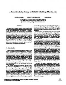
5.2. Uncertainty in Renewable Energy Sources The multi-microgrid scheduling problem has been solved by considering uncertainty in 5.2. Uncertainty in Renewable Energy Sources renewable power sources only in this section. The uncertainty for this case is shown ininFigure The multi-microgrid scheduling problem has been solved bygap considering uncertainty renewable 5a. Three cases have been considered for comparing internal and external trading, generation of in 5a. The multi-microgrid scheduling problem has been solved by considering uncertainty power sources only in this section. The uncertainty gap for this case is shown in Figure (𝑡) CGs, and charging/discharging of BESS elements. Case a is the deterministic case (Г = 0), Case renewable power sources only infor this section. The uncertainty gap fortrading, this case is 𝑚shown of in CGs, Figureand Three cases have been considered comparing internal and external generation (𝑡) = 0.5)trading, is the worst-case =considered 1), and Case is anaintermediate caseand (Г𝑚external this“section. 5a.cThree cases have(Гof been forbCase comparing generation 𝑚 (𝑡) charging/discharging BESS elements. is the internal deterministic case (Γminptq 0), Case c isofthe It can be observed from Figure 5a elements. that uncertainty for deterministic Case a (deterministic zero. (𝑡) =is0), CGs, and charging/discharging of BESS Case agap is the case (Г𝑚case) Case worst-case (Γ m ptq “ 1), and Case b is an intermediate case (Γm ptq “ 0.5) in this section. However, an uncertainty gap can be observed for Case b and even a wider gap for Case c. This (𝑡) (𝑡) c isItthe worst-case (Г = 1), and Case b is an intermediate case (Г = 0.5) in this section. 𝑚 𝑚 Case a (deterministic case) is can be observed from Figure 5a that uncertainty gap for uncertainty gap has tofrom be filled by 5a thethat CEMS through external trading (trading with utility grid), It can be observed Figure uncertainty gap for Case (deterministic case)for is zero. zero.internal However, an (trading uncertainty gap can be observed for Case b andaof even a and/or wider by gap Case c. trading among microgrids), increasing the generation CGs, utilizing However, an uncertainty gap can be observed for Case b and even a wider gap for Case c. This This BESSs. uncertainty gap has to be filled by the CEMS through external trading (trading with utility uncertainty gap has to be filled by the CEMS through external trading (trading with utility grid), grid), internal microgrids), the1–4, generation of CGs, and/or Case b:trading It can be(trading observedamong from Figure 7b that in increasing time intervals 6, and 24, uncertainty gap by internal trading (trading among microgrids), increasing the generation of CGs, and/or by utilizing has been filled by buying more power from the utility grid. Figure 8a shows that CG generation has utilizing BESSs. BESSs. been increased in the time intervals 8–11, 7b 15, that 16, and 23 tointervals fulfill the1–4, gap.6,Figure 7auncertainty shows that gap Case b: It can be observed from Figure in time and 24, Case b: It can be observed from Figure 7b that in time intervals 1–4, 6, and 24, uncertainty gap amount of by selling power haspower been reduce in time intervals 12–14 to suffice the energy needs of has has been filled buying more from the utility grid. Figure 8a shows that CG generation hasmicrogrids. been filledFigure by buying morethat power from the utility grid.in Figure 8a shows thatprice CG intervals generation has 8b shows BESSs have been charged the initial off-peak been increased in in thethe time intervals 8–11, 15, 16, and 23 to23fulfill the gap. Figure 7a shows thatand amount been increased time intervals 8–11, 15, 16, and to fulfill the gap. Figure 7a shows that discharged in the peak intervals of price. Figure 7a shows that internal trading is increased when of amount selling power haspower been reduce in time intervals to suffice to thesuffice energy needs of microgrids. of selling hasorbeen in time 12–14 intervals the energy needs CG generation is increased BESSreduce is discharged. Such type 12–14 of behavior can be observed in time of Figure 8b shows that8b BESSs have been charged in the initial in off-peak price intervals and discharged microgrids. Figure shows that BESSs have been charged the initial off-peak price intervals and in intervals 8–11, 16, 16, 23 and 15–18, respectively. thedischarged peak intervals price. Figure of 7a price. showsFigure that internal trading is increased when CG generation in theofpeak intervals 7a shows that internal trading is increased when is increased or BESSisisincreased discharged. Suchistype of behavior can be observed in can timebeintervals 8–11, 16, 16, CG generation or BESS discharged. Such type of behavior observed in time 23intervals and 15–18, respectively. 8–11, 16, 16, 23 and 15–18, respectively. b

Power (kW)

Power (kW)

a

b

a

Time (hours) Figure 7. Collective power trading: (a) Internal trading; and (b) External trading.

Case c: The uncertainty gap of Case cTime is wider than that of Case b as shown in Figure 5a. (hours) Therefore, Case c realization requires more generation or internal/external trading to assure the 7. Collective power trading: (a)scenario. Internal trading; andFigures (b) External trading. feasibility Figure ofFigure solution even inpower the worst-case 7 and 8 depict that the 7. Collective trading: (a) Internal However, trading; and (b) External trading. general behavior of Case c is similar to that of Case b. The driving force of this behavior is the Case c: Theofuncertainty Casecan c isbewider thanbythat of Case as shown in charging Figure 5a. minimization the operationgap costofwhich achieved buying from b utility grid and Case c: The uncertainty gap of Case c is wider than that of Case b as shown in Figure 5a. Therefore, Therefore, c realization requires more generation generationoforCGs internal/external to assure BESSs in Case off-peak price intervals, increasing in the mid-peaktrading price intervals, andthe Case c realization requires more generation or internal/external trading to assure the feasibility feasibility of the solution the worst-case scenario. BESS However, Figures 7 intervals. and 8 depict that the of increasing sellingeven to thein utility grid and discharging in the peak price

solution in theofworst-case Figures 8 depict the behavior general behavior generaleven behavior Case c is scenario. similar to However, that of Case b. The7 and driving force that of this is the of minimization Case c is similar tooperation that of Case The can driving force ofbythis behavior the minimization of the of the cost b. which be achieved buying from is utility grid and charging operation whichprice can be achieved by buying from utility gridinand off-peakand price BESSs incost off-peak intervals, increasing generation of CGs thecharging mid-peakBESSs price in intervals, increasing the selling to the utility grid and discharging BESS in the peak price intervals.

Energies 2016, 9, 278

13 of 21

intervals, increasing generation of CGs in the mid-peak price intervals, and increasing the selling to the utility and discharging BESS in the peak price intervals. Energies 2016,grid 9, 278 13 of 21 Energies 2016, 9, 278

13 of 21

b a

b

Power (kW)

Power (kW)

a

Time (hours) Time (hours) Figure 8. 8. (a) (a)Collective Collectivegeneration generationamount amount Controllable generators (CGs); (b) Cumulative Figure of of Controllable generators (CGs); and and (b) Cumulative state Figure 8. (a) Collective generation amount of Controllable generators (CGs); and (b) Cumulative state of charge (SOC) of battery energy storage system (BESSs). of charge (SOC) of battery energy storage system (BESSs). state of charge (SOC) of battery energy storage system (BESSs).

Power (kW) Power (kW)

5.3. Uncertainty in Electric Load 5.3.5.3. Uncertainty UncertaintyininElectric ElectricLoad Load In this section, the multi-microgrid scheduling problem has been solved by considering In Inthis problem has has been beensolved solvedbybyconsidering considering thissection, section,the themulti-microgrid multi-microgrid scheduling scheduling problem uncertainty in electric loads only. The hour-wise uncertainty gap is shown in Figure 5b. In this uncertainty uncertaintygap gapisisshown shownininFigure Figure5b. 5b.In In this uncertaintyininelectric electricloads loadsonly. only. The The hour-wise hour-wise uncertainty this section also, three cases have been considered. Case a is the deterministic case (load with nominal section also, threecases caseshave havebeen beenconsidered. considered. Case nominal section also, three Case aa is is the the deterministic deterministiccase case(load (loadwith with nominal values), Case c is the worst-case (load increased by 10%) and Case b is an intermediate case (load values), Casec is c isthe theworst-case worst-case(load (load increased increased by 10%) case (load values), Case 10%) and andCase Casebbisisan anintermediate intermediate case (load increased byby5%). The trend ofofuncertainty gap is different different from fromthat thatofofSection Section5.25.2 where, due to increased 5%). The trend uncertainty gap is where, due to to increased by 5%). The trend of uncertainty gap is different from that of Section 5.2 where, due uncertainty ininrenewable sources, uncertaintycan can be observedatat noon time. uncertaintyin renewableenergy energysources, sources, maximum maximum uncertainty thethe noon time. uncertainty renewable energy maximum uncertainty canbebeobserved observed at the noon time. However, due to the presence of load in all the time intervals the uncertainty is comparatively However, to the presence of load alltime the intervals time intervals the uncertainty is comparatively However, duedue to the presence of load in allinthe the uncertainty is comparatively uniform uniform and can from Figure 5b. uniform canbebeobserved observed from and can be and observed from Figure 5b.Figure 5b. Case b: It Itcan bebeobserved from Figure 9a that buying buying fromthe the utilitygrid grid has increased in the Case canbe observedfrom fromFigure Figure 9a 9a that that increased in in thethe Case b: b: It can observed buyingfrom from theutility utility gridhas has increased time intervals interval generation generationcost costofofMG MG 1 is lower than time intervals1–6, 1–6,and and24. 24.In Inthe themid-peak mid-peak price interval 1 is lower than thethe time intervals 1–6, and 24. In the mid-peak price interval generation cost of MG1 is lower than the market the selling sellingand andbuying buyingprices, prices,which which marketbuying buyingprice priceand andthat that of of MG MG22 lies lies between between the cancan be be market buying price and that of MG2 lies between the selling and buying prices, which can be observed observed fromFigure Figure6b. 6b.Therefore, Therefore, MG MG22 increases increases its 7–11 asas shown in in observed from its generation generationinintime timeintervals intervals 7–11 shown from Figure 6b. Therefore, MG2 increases its generation in time intervals 7–11 as shown in Figure 10a. Figure 10a.However, However,due duetotohigher higher magnitude magnitude of trading Figure 10a. of loads loads in in time timeintervals intervals19–23, 19–23,external external trading However, due to higher magnitude of loads in time intervals 19–23, external trading (buying from (buying fromutility utilitygrid) grid)has hasincreased increased in in these time MG 1 and MG 2 (buying from time intervals. intervals.In Indeterministic deterministiccase, case, MG 1 and MG 2 utility grid)tohas increased inthe these time intervals. In12–15 deterministic case, MG1 amount and MGof2 generate to generate their fullest in peak price intervals and sell the surplus power to generate to their fullest in the peak price intervals 12–15 and sell the surplus amount of power to their fullest in the However, peak pricecost intervals and sell the surplus amount of power to the utility grid. utilitygrid. grid. of CG CG12–15 in MG MG and selling thethe utility However, cost of in 33,, being being sandwiched sandwichedbetween betweenthe thebuying buying and selling However, cost of CG in MG , being sandwiched between the buying and selling prices, only generated 3 prices, onlygenerated generatedrequired requiredamount amount (neither (neither buying that external prices, only buying nor norselling). selling).Figure Figure9a9ashows shows that external required amount (neither buying nor selling). Figure 9a shows thathas external tradingand hasdischarged significantly trading has significantly reduced in the peak price intervals. BESS been charged trading has significantly reduced in the peak price intervals. BESS has been charged and discharged reduced in the intervals. BESS10b hasand beeninternal charged and discharged twice in this case as time shown twice in thispeak case price shown Figure of the twice in this case asasshown inin Figure 10b and internal trading tradinghas hasincreased increasedininmost most of the time in intervals Figure 10b internal trading as and shown in Figure 9b. has increased in most of the time intervals as shown in Figure 9b. intervals as shown in Figure 9b.

a a

b

b

Time (hours)

Time (hours) Figure Collectivepower powertrading: trading: (a) (a) Internal Figure 9.9.Collective Internal trading; trading;and and(b) (b)External Externaltrading. trading. Figure 9. Collective power trading: (a) Internal trading; and (b) External trading.

Energies 2016, 9, 278 Energies 2016, 9, 278

14 of 21 14 of 21

a Power (kW)

b

Time (hours) Figure (a)Collective Collectivegeneration generation amount amount of BESSs. Figure 10.10.(a) of CGs; CGs; and and(b) (b)Cumulative CumulativeSOC SOCofof BESSs.

Case c: c: It It is is the worst-case of all all the theMGs MGstake taketheir theirworst worstvalues. values. Figure Case the worst-casescenario, scenario,i.e., i.e. loads loads of Figure 5b5b shows that uncertainty comparedto toCase Caseb.b.The Thegeneral general trend similar shows that uncertaintygap gapisishigher higherin inthis this case case as as compared trend is is similar to to that of of Case b, b, with general trend trendofofMMG MMGisisdecided decidedbyby the market that Case withelevated elevatedmagnitudes. magnitudes. The general the market price signals and per-unit generation cost ofof CGs in in each MG. It can bebe observed from Figure 6b6b that price signals and per-unit generation cost CGs each MG. It can observed from Figure that during price interval 1 has generated maximum power 2 and MG 3 have during off-peakoff-peak price interval MG1 hasMG generated maximum power but MG2but andMG MG generated 3 have generated minimum power the anddeficit bought the deficit from the In utility grid. In the mid-peak minimum power and bought amount fromamount the utility grid. the mid-peak price intervals price intervals MG 1 and MG 2 have generated maximum and MG 3 has generated as per requirement. MG1 and MG2 have generated maximum and MG3 has generated as per requirement. BESSs are BESSs in areoff charged in off andprice mid-peak priceand intervals and in aremid usedorinon-peak mid or on-peak price intervals. charged and mid-peak intervals are used price intervals. Uncertainty bothRenewable RenewableEnergy EnergySources Sources and and Electric Electric Load 5.4.5.4. Uncertainty ininboth Load finalcase, case,the themulti-microgrid multi-microgrid scheduling scheduling problem In In thethefinal problem has hasbeen beensolved solvedbybyconsidering considering uncertainties in both renewable power sources and electric loads. The uncertainty gaps for thisfor case uncertainties in both renewable power sources and electric loads. The uncertainty gaps this areare shown in in Figure 6a.6a. Similar to to previous sections, in in this section also, three cases have been case shown Figure Similar previous sections, this section also, three cases have been considered. Case is the deterministic Case is the worst-case = 2), 𝑚 (𝑡) 𝑚 (𝑡) ptq “ = “ 2), considered. Case a isa the deterministic casecase (Γm(Г 0),0), Case c isc the worst-case (Γm(Гptq andand Case Case b is an intermediate case (Г𝑚 (𝑡) = 1). There are two sets of random variables in this case. One b is an intermediate case (Γm ptq “ 1). There are two sets of random variables in this case. One set is set is associated with the load and other with the renewable power sources. The general trend of associated with the load and other with the renewable power sources. The general trend of uncertainty uncertainty gap shown in Figure 6a reflects the behavior of both of the previous cases. gap shown in Figure 6a reflects the behavior of both of the previous cases. 5.4.1. Grid-Connected Mode 5.4.1. Grid-Connected Mode Case b: The value of budget of uncertainty (Г (𝑡)) is set to one in this case which makes the Case b: The value of budget of uncertainty (Γ𝑚 m ptq) is set to one in this case which makes the optimization problem to select one of the two (load and renewable power) uncertainties at each optimization problem to select one of the two (load and renewable power) uncertainties at each time time interval t. In order to assure the feasibility of solution under all possible realizations, instead of interval t. In order to assure the feasibility of solution under all possible realizations, instead of selecting randomly, the proposed algorithm has been set to select the worst value. Generally, due to selecting proposed algorithm has been set to select the worst Generally, due to higher randomly, magnitude the of load as compared to renewable power generation, loadvalue. uncertainty is higher higher magnitude of load as compared to renewable power generation, load uncertainty is higher and is selected by the optimization algorithm. However, in the time intervals 10–14 the uncertainty and selected by the optimization algorithm. However, in the time intervals uncertainty of ofisrenewable sources is at the peak and is higher than the uncertainty of load10–14 in thethe corresponding renewable sources is at the peak and is higher than the uncertainty of load in the corresponding time intervals. Therefore, renewable power uncertainty has been considered by the RO algorithm time in intervals. Therefore, power uncertainty been considered by the time RO algorithm these time intervalsrenewable and load uncertainty has been has considered in the remaining intervals. in these time intervals and load uncertainty remaining intervals. The difference between Case ahas andbeen Caseconsidered b, as shownininthe Figure 11a, is time identical to that of Case c difference between Case a 9a, andinCase b, asintervals shown in Figure 11a, is generation identical toamounts that of Case in The Section 5.3, as shown in Figure the time 1–6 and 24. The of in time 7–11 19–23 alsotime identical to those of Case in Figure 10a. However, c inCGs Section 5.3,intervals as shown in and Figure 9a, are in the intervals 1–6 and 24. cThe generation amounts of theinmagnitude of reduction in19–23 sellingare power time intervals in Figure 11a is10a. identical to thatthe CGs time intervals 7–11 and also in identical to those11–13 of Case c in Figure However, of Case c of inreduction Figure 7a.inBehavior of BESSincharging/discharging that of Figure to 10b as of magnitude selling power time intervals 11–13isinsimilar Figureto 11a is identical that shown in Figure 12b. Case c in Figure 7a. Behavior of BESS charging/discharging is similar to that of Figure 10b as shown in Figure 12b.

Energies 2016, 9, 278 Energies 2016, 9, 278 Energies 2016, 9, 278

15 of 21 15 of 21 15 of 21

Power Power(kW) (kW)

a a

b b

Time (hours) Time (hours)

Figure 11.11. Collective power trading grid (a) Internaltrading; trading; and(b) (b) External trading. Figure Collective power tradingin gridconnected connected mode: External trading. Figure 11. Collective power trading iningrid connected mode: (a) Internal Internal trading;and and (b) External trading.

a a Power Power(kW) (kW)

b b

Time (hours) Time (hours) Figure 12. Grid-connected mode: (a) Collective generation amount of CGs; and (b) Cumulative SOC Figure (b) Cumulative Cumulative SOC SOC Figure 12. 12. Grid-connected Grid-connected mode: mode: (a) (a) Collective Collective generation generation amount amount of of CGs; CGs; and and (b) of BESSs. of of BESSs. BESSs.

is the worst possible case in the given framework of simulations. In this case, both of c: Case Case c: This This is the the worst worst possible possible case case in in the the given given framework framework of of simulations. simulations. In In this this case, case, both both thethe random variables sets (load and renewable generators) are assumed to take their worst values in of random variables sets (load and renewable generators) are assumed to take their worst of the random variables sets (load and renewable generators) are assumed to take their worst each time interval t. It can be observed from Figure 6a that theFigure uncertainty gap is summation of Caseisc values values in in each each time time interval interval t. t. It It can can be be observed observed from from Figure 6a 6a that that the the uncertainty uncertainty gap gap is of Figure 5a of and Case c of Figure5a5b. Due to the absence of renewable energy sources (PV andenergy CS) in summation Case c of Figure and Case c of Figure 5b. Due to the absence of renewable summation of Case c of Figure 5a and Case c of Figure 5b. Due to the absence of renewable energy the time (PV intervals 1–7 and 19–24 the uncertainty gap adjustment trend is similar to that of Section 5.3. sources and CS) in the time intervals 1–7 and 19–24 the uncertainty gap adjustment trend sources (PV and CS) in the time intervals 1–7 and 19–24 the uncertainty gap adjustment trend is is However, inthat the remaining time intervals due to combined uncertaintiesintervals of both the random variable similar similar to to that of of Section Section 5.3. 5.3. However, However, in in the the remaining remaining time time intervals due due to to combined combined sets, the trend isboth differentrandom from other two cases explainedisindifferent Sections 5.2 and 5.3. Unlike to the other uncertainties uncertainties of of both the the random variable variable sets, sets, the the trend trend is different from from other other two two cases cases explained explained two cases, selling power has reduced to zero in time intervals 11–15, as shown in Figure 11a. Similarly, in Sections 5.2 and 5.3. Unlike to the other two cases, selling power has reduced to zero in Sections 5.2 and 5.3. Unlike to the other two cases, selling power has reduced to zero in in time time in both of 11–15, the previous casesin explained in Sections 5.2 and 5.3 internal trading hascases been progressively intervals as shown Figure 11a. Similarly, in both of the previous explained intervals 11–15, as shown in Figure 11a. Similarly, in both of the previous cases explained in in increased5.2 from Case ainternal to Case trading c, but Figure 11b shows that internal trading has Case decreased in Case cbut in Sections and 5.3 has been progressively increased from a to Case c, Sections 5.2 and 5.3 internal trading has been progressively increased from Case a to Case c, but comparisonshows with Case b.internal This behavior ishas due to the factinthat in Case comparison c due to uncertainty in both of Figure Figure 11b 11b shows that that internal trading trading has decreased decreased in Case Case cc in in comparison with with Case Case b. b. This This the random variable setsfact surplus amount of individual MGs hasindrastically reduced. behavior is due to the that in Case c due to uncertainty both of the random variable sets behavior is due to the fact that in Case c due to uncertainty in both of the random variable sets surplus amount of surplus amountMode of individual individual MGs MGs has has drastically drastically reduced. reduced. 5.4.2. Islanded

5.4.2. Islanded Mode objective of the islanded mode operation is to minimize both the operation cost and amount 5.4.2.The Islanded Mode of load shedding. However, due to the finite capacities to of power sources, load operation shedding mightand be The The objective objective of of the the islanded islanded mode mode operation operation is is to minimize minimize both both the the operation cost cost and unavoidable in some cases. It can be observed from Figure 13a that even for the deterministic case amount amount of of load load shedding. shedding. However, However, due due to to the the finite finite capacities capacities of of power power sources, sources, load load shedding shedding (Γ 0),unavoidable there is some unavoidable load shedding at time from intervals 18 and 19. The generation m ptq = might be in some cases. It can be observed Figure 13a that even might be unavoidable in some cases. It can be observed from Figure 13a that even for for the the amount of CGs shown in Figure 14a is different from the grid-connected case, i.e., Figure 12a. The case (𝑡) deterministic == 0), there is some unavoidable load shedding at time intervals 18 and 19. (𝑡) deterministic case case (Г (Г𝑚 0), there is some unavoidable load shedding at time intervals 18 and 19. with SOC of BESSs is𝑚the of same. BESSs have been used more efficiently inthe islanded mode to minimize The generation amount CGs shown in Figure 14a is different from grid-connected case, The generation amount of CGs shown in Figure 14a is different from the grid-connected case, i.e. i.e. the amount of load shedding. Figure 12a. The case with SOC of BESSs is the same. BESSs have been used more efficiently Figure 12a. The case with SOC of BESSs is the same. BESSs have been used more efficiently in in islanded islanded mode mode to to minimize minimize the the amount amount of of load load shedding. shedding.

Energies 2016, 9, 278

16 of 21 16 of 21 16 of 21

Power(kW) (kW) Power

Shedload load(kW) (kW) Shed

Energies 2016, 9, 278 Energies 2016, 9, 278

a a

b b

Time (hours) Time (hours) Figure 13. Islanded mode: (a) Collective amount of load shed; and (b) Internal trading.

Figure 13. Islanded mode: (a)(a)Collective load shed; Internal trading. Figure 13. Islanded mode: Collective amount amount ofofload shed; andand (b) (b) Internal trading.

b b

Power(kW) (kW) Power

a a

Time (hours) Time (hours) Figure 14. Islanded mode: (a) Collective generation amount of CGs; and (b) Cumulative SOC of BESSs. Figure 14. Islanded mode: (a) Collective generation amount of CGs; and (b) Cumulative SOC of BESSs.

Figure 14. Islanded mode: (a) Collective generation amount of CGs; and (b) Cumulative SOC of BESSs. Case b: In this case, one of the two uncertainties will be selected by the optimization algorithm Case b: In this case, one of the two uncertainties will be selected by the optimization algorithm and scheduling will beone carried outtwo for the worst case inwill the given frame of Amount of Case b: In this case, of the uncertainties selected byuncertainties. the optimization algorithm and scheduling will be carried out for the worst case in the be given frame of uncertainties. Amount of load shedding has been increased in this case as compared to the deterministic case. It can be and scheduling willhas be carried out for in thethis worst in the given frame of uncertainties. Amount of load shedding been increased case case as compared to the deterministic case. It can be observed from Figure 13a and 14b that load shedding has been carried out only in the peak load observed has frombeen Figure 13a and in 14b that load shedding hastobeen carried out only in the peak load load shedding increased this case as compared the deterministic case. It can be observed intervals after utilizing BESSs. The dynamics of BESSs charging/discharging are also changing more intervals after utilizing BESSs. The dynamics of BESSs charging/discharging are also changing more from Figure 13a 14b that shedding has frequently asand compared to load the deterministic case.been carried out only in the peak load intervals after frequently as compared to the deterministic case. utilizing BESSs. dynamics charging/discharging areand alsoload) changing more frequently as Case c: The In this case, bothof ofBESSs the uncertainties (renewable power have been considered Case c: In this case, both of the uncertainties (renewable power and load) have been considered by thetooptimization algorithm for scheduling of the MMG system. Amount of load shedding in the compared the deterministic case. by the optimization algorithm for scheduling of the MMG system. Amount of load shedding in the peak c: price intervals further in this (renewable case. Due to the consideration uncertainties in In this case,has both of theincreased uncertainties and load)of have been considered Case peak price intervals has further increased in this case. Due to power the consideration of uncertainties in both renewable energy sources and electric loads, internal trading has been reduced in this case in by theboth optimization algorithm for and scheduling of the MMGtrading system. of load shedding renewable energy sources electric loads, internal hasAmount been reduced in this case in in the comparison with previous cases. Figure 14a depicts that CGs outputs have been increased to fulfill peak price intervals further increased in depicts this case. the consideration of uncertainties in comparison withhas previous cases. Figure 14a thatDue CGs to outputs have been increased to fulfill the load demands. Load shedding has been carried out only in those time intervals where, both the load demands. Load shedding has been carried out only in those time intervals where, both both renewable energy sources and electric loads, internal trading has been reduced in this case in CGs and BESSs were unable to fulfill the electric load demands of the MMG system. CGs and BESSs were unable toFigure fulfill the load demands of the MMG system. comparison with previous cases. 14aelectric depicts that CGs outputs have beenminimize increased fulfill the The general behavior in all the cases to minimize the operation cost and thetoload The general behavior in all the cases to minimize the operation cost and minimize the load load demands. Load shedding has been carried out only in those time intervals where, both CGs and shedding of the MMG system can be summarized as follows. shedding of the MMG system can be summarized as follows. BESSs were unable to fulfill the electric load demands of the MMG system. 𝐶𝐺 𝐶𝐺 (𝑡)) 𝑆𝐸𝐿𝐿 𝐵𝑈𝑌  When 𝑃𝑈𝐶𝑚,𝑔 𝐶𝐺 (𝑝𝑚,𝑔 𝐶𝐺 (𝑡)) < 𝐶 𝑆𝐸𝐿𝐿 (𝑡) < 𝐶 𝐵𝑈𝑌 (𝑡), CG generates to its fullest, sends to other MGs  general When 𝑃𝑈𝐶 utility , CG generates minimum power and either 𝑚,𝑔 (𝑝 𝑚,𝑔 (𝑡)) ´ ¯𝐶 CGs or receives from other MGs having cheaper buys from the utility grid. SELL CG CG BUY receives from other MGs having cheaper CGs or buysCG fromdoes the utility grid. ptq ďmainly PUCm,g ‚ When C is charged pm,g ptq < C priceptq, not involve in external  BESS in off-peak/mid-peak intervals and discharged in the peak intervals. trading.  BESS is charged mainly in off-peak/mid-peak price intervals and discharged in the peak intervals. Itsuffices its trading local load demands andBESS mayissend to other having expensive CGs. MGs Internal is increased when discharged or MGs generation of CGs in individual ´ ¯  Internal trading is increased when BESS is discharged or generation of CGs in individual MGs CG CG BUY SELL is increased. ptq ą C ptq, CG generates minimum power and either ‚ Whenis PUC m,g pm,g ptq ě C increased.

‚ ‚

receives from other MGs having cheaper CGs or buys from the utility grid. BESS is charged mainly in off-peak/mid-peak price intervals and discharged in the peak intervals. Internal trading is increased when BESS is discharged or generation of CGs in individual MGs is increased.

Energies 2016, 9, 278 Energies 2016, 9, 278 

17 of 21 17 of 21 

Energies 2016, 9, 278  17 of 21   Energies 2016, 9, 278  Load  shedding  is  carried  out  only  in  peak  load  intervals  when  both  CGs  and  BESSs  were  ‚ Load shedding is carried out only in peak load intervals when both CGs and BESSs were unable unable to fulfill the electric load demands of the MMG system.   to Load  is load carried  out   only  Load  in shedding  peak  load  is intervals  carried  out  when  only  both  in  peak  CGs  and  load BESSs  intervals  were  when  both  CGs  and  B fulfillshedding  the electric demands of the MMG system. unable to fulfill the electric load demands of the MMG system.  unable to fulfill the electric load demands of the MMG system.  5.5. Operation Cost and Budget of Uncertainty  5.5. Operation Cost and Budget of Uncertainty Various values of budget of uncertainty (Г ) and probability of unfeasible solution (ԑ ) in the  5.5. Operation Cost and Budget of Uncertainty  5.5. Operation Cost and Budget of Uncertainty  Various values of budget of uncertainty (Γm ptq) and probability of unfeasible solution (εe ) in the given uncertainty bounds have been compared against the daily operation cost of the MMG system in  Various values of budget of uncertainty (Г Various values of budget of uncertainty (Г ) and probability of unfeasible solution (ԑ ) and probability of unfeasible solutio given uncertainty bounds have been compared against the daily operation cost of the MMG ) in the  system in both operation modes. It can be observed from Table 2 that operation cost for uncertain load is higher  given uncertainty bounds have been compared against the daily operation cost of the MMG system in  given uncertainty bounds have been compared against the daily operation cost of the MM both operation modes. It can be observed from Table 2 that operation cost for uncertain load is higher as  compared  to  the  corresponding  uncertainty  in  renewable  power,  which  is  due  to  the  absence  of  both operation modes. It can be observed from Table 2 that operation cost for uncertain lo as both operation modes. It can be observed from Table 2 that operation cost for uncertain load is higher  compared to the corresponding uncertainty in renewable power, which is due to the absence of solar related renewable power in the morning and night times. Corresponding grid‐connected mode  as  compared  to  the  corresponding  as uncertainty  compared  to  in the  renewable  corresponding  power,  uncertainty  which  is  due  in  to  renewable  the  absence  power,  of  which  is  due  to  the solar related renewable power in the morning and night times. Corresponding grid-connected mode operation cost has been used as a reference for calculating increase percentage in each case.  solar related renewable power in the morning and night times. Corresponding grid‐connected mode  solar related renewable power in the morning and night times. Corresponding grid‐conn operation cost has been used as a reference for calculating increase percentage in each case. operation cost has been used as a reference for calculating increase percentage in each case.  operation cost has been used as a reference for calculating increase percentage in each case

Table 2. Performance in grid‐connected mode with single source of uncertainty.  Table 2. Performance in grid-connected mode with single source of uncertainty. Table 2. Performance in grid‐connected mode with single source of uncertainty.  Table 2. Performance in grid‐connected mode with single source of uncertainty.  Uncertainty in Electric Load Budget of Uncertainty and Error  Uncertainty in Renewable Power Budget of Uncertainty and Error Budget of Uncertainty Uncertainty Power Uncertainty in Renewable Power Uncertainty Inc.  Cost in  Electric Load Inc.  Cost  in Renewable Uncertainty in Electric Load Uncertainty in El Budget of Uncertainty and Error  Uncertainty in Renewable Power and Error    Г ԑ   Г   1)  (M ₩ (%age)  (M ₩)  (%age)  Inc.  Cost    Inc.  Inc.  Cost    Cost  Cost  řT Cost Inc. Cost Inc.   ptq   Г Γm ԑ ε  e Г ԑ   Гt“1 Γ m Г   ptq   1)  1)  (M ₩ (%age)  (M ₩ (M ₩)  (%age)  (%age)  (M ₩)  (M ) (%age) (M ) (%age) 0  0  0.58  1.53574  0  1.53574  0  0  0 0.58  0  1.53574  0  0.58  1.53574  1.53574  1.53574  0.25  6 0  0 0.15  1.55641  1.34  1.58472  3.10  0.58 1.53574 00  1.53574 0 0 0  0.25  6  0.15  0.25  1.55641  6  0.15  1.34  1.55641  1.58472  3.10  1.34  1.58472  0.5  0.25 12  6 0.012  1.57720  2.71  1.63419  0.15 1.55641 1.34 1.58472 3.10 6.42  −4 0.5  12  0.012  0.5  1.57720  12  0.012  2.71  1.57720  1.63419  6.42  2.71  1.63419  0.5 12 0.012 1.57720 2.71 1.63419 6.42 1.59820  4.08  1.68384  9.66  0.75  18    2.6 × 10 −4´4 −4 1.59820 4.08 1.68384 9.66 2.6 ˆ 10 1.59820  4.08  1.59820  1.68384  9.66  4.08  1.68384  0.75 0.75 18  18 0.75  18  2.6 × 10−6  2.6 × 10   ´6 1.61913  5.44  1.73342  1  24  24 1.3 × 10 1 1.61913 5.44 1.73342 12.89 12.89  1.3 ˆ 10 −6  1.61913  5.44 −6  1.61913  1.73342  12.89  5.44  1.73342  1  24  24  1.3 × 10   1  1.3 × 10 1 ₩ is Korean Won.  is Korean Won. Energies 2016, 9, 278  17 of 21  1Energies 2016, 9, 278  1  ₩ is Korean Won.   ₩ is Korean Won. 

. The  Table 3 shows that amount of load shedding increases with increase in the value of Г ptq. when  both  CGs  a Table 3 shows amount of load increases with increase inin the value of Γm were  . The  Table 3 shows that amount of load shedding increases with increase in the value of Г Table 3 shows that amount of load shedding increases with increase in the value of Load that shedding  is  carried  out  shedding only  Load  in  shedding  peak  load is intervals  carried  out  when  only  both  CGs  peak  and  load  BESSs  intervals  operation  cost  of  the  islanded  mode  is  always  greater  than  that  of  corresponding  grid‐connected  The operation cost the islanded mode always greater than that corresponding grid-connected unable to fulfill the electric load demands of the MMG system.  unable to fulfill the electric load demands of the MMG system.  operation  cost  of of the  islanded  mode  operation  is is always  cost  of  greater  the  islanded  than  that  mode  of of corresponding  is  always  greater  grid‐connected  than  that  of  corresponding  grid mode.  The  two  factors  that  result  this  increase  are  heavy  penalty  costs  for  shedding  loads  and  mode.  The  two  factors  result  mode.  this  The  increase  two  factors  are  heavy  that penalty  result  costs  increase  for  shedding  are  heavy  loads  and  costs  for  shedding mode. The two factors thatthat  result this increase are heavy penalty coststhis  for shedding loads and penalty  inability inability of the MMG system to trade with the utility grid.  5.5. Operation Cost and Budget of Uncertainty  5.5. Operation Cost and Budget of Uncertainty  inability of the MMG system to trade with the utility grid.  inability of the MMG system to trade with the utility grid.  of the MMG system to trade with the utility grid. Table  4 4 shows  the  operation  cost  considering  uncertainties  in  both  renewable  power  sources  Table  shows  operation  Table  4  Various values of budget of uncertainty (Г shows  the  operation  cost  considering  uncertainties  cost  both  considering  renewable  uncertainties  power  sources  in  both  renewable  pow Various values of budget of uncertainty (Г ) and probability of unfeasible solution (ԑ ) and probability of unfeasible sol ) in the  Table 4 shows thethe  operation cost considering uncertainties inin  both renewable power sources and and  loads.  It  can  be  observed  that  the  operation  cost  at  Г   =  1  is  higher  than  both  of   the  and  It loads.  It observed can  be  observed  that  and  loads.  the given uncertainty bounds have been compared against the daily operation cost of the  operation  It  can  cost  observed  at  Г that  the  operation  cost  at  Г   =  1  is  higher  than  both  of  the  =  1  is  higher  than  b ptq loads. cangiven uncertainty bounds have been compared against the daily operation cost of the MMG system in  be that the operation cost at Γbe  = 1 is higher than both of the operation cost m operation cost in Table 1 at  ГГ operation cost in Table 1 at    = 1 which is due to the consideration of worst scenario. The case  = 1 which is due to the consideration of worst scenario. The case  operation cost in Table 1 at  Г     = 1 which is due to the consideration of worst scenar both operation modes. It can be observed from Table 2 that operation cost for uncertain load is higher  both operation modes. It can be observed from Table 2 that operation cost for uncertai in Table 1 at Γm ptq = 1 which is due to the consideration of worst scenario. The case with amount of with amount of load shedding is the same. However, probability of error has increased at  = 1  as  compared  to  the  corresponding  as uncertainty  compared  to  in has the  renewable  corresponding  power,  which  uncertainty  due  in to  renewable  the  with amount of load shedding is the same. However, probability of error has increased at  with amount of load shedding is the same. However, probability of error has increased a Г Гabsence  = 1 power,  ptq = is  load shedding is the same. However, probability of error increased at Γm 1 due to inclusion ofof  which  is  due  to due to inclusion of more random variables.  solar related renewable power in the morning and night times. Corresponding grid‐connected mode  solar related renewable power in the morning and night times. Corresponding grid‐c due to inclusion of more random variables.  due to inclusion of more random variables.  more random variables.

operation cost has been used as a reference for calculating increase percentage in each case.  operation cost has been used as a reference for calculating increase percentage in each  Energies 2016, 9, 278  17 of 21  Table 3. Performance in islanded mode with single source of uncertainty.  Table 3. Performance in islanded mode with single source of uncertainty.  Table 3. Performance in islanded mode with single source of uncertainty.  Table 3. Performance in islanded mode with single source of uncertainty.

Energies 2016, 9, 278 

Table 2. Performance in grid‐connected mode with single source of uncertainty.  Table 2. Performance in grid‐connected mode with single source of uncertaint  Load  shedding  is  carried  out  only   in  Load  peak  shedding  load  intervals  is  carried  when  out both  only CGs  in  peak  and  BESSs  load  intervals  were  when  both  CGs  an Budget of Uncertainty and  Budget of Uncertainty and  Budget of Uncertainty and  Uncertainty in Renewable Power  Uncertainty in Renewable Power  Uncertainty in Electric Load  Uncertainty in Elect Uncertainty in Renewable Power  Uncertainty in Electric Load  Budgetunable to fulfill the electric load demands of the MMG system.  of Uncertainty and Error Uncertainty in Renewable Power Uncertainty in Electric Load unable to fulfill the electric load demands of the MMG system.  Uncertainty in Electric Load Uncertainty  Budget of Uncertainty and Error  Budget of Uncertainty Uncertainty in Renewable Power and Error  Uncertainty in Renewable Power Error  Error  Error  Inc.    Inc.  Inc.  Cost  Cost  Cost  řT Shed Load Cost Inc. Load Shed Cost Inc. Shed Load  Cost  Inc.  Load Shed Cost      Inc.  Inc. Inc. Load Shed Cost     Inc.  Cost    Γm ԑptq  Г εe  Shed Load       Г Cost  ԑ Load Shed     Shed Load  Γ   ptq Г Г t“1 1)  Г ԑ (kWh) ԑ)1)  Г (%age) ГCost  5.5. Operation Cost and Budget of Uncertainty  (M ₩ (%age)  (M ₩ (M ₩)  (%age)  (%age)  (M ₩)  (M (kWh) (M ) (%age) Г Г   m5.5. Operation Cost and Budget of Uncertainty  ԑ   Г (kWh)  (M ₩ (%age)  (kWh)  (M ₩)  )  (%age)  (M ₩)  (kWh)  (M ₩) )  (%age) (kWh)  (kWh)  (M ₩ (M ₩) (%age)  (%age)  (kWh)  0  0 0  0.58 0.58  66 0  1.53574 0  0.58  0  66 1.53574  0  0  1.53574  0 1.57458 2.53 1.57458 2.53 0  0  0.58  66  0  0  1.57458  0.58  2.53  66  66  1.57458  1.57458  2.53  2.53  66  1.57458  Various values of budget of uncertainty (Г Various values of budget of uncertainty (Г ) and probability of unfeasible solution (ԑ ) and probability of unfeasible solu ) in the  0  0 0.25  0.58  66 0.15  1.57458  1.57458  2.53  0.25  1.55641 6  2.53  0.15  1.34 15066  1.55641  1.58472  3.10  1.34  1.58472  6 0.15 6  0.15 1.59611 3.93 1.63200 6.27 0.25 0.25 6  74  0.25  74given uncertainty bounds have been compared against the daily operation cost of the M 6 1.59611  0.15  3.93  74  150  1.63200  6.27  150  1.63200  given uncertainty bounds have been compared against the daily operation cost of the MMG system in  0.25  150  1.59611  1.63200  3.93  0.012 84 0.5 1.59611  1.57720 12  3.93  0.012  2.71 248 1.57720  1.63419  6.42  2.71  1.63419  0.5 6  0.5  12 0.15 12  0.012 74  1.61778 5.34 1.69128 10.136.27  0.5  both operation modes. It can be observed from Table 2 that operation cost for uncertain load is higher  12  0.012  84 0.5  −4 both operation modes. It can be observed from Table 2 that operation cost for uncertai 12  1.61778  0.012  5.34  84  248  1.61778  1.69128  5.34  10.13  248  1.69128  ´4 −4 0.5  0.75 12 0.75  18 0.012 18  84  100 1.61778  248  1.69128  13.9910.13  1.64007 6.79 2.6 × 10 1.75064 2.6 ˆ 10 2.6 × 10 1.59820 18 −4 5.34  4.08 346 1.59820  1.68384  9.66  4.08  1.68384    0.75    −4 ´6 100  1.64007  6.79  100  346  1.64007  1.75064  6.79  13.99  346  1.75064  0.75 as  18  0.75  18  −4 compared  to  the  corresponding  uncertainty  as  compared  in  renewable  to  the  corresponding  power,  which  uncertainty  is  due  to  in  the  renewable  power,  which  is  due  to absence  of      2.6x10 2.6x10 1.66271 8.23 445 1.81058 1.3 ˆ 10 100  117 −6 1.75064  17.9013.99  0.75  1 18  1  242.6x1024    1.61913 24 −6 6.79  1.3 × 10 5.44  −6346  1.61913  1.73342  12.89  5.44  1.73342  1 1.64007    1.3 × 10  solar related renewable power in the morning and night times. Corresponding grid‐c −6 solar related renewable power in the morning and night times. Corresponding grid‐connected mode  1  24  24  117 1  1.66271 1.3x10  8.23  117  445  1.66271  1.81058  8.23  17.90  445  1.81058  1.3x10−6   1 ₩ is Korean Won.  1 ₩ is Korean Won.  1  operation cost has been used as a reference for calculating increase percentage in each case.  24  117  1.66271  8.23  445  1.81058  17.90  1.3x10   operation cost has been used as a reference for calculating increase percentage in each c

Table 4. Performance in both grid-connected and islanded modes with both uncertainty sources. . The  Table 3 shows that amount of load shedding increases with increase in the value of Г Table 3 shows that amount of load shedding increases with increase in the valu Table 4. Performance in both grid‐connected and islanded modes with both uncertainty sources.  Table 4. Performance in both grid‐connected and islanded modes with both uncertainty sou Table 2. Performance in grid‐connected mode with single source of uncertainty.  Table 2. Performance in grid‐connected mode with single source of uncertainty Table 4. Performance in both grid‐connected and islanded modes with both uncertainty sources.  operation  cost  of  the  islanded  mode  operation  is  always  cost greater  of  the  islanded  than  that mode  of  corresponding  is  always  greater  grid‐connected  than  that  of  corresponding  Budget of Uncertainty and Error  Budget of Uncertainty and Error  Grid‐Connected Mode Grid‐Connected Mode Islanded Mode  Islanded Mode Budget Uncertainty and Error Grid-Connected Mode Islanded Mode mode. ofThe  two  factors  that  result  mode.  this  The  increase  two are  factors  heavy  that  penalty  result  costs  this  increase  for  shedding  are  heavy  loads penalty  and  costs  for  shed Uncertainty in Electric Load Uncertainty i Budget of Uncertainty and Error  Uncertainty in Renewable Power Budget of Uncertainty and Error  Uncertainty in Renewable Power Budget of Uncertainty and Error  Grid‐Connected Mode Islanded Mode  Inc.  Shed Load  Cost    Inc.  Inc.  Shed Load  Cost    Cost  Cost  Inc.  Cost    Inc.  Inc.  Cost    Cost  Cost  Г ԑ   Г ԑ     inability of the MMG system to trade with the utility grid.   inability of the MMG system to trade with the utility grid.  Гř T Г Cost Inc. Shed Load Cost Inc. Inc.  Cost    (%age)  Inc.  (kWh)  Cost      Г Γm ptq Г(M ₩)  ԑ Shed Load    Г Γm  ptq ԑ   ԑ  εe Г(%age)    (kWh)  (M ₩)  (M ₩)  (%age)  (M ₩)  1 1 t“1 Г   Г 4  shows  the  operation  cost  (M ₩ (%age)  (M ₩)  (M ₩ (%age) (%age)  (M ₩)  (M ) )  4  shows  (%age) (kWh) (M ) )  (%age) Table  Table  the  operation  considering  uncertainties  in cost  both  considering  renewable  uncertainties  sources in  both  renewable (M ₩)  (%age)  (M ₩) power  (%age)  0  0  0  0  0.56 0.58  0  1.53574  0  0  0.56 0  0.58  (kWh)  66  1.53574  1.57458  0 2.53  66  1.57458  0 1.53574 1.53574  0  1.53574  1.53574  0  at of  0  the   =  1  is  1.53574  and  loads.  It  can  be  observed  that  and  the  loads.  operation  It  can  be  cost  observed  at  Г that  the  operation  cost  Г   =  1  is  higher  than  both  higher  th 0 0 0.56 0 66 1.57458 2.53 0 0.5  0  0.56  1.53574  0  66 1.63504  1.57458 6.07  2.53  12  6  0.056  0.5  1.63504  12  6.07  0.056  248  1.69200  10.16  248  1.69200  0.25  0.15  0.25  1.55641  6  1.34  0.15  1.58472  1.55641  3.10  1.34  1.58472  0.5 12 0.056 1.63504 6.07 248 1.69200 10.16 operation cost in Table 1 at  Г operation cost in Table 1 at  Г   = 1 which is due to the consideration of worst scenario. The case    = 1 which is due to the consideration of worst sce −4 −4 0.5 1  0.5  12  0.056  1.63504  6.07 2.71  248 1.73501  1.69200 12.98  10.16  446  1.81187  17.98  1.81187  24  12 24 4.5 × 10 1  1.73501  24  0.012  0.5  1.57720  12  12.98  0.012  1.63419  1.57720  6.42  2.71  446  1.63419    10´4   4.5 × 10 1 1.73501 12.98 446 1.81187 17.98 4.5 ˆ with amount of load shedding is the same. However, probability of error has increased at  with amount of load shedding is the same. However, probability of error has increas Г = 1  −4 −4 ´6 −4 −6 −6 1.73501  12.98  446  1.81187  17.98  1 1.5 0.75  1.5 24  1.77778 15.76 484 1.86143 21.21 2.2 ˆ 10   1.59820  4.08  1.68384  1.59820  9.66  4.08  1.68384  18 36 4.5 × 10 0.75  18  36  1.5  36  1.77778  15.76  484  1.77778  1.86143  15.76  21.21  484  1.86143    2.6 × 10 2.2 × 10 2.2 × 102.6 × 10    ´12 due to inclusion of more random variables.    due to inclusion of more random variables.  2 48 1.82185 18.63 541 1.91449 24.66 5.8−12 ˆ 10 −6 −6 −6 −12 1.5 2  1  36  1.77778  15.76  1.86143 18.63  21.21  5.44  1.73342  1.61913  12.89  5.44  541  1.73342  1 1.61913  24  18.63  2.2 × 10      2  1.82185   484  1.3 × 10 1.3 × 10 541  1.82185  1.91449  24.66  1.91449  48  24  48    5.8 × 10 5.8 × 10 −12 1 1 Table 3. Performance in islanded mode with single source of uncertainty.  Table 3. Performance in islanded mode with single source of uncertainty.  1.82185  18.63  541  1.91449  24.66  2  48   ₩ is Korean Won.   ₩ is Korean Won.  5.8 × 10  

Budget of Uncertainty and  Budget of Uncertainty and  . The  Table 3 shows that amount of load shedding increases with increase in the value of Г Table 3 shows that amount of load shedding increases with increase in the valu Uncertainty in Renewable Power  Uncertainty in Renewable Power  Uncertainty in Electric Load  Uncertainty in E Error  Error  operation  cost  of  the  islanded  mode operation  is  always cost  greater  of  the  than  islanded  that  of mode  corresponding  is  always grid‐connected  greater  than  that  of  corresponding  Shed Load  Cost  Inc.  Shed Load  Load Shed Cost  Cost    Inc.  Inc.  Load Shed Co mode.  that  mode.  are  factors  that  result  costs  this  for increase  shedding  are  loads  heavy  and  penalty  costs  for  shedd   two  factors    The  two  Г The  ԑ   result  this  Г increase  ԑ   penalty  Г Г heavy  (kWh)  (M ₩ )  (%age)  (kWh)  (kWh)  (M ₩ (M ₩)  )  (%age)  (%age)  (kWh)  (M  inability of the MMG system to trade with the utility grid.  inability of the MMG system to trade with the utility grid. 

Energies 2016, 9, 278

18 of 21

6. Conclusions An RO-based algorithm has been proposed for day-ahead scheduling of multi-microgrids in grid-connected mode. Instead of using a hard-to-obtain probability distribution of the uncertain data, a deterministic uncertainty set (upper and lower bounds) has been used in this formulation. Simulation results have proved that the developed MILP-based model is capable of providing guaranteed immunity in contrast to probabilistic guarantee of stochastic optimization techniques against the worst-case scenario: maximum uncertainty in both renewable power source and load. The developed model can be easily implemented using commercial optimization tools and it remains tractable even for large systems. The behavior of the simulation results shows that the objective of the proposed strategy is to reduce the operation cost of the MMG system in grid-connected mode and minimize load shedding while reducing operation cost in islanded mode. The unit commitment status of CGs and BESSs determined in each case remains valid even if the load and/or renewable power outputs fluctuate with the determined bounds of uncertainties. It can be concluded form the simulation results that the probability of unfeasible solution reduces drastically as the budget of uncertainty increases. Therefore, a trade-off can easily be obtained by the decision makers. The increase in operation cost in islanded mode is due to penalties for load shedding and inability of the MMG system to trade with utility grid. Simulation results depict the required units of power sources to be committed, in order to assure the proper operation of MMG system under the given uncertainty. Acknowledgments: This work was supported by Incheon National University Research Grant in 2013. Author Contributions: The paper was a collaborative effort between the authors. The authors contributed collectively to the theoretical analysis, modeling, simulation, and manuscript preparation. Conflicts of Interest: The authors declare no conflict of interest.

Nomenclature Identifiers and Binary Variables t m, n g k sm,g ptq sum,g ptq , sdm,g ptq f gm ptq , tgm ptq r f m ptq , stm ptq pvm ptq , wtm ptq csm ptq , um ptq cm ptq , dm ptq

Index of time, running from 1 to T. Index of microgrids, running from 1 to M and 1 to N, respectively. Index of dispatchable generators, running from 1 to G. Number of random variables. Commitment status identifier of dispatchable generator g of MG m at t. Start-up and shut-down identifiers of dispatchable generator g of MG m at t. External trading identifiers buying and selling (from/to grid) in MG m at t. Internal trading identifiers (receive from and send to) from/to MG m at t. Identifier showing presence of PV and WT in MG m at t. Identifier showing presence of CS and grid-connection status of MG m at t. Identifier for charging and discharging of BESS in MG m at t.

Variables and Constants ´ ¯ CG pCG ptq PUCm,g Generation cost of dispatchable unit g of MG m at t. m,g CG Amount of power generated by dispatchable unit g of MG m at t. pm,g ptq SHED SHED Cm ptq , pm ptq Cost for shedding load and amount of load shed in MG m at t. CG ptq SUCm,g Start-up cost of dispatchable unit g of MG m at t. CG Shut-down cost of dispatchable unit g of MG m at t. SDCm,g ptq C BUY ptq , C SELL ptq Price for buying and selling power from the utility grid at t. BUY ptq , pSELL ptq pm Amount of power bought from and sold to the utility grid by MG m at t. m LOAD ptq Forecasted electric load of MG m at t. pm

max ;∀ ,   . ; ;∀∀ , ,     (5c)  (5b)  . . ;  ∀; ∀,  ,   (5c)  (5b)  . min . ;∀ ,   . (5d)  . ;  ∀ ,   (5c)  min . ;∀ ,   . (5d)  1;  (5e)  . ∀ , ;  ∀ ,   (5c)  min . Energies ,   . 2016,; 9,∀ 278 (5d)  19 of 21 1;  ∀ ,   (5e)    ∊ 0,1 ; 0 , 1; ∀ , (5f)  min . ; ∀ ,   . (5d)  1;  ∀ ,   , (5e)    ∊ 0,1 ; 0 1; ∀ , (5f)  1;  ∀ ,   (5e)  WC   ∊ 0,1 ; 0 1; ∀ , (5f)  pm, ptq Total uncertainty factor of MG m at t. CHR DCR   ∊ 0,1 ; 0 , 1; ∀ , pm ptq , pm ptq Amount(5f)  of electrical energy charged/discharged to/from BESS of MG m at t. ‐based  problem  solving  is  to  formulate  a  robust  SE ptq , p RE ptq Amount of power sent by/received from MG m at t. p m 2.  The  depicted  by  Figure  purpose  of  the  robust  based  problem  solving  is m to  formulate  a  robust  WT PV pm 2. ptqThe  , pmpurpose  ptq power of WT and PV cell of MG m at t. roduced by uncertainties [40]. The uncertainty bounds  depicted  by  Figure  of Forecasted the  robust  ased  problem  solving  is  to  formulate  a  robust  CS ptq p Forecasted power of CS unit of MG m at t. m 2.  The  ization, in order to cater the influence of intermittent  oduced by uncertainties [40]. The uncertainty bounds  epicted  by  Figure  purpose  of  the  robust  ased  problem  solving  is  to  formulate  a  robust  CAP CAP Ppm,npurpose  of line connecting mth MG with utility grid and nth MG, respectively. Pm2.  ,The  omer loads.  zation, in order to cater the influence of intermittent  duced by uncertainties [40]. The uncertainty bounds  q epicted  by  Figure  of Capacity the  robust  ppRE (t) Amount of power received by mth MG from nth MG at t. omer loads.  zation, in order to cater the influence of intermittent  duced by uncertainties [40]. The uncertainty bounds  m,nq SE ppm,nq (t) Amount of power sent by mth MG to nth MG at t. mer loads.  ation, in order to cater the influence of intermittent  SUR ptq , p DEF ptq Surplusof  and deficit amount of power in MG m at t. mer loads.  m m iables  should  be pmade  before  the  revealing  the  BESS SOC Ploads.  , before  pm Capacity rces  and  electric  The ptq bounded  variables  for SOC of BEES in MG m at t. m ables  should  be  made  the  revealing  of  and the  CHR , η DCR η Charging and er  generations  ( ̂ ,  ̂ ,  ̂ )  are  given  by discharging loss of BESS in MGm. ces  electric  loads.  The  bounded  variables  for  m m bles and  should  be  made  before  the  revealing  of  the  LOAD LOAD nties associated with load (∆ pˆ m ,  before  ptq, p, mthe  ptq) and renewable  Bounded load r  generations  ( ̂ made  ̂ ̂ revealing  )  variables  are  given  by  and associated uncertainty bound in MGm at t. ces  and  electric  loads.  The  bounded  for  bles  should  be  of  the  WT ptqand  WT )  lie  within  the  upper  lower  bounds  given  by output power and associated uncertainty bound in MGm at t. ˆ ) and renewable  ties associated with load (∆ p , p ptq Bounded WT r es  generations  ( ̂ loads.  ̂ )  variables  are  given for  by  and  electric  bounded  m ,  The  m,  ̂ PV PV , the  ,̂ , plower  lower  bounds  within  and  bounds  given  by output power and associated uncertainty bound in MGm at t. ) and renewable  ties associated with load (∆ Bounded PV pˆ m , ptq  lie  generations  ( ,̂ upper  ̂ and  )  are  given  by  m,  ) ptq CS CS ain quantities (load and renewable generators) can be  , , , )  and  lower  bounds  lie  within  the  upper  and  lower  bounds  given  by  ies associated with load (∆ Bounded CS output power and associated uncertainty bound in MG m at t. pˆ m ptq , pm ptq ) and renewable  LOAD in quantities (load and renewable generators) can be  , , and  and  bounds  lie  within  the , upper  bounds  given  by lower bounds of load in MG m at t. 6–38].  ptq lower  p LOAD , p) m ptqlower  Upper and m WT WT in quantities (load and renewable generators) can be  , , and  lower  bounds  –38].  Upper and lower bounds of WT output power in MG m at t. p , ptq , pm)  ptq m ∆ ; ∀ , (6a)  PV PV n quantities (load and renewable generators) can be  38].  Upper and lower bounds of PV cell output power in MG m at t. p ptq , pm ptq m ∆ ; ∀ , (6a)  ∆ ;  ∀ , (6b)  38].  pCS ptq , pCS Upper and lower bounds of CS unit output power in MG m at t. m ptq m ∆ ; ∀ , (6a)  ∆∆ ;  ∀ , (6b)  , LOAD ptq ,;  z∀LOAD (6c)  Scaled deviations for load of MG m at t. zm m; ∀ ptq , (6a)  ∆∆∆∆ ;  ∀ , (6b)  WT ; z∀ ∀ ,ptq , (6c)  ;  ptq Scaled deviations for WT power output of MG m at t. zWT , (6d)  m m ∆∆ ; ;  ; ∀ , (6b)  PV ∆ ∀ , PV (6c)  zm ptq , z∀m ,ptq Scaled deviations for PV array power output of MG m at t. (6d)  CS ∆ ;  ∀ , CS (6c)  ∆ ;  ∀ , Scaled deviations for CS unit power output of MG m at t. zm ptq , zm ptq (6d)  ∆ , Budget(6d)  of uncertainty and uncertainty adjustment factor of MG m at t. Γm ptq ,; ζ∀m ptq   is  identical  to  that  of  deterministic  model  (1).  The  p˘ λlm˘ ptq , λm ptq Dual variables for load and PV array power of MG m at t. ld be met when the worst‐case of uncertainties occur.  is  identical  to  that wof  deterministic  model  (1).  The  c ˘ ˘ Dual variables for WT output power and CS unit output of MG m at t. λm ptq , λthm ptq erministic  (2a)  m   MG  would  occur  the  d be met when the worst‐case of uncertainties occur.  s  identical model  to  that  of for  deterministic  model  (1). at  The  th aximum decrease in the renewable power generation.  rministic  model  (2a)  m   MG  would  occur  the  d be met when the worst‐case of uncertainties occur.  s  identical  to  that  of for  deterministic  model  (1). at The  References th  MG  y  Equation  (7a)  with    as  the  total  uncertainty  ximum decrease in the renewable power generation.  ministic  model  (2a)  for  m would  occur  at  the  d be met when the worst‐case of uncertainties occur.  ulated using Equation (7b).  Equation  (7a)  with  Liu,  MG  as Xu, the  total  uncertainty  ximum decrease in the renewable power generation.  ministic  model  (2a)  mth G.; would  occur  at K. the  Y.; Tomsovic, Bidding strategy for microgrid in day-ahead market based on hybrid 1. for  ated using Equation (7b).  Equation  (7a)  with    as  the  total  uncertainty  imum decrease in the renewable power generation.  optimization. IEEE Trans. Smart Grid 2016, 7, 227–237. [CrossRef] . =  stochastic/robust (7a) X.A.; Zhao, J.; Zheng, T. Adaptive robust optimization for the security ated using Equation (7b).  2. Bertsimas, D.; Litvinov, E.; Sun, Equation  (7a)  with    as  the  total  uncertainty  . . ; ∀  , = (7a)  constrained unit commitment problem. IEEE Trans. Power Syst. 2013, 28, 52–63. [CrossRef] ated using Equation (7b).  . . ; ∀  , = 3. Li, H.; Guo, S.; Zhao, H.; Su,(7a)  C.; Wang, B. Annual electric load forecasting by a least squares support vector . . ; ∀  , = machine with a fruit fly optimization algorithm. Energies 2012, 5, 4430–4445. [CrossRef] (7a)  . ; 4.∀ , Papaioannou, D.I.; Papadimitriou, C.N.; Dimeas, A.L.; Zountouridou, E.I.; Kiokes, G.C.; Hatziargyriou, N.D.

5. 6. 7. 8.

9.

Optimization & Sensitivity Analysis of Microgrids using HOMER Software—A Case Study. In Proceedings of the IEEE Mediterranean Conference on Power Generation, Transmission, Distribution and Energy Conversion, Athens, Greece, 2–5 November 2014. Chang, W.Y. Short-term wind power forecasting using the enhanced particle swarm optimization based hybrid method. Energies 2013, 6, 4879–4896. [CrossRef] Feng, J.; Shen, W.Z. Modelling wind for wind farm layout optimization using joint distribution of wind speed and wind direction. Energies 2015, 8, 3075–3092. [CrossRef] Lin, W.M.; Tu, C.S.; Tsai, M.T. Energy management strategy for microgrids by using enhanced bee colony optimization. Energies 2016, 9. [CrossRef] Sperati, S.; Alessandrini, S.; Pinson, P.; Kariniotakis, G. The “weather intelligence for renewable energies” benchmarking exercise on short-term forecasting of wind and solar power generation. Energies 2015, 8, 9594–9619. [CrossRef] Lorca, A.; Sun, X.A. Adaptive robust optimization with dynamic uncertainty sets for multi-period economic dispatch under significant wind. IEEE Trans. Power Syst. 2015, 30, 1702–1713. [CrossRef]

Energies 2016, 9, 278

10.

11. 12. 13. 14. 15. 16. 17. 18. 19. 20. 21.

22. 23. 24.

25. 26. 27. 28. 29. 30.

31. 32. 33.

20 of 21

Simmhan, Y.; Prasanna, V.; Aman, S.; Natarajan, S.; Yin, W.; Zhou, Q. Demo abstract: Toward data-driven demand-response optimization in a campus microgrid. In Proceedings of the ACM Workshop on Embedded Sensing Systems For Energy-Efficiency in Buildings, Seattle, WA, USA, 1–4 November 2011. Liu, Y.K. Convergent results about the use of fuzzy simulation in fuzzy optimization problems. IEEE Trans. Fuzzy Syst. 2006, 14, 295–304. [CrossRef] Liang, H.; Zhuang, W. Stochastic modeling and optimization in a microgrid: A survey. Energies 2013, 7, 2027–2050. [CrossRef] Wang, R.; Wang, P.; Xiao, G. A robust optimization approach for energy generation scheduling in microgrids. Energy Convers. Manag. 2015, 106, 597–607. [CrossRef] Jiang, R.; Wang, J.; Guan, Y. Robust unit commitment with wind power and pumped storage hydro. IEEE Trans. Power Syst. 2012, 27, 800–810. [CrossRef] Akbari, K.; Nasiri, M.M.; Jolai, F.; Ghaderi, S.F. Optimal investment and unit sizing of distributed energy systems under uncertainty: A robust optimization approach. Energy Build. 2014, 85, 275–286. [CrossRef] Kuznetsova, E.; Li, Y.F.; Ruiz, C.; Zio, E. An integrated framework of agent-based modeling and robust optimization for microgrid energy management. Appl. Energy 2014, 129, 70–88. [CrossRef] Peng, C.; Xie, P.; Pan, L.; Yu, R. Flexible robust optimization dispatch for hybrid wind/ photovoltaic/ hydro/thermal power system. IEEE Trans. Smart Grid 2016, 7, 751–762. [CrossRef] Rezvan, A.T.; Gharneh, N.S.; Gharehpetian, G.B. Robust optimization of distributed generation investment in buildings. Energy 2012, 48, 455–463. [CrossRef] Jabr, R.A. Robust transmission network expansion planning with uncertain renewable generation and loads. IEEE Trans. Power Syst. 2013, 28, 4558–4567. [CrossRef] Wang, Z.; Chen, B.; Wang, J.; Kim, J.; Begovic, M.M. Robust optimization based optimal DG placement in microgrids. IEEE Trans. Smart Grid 2014, 5, 2173–2182. [CrossRef] Hajimiragha, A.H.; Canizares, C.A.; Fowler, M.W.; Moazeni, S.; Elkamel, A. A robust optimization approach for planning the transition to plug-in hybrid electric vehicles. IEEE Trans. Power Syst. 2011, 26, 2264–2274. [CrossRef] Kim, S.J.; Giannakis, G. Scalable and robust demand response with mixed-integer constraints. IEEE Trans. Smart Grid 2013, 4, 2089–2099. [CrossRef] Salomon, S.; Avigad, G.; Fleming, P.J.; Purshouse, R.C. Active robust optimization: enhancing robustness to uncertain environments. IEEE Trans. Cybernet. 2014, 44, 2221–2231. [CrossRef] [PubMed] Olivares, D.E.; Claudio, A.C.; Mehrdad, K. A centralized optimal energy management system for microgrids. In Proceedings of the IEEE Power and Energy Society General Meeting, San Diego, CA, USA, 24–29 July 2011; pp. 1–6. Song, N.O.; Lee, J.H.; Kim, H.M.; Im, Y.H.; Lee, J.Y. Optimal energy management of multi-microgrids with sequentially coordinated operations. Energies 2015, 8, 8371–8390. [CrossRef] Wang, Y.; Shiwen, M.; Nelms, R.M. On hierarchical power scheduling for the macrogrid and cooperative microgrids. IEEE Trans. Ind. Inform. 2015, 11, 1574–1584. [CrossRef] Shi, W.; Xie, X.; Chu, C.C.; Gadh, R. Distributed optimal energy management in microgrids. IEEE Trans. Smart Grid 2015, 6, 1137–1146. [CrossRef] Kim, H.M.; Kinoshita, T.; Shin, M.C. A multiagent system for autonomous operation of islanded microgrids based on a power market environment. Energies 2010, 3, 1972–1990. [CrossRef] Tian, P.; Wang, X.; Wang, K.; Ding, R. A hierarchical energy management system based on hierarchical optimization for microgrid community economic operation. IEEE Trans. Smart Grid 2015. [CrossRef] Nguyen, D.T.; Le, L.B. Optimal energy management for cooperative microgrids with renewable energy resources. In Proceedings of the IEEE International Conference on Smart Grid Communications, Vancouver, BC, Canada, 21–24 October 2013. [CrossRef] Alharbi, W.; Raahemifar, K. Probabilistic coordination of microgrid energy resources operation considering uncertainties. Elect. Power Syst. Res. 2015, 128, 1–10. [CrossRef] Liang, R.H.; Liao, J.H. A fuzzy-optimization approach for generation scheduling with wind and solar energy systems. IEEE Trans. Power Syst. 2007, 22, 1665–1674. [CrossRef] Ben-Tal, A.; Goryashko, A.; Guslitzer, E.; Nemirovski, A. Adjustable robust solutions of uncertain linear programs. Math. Prog. 2004, 99, 351–376. [CrossRef]

Energies 2016, 9, 278

34. 35. 36. 37.

38. 39. 40.

41.

21 of 21

Jiang, R.; Zhang, M.; Li, G. Two-Stage Robust Power Grid Optimization Problem. Available online: http://www.optimization-online.org/DBFILE/2010/10/2769.pdf (accessed on 07 April 2016). Bertsimas, D.; Sim, M. The price of robustness. Oper. Res. 2004, 52, 35–53. [CrossRef] Xiang, Y.; Liu, J.; Liu, Y. Robust energy management of microgrid with uncertain renewable generation and load. IEEE Trans. Smart Grid 2016, 7, 1034–1043. [CrossRef] Khosravi, A.; Nahavandi, S.; Creighton, D.; Atiya, A.F. Lower upper bound estimation method for construction of neural network-based prediction intervals. IEEE Trans. Neur. Netw. 2011, 22, 337–346. [CrossRef] [PubMed] Khosravi, A.; Nahavandi, S.; Creighton, D. Construction of optimal prediction intervals for load forecasting problems. IEEE Trans. Power Syst. 2010, 25, 1496–1503. [CrossRef] Bidram, A.; Ali, D. Hierarchical structure of microgrids control system. IEEE Trans. Smart Grid 2012, 3, 1963–1976. [CrossRef] Liu, P. Stochastic and Robust Optimal Operation of Energy-Efficient Building with Combined Heat and Power Systems. Ph.D. Thesis, Mississippi State University, Mississippi State, MS, USA. Available online: http://search.proquest.com/docview/1640887456 (accessed on 19 February 2016). Khodaei, A.; Shay, B.; Mohammad, S. Microgrid planning under uncertainty. IEEE Trans. Power Syst. 2015, 30, 2417–2425. [CrossRef] © 2016 by the authors; licensee MDPI, Basel, Switzerland. This article is an open access article distributed under the terms and conditions of the Creative Commons Attribution (CC-BY) license (http://creativecommons.org/licenses/by/4.0/).