Aug 1, 2017 - a rule, e.g., the nearest tenth or hundredth, or when the actual value of ... value is 1.5 according to the nearest tenth, then the actual value can ...
Robust Optimization ˙ Ihsan Yanıko˘glu August 1, 2017
1
Introduction
Robust optimization (RO) is an active research field that has been mainly developed in the course of last twenty years. The goal of robust optimization is to find solutions that are ‘immune’ to uncertainty of parameters in a given mathematical optimization problem. RO is well-known because it yields computationally tractable solution methods for uncertain optimization problems. Unlike its counterpart, stochastic programming (SP), it does not suffer from the curse of dimensionality. RO methods are very useful for real-life applications and tailored to the information at hand. There have been many publications that show the value of RO in many fields of application including finance (Lobo 2000), energy (Bertsimas et al. 2013, Babonneau et al. 2010), supply chain (Ben-Tal et al. 2005, Lim 2013), inventory management (Bertsimas and Thiele 2006) healthcare (Fredriksson et al. 2011), engineering (Ben-Tal and Nemirovski 2002a), scheduling (Yan and Tang 2009), marketing (Wang and Curry 2012), etc. For a quick overview of the associated literature on RO, we refer to the survey papers by Ben-Tal and Nemirovski (2002b), Bertsimas et al. (2011), Beyer and Sendhoff (2007), Gabrel et al. (2014), and Gorissen et al. (2015). In this chapter, we give a brief introduction on important concepts of RO paradigm. The remainder of the chapter is organized as follows. Section 2 gives an introduction on optimization under uncertainty, and presents brief comparisons among the well known sub-fields of optimization under uncertainty such as RO, SP and fuzzy optimization (FO). Section 3 presents important methodologies of RO paradigm. Section 4 gives insights about alternative ways of choosing the uncertainty set. Section 5 shows alternative methods of assessing the quality of a robust solution and presents miscellaneous topics. Finally, Section 6 summarizes conclusions and gives future research directions.
2
Optimization under Uncertainty
Mathematical optimization problems often have uncertainty in problem parameters because of measurement/rounding, estimation/forecasting, or implementation errors. Measurement/rounding errors are often caused when an actual measurement is rounded to a nearest value according to a rule, e.g., the nearest tenth or hundredth, or when the actual value of the parameter cannot be measured with a high precision as it appears in reality. For example, if the reported parameter value is 1.5 according to the nearest tenth, then the actual value can be anywhere between 1.45 and 1.55, i.e., it is uncertain. Estimation/forecasting errors come from the lack of true knowledge about the problem parameter or the impossibility to estimate the true characteristics of the actual data. For example, demand and cost parameters are often subject to such estimation/forecasting errors. Implementation errors are often caused by “ugly” reals that can be hardly implemented with the same precision in reality. For example, suppose the optimal voltage in a circuit, that is calculated by an optimization tool, is 3.81231541. The decimal part of this optimal solution can be hardly implemented in practice, since you cannot provide the same precision. Aside from the above listed errors, a parameter can also be inherently stochastic or random. For example, the hourly number of customers arriving at a bank may follow a Poisson distribution. Optimization based on nominal values often lead to “severe” infeasibilities. Notice that a small uncertainty in the problem data can make the nominal solution completely useless. A case study in Ben-Tal and Nemirovski (2000) shows that perturbations as low as 0.01% in problem coefficients result constraint violations more than 50% in 13 out of 90 NETLIB Linear Programming problems considered in the study. In 6 of this 13 problems violations were over 100%, where 210,000% being the highest (i.e., seven scale higher than the tested uncertainty). Therefore, a practical optimization methodology that proposes immunity against uncertainty is needed when the uncertainty
1
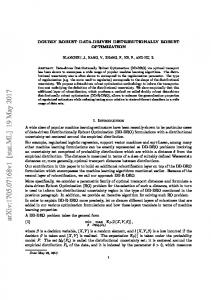
heavily affects the quality of the nominal solution. Flaw of using nominal values. Consider an uncertain linear optimization problem with a single constraint: | a x ≤ b, (1) where a = ¯ a + ρζ is the vector of uncertain coefficients and a ¯ being the nominal vector, ζ ∈ R2 is the uncertain parameter that is uniformly distributed in a unit box ||ζ||∞ ≤ 1, and ρ is a scalar shifting parameter. Now (say) we ignore the uncertainty in the constraint coefficients and solve the associated problem according to the nominal data, i.e., a = ¯ a, and assume that the constraint | is binding for the associated nominal optimal solution x ¯, i.e., ¯ a x ¯ = b. Figure 1 shows the original | constraint [a x ≤ b] in the uncertainty space when x is fixed to the nominal optimal solution x ¯. |
Figure 1: Feasible region of the uncertain constraint (¯ a + ρζ) x ¯ ≤ b in the uncertainty space [−1, 1]2 .
The solid line in Figure 1 represents ζ values where the uncertain constraint is binding when x is fixed to the nominal solution x ¯, and the dashed lines represent the feasible uncertainty region for the same constraint. Therefore, the area that is determined by the intersection of the unit box with the dashed region gives the subset for which the nominal x ¯ is robust. From the figure we can conclude that the probability of violating this constraint can be as high as 50%, since ζ follows a uniform distribution. This shows that uncertainty may severely affect the quality of the nominal solution, and there exists a crucial need for an optimization methodology that yields solutions that are immunized against the uncertainty. Now let us consider the following figure that presents another illustrative example. Figure 2: Effects of uncertainty on feasibility and optimality performance of solutions (this figure is represented in the decision variable space).
In Figure 2, there are three constraints and their binding values are represented by the solid lines. The constraint on the right-hand side is uncertain, and the other two are certain. For the uncertain constraint, the solid line represents the binding value of the constraint for the nominal data and the dashed line represents the same for a different realization of the uncertain data. Notice that, different than in Figure 1, in Figure 2 we are in the space of the decision variable x. We assume that
2
the problem at hand is an uncertain linear problem, therefore, the optimal solutions are obtained at the extreme points of the feasible region where the constraints are binding. Suppose x1 denotes the unique nominal optimal solution of the problem. It is easy to see that x1 may be highly infeasible when the associated constraint is uncertain. The new (robust) optimal solution may become x3 . Now consider the case where x1 and x2 are both optimal for the nominal data, i.e., the optimal facet is the line segment that connects x1 and x2 . In this case, the decision maker would always prefer x2 over x1 , since its feasibility performance is less affected by the uncertainty. This shows that staying away from “risky” solutions that have uncertain binding constraints may be beneficial. There are three complementary approaches in optimization that deals with data uncertainty, namely, robust optimization (RO), stochastic programming (SP), and fuzzy optimization (FO). Each method has its own assumptions, and the way uncertainty is modelled in FO is substantially different than the other two approaches, which shall be explained later in this section. To begin with, as it is pointed out by Ben-Tal et al. (2009, p. xiii), basic SP has the following assumptions: 1) The underlying probability distribution or a family of distributions of the uncertain parameter must be known. 2) The associated distribution or a family of distributions should not change over the time horizon that the decisions are made. 3) The decision maker should be ready to accept probabilistic guarantees as the performance measure against the uncertainty. If these conditions are met and the deterministic counterpart of the stochastic problem is tractable, then SP is the right optimization methodology to solve the problem at hand. For additional details on SP we refer to Pr´ekopa (1995), Birge and Louveaux (2011), Shapiro and Ruszczy´ nski (2003), and Charnes and Cooper (1959). On the other hand, the ‘orthodox’ RO approach has the following three implicit assumptions (Ben-Tal et al. 2009, p. xii): A.1. All decision variables represent “here and now” decisions: they should get specific numerical values as a result of solving the problem before the actual data “reveals itself”. A.2. The decision maker is fully responsible for consequences of the decisions to be made when, and only when, the actual data is within the prespecified uncertainty set. A.3. The constraints of the uncertain problem in question are “hard” – the decision maker cannot tolerate violations of constraints when the data is in the prespecified uncertainty set. It is important to point out that assumption [A.1] can be extended by adjustable robust optimization (ARO); a brief introduction on ARO will be given in Section 3.2. In addition, assumption [A.3] can be relaxed by globalized robust optimization (Ben-Tal et al. 2009, Ch. 3 & 11), as well as by using safe approximations of chance constraints that shall be briefly explained in Section 4. FO is used when data is vague or ambiguous, i.e., unlike RO and SP, the structural properties of the uncertainty such as a probability distribution, the moments of a probability distribution or an uncertainty set, are unknown. More precisely, in FO, one may not be sure with certainty whether an uncertain parameter does or does not belong to a predefined (uncertainty) set since the associated information is ‘fuzzy’ and can only be measured by a membership function. The membership function is generally derived according to non-crisp or subjective judgements of the ‘members’ of the experiment. In the fuzzifying process, subjective judgements of the users are mapped between 0 and 1 by the associated membership function which is often modelled as triangular or trapezoid shaped curves. In fuzzy optimization, the membership functions of fuzzy objective and/or constraints are derived in the fuzzifying step, and then the associated fuzzy mathematical optimization problem is optimized to derive crisp ‘defuzzified’ outputs from the initial non-crisp information at hand. Notice that fuzzifying and defuzzifying steps are conceptually similar to deriving the deterministic counterpart in SP and RO, which shall be explained in Section 3.1 for RO. Nevertheless, instead of using duality and complex mathematical optimization techniques, FO uses simple operators and ‘basic’ OR techniques to optimize membership functions. For further details on FO, we refer reader to Chapter [fill Chapter of the Book on FO]. In the remainder of this section, we compare the three main approaches that are mentioned above: Optimization under uncertainty versus sensitivity analysis. While the objective of RO, SP, and FO is to find the optimal solution that is immunized against the uncertainty of problem 3
data. Sensitivity analysis checks feasibility of the nominal optimal solution for changing values of the nominal data. Therefore, it is misleading to compare sensitivity analysis with optimization under uncertainty approaches since these methods are aimed at completely different questions than sensitivity analysis. Robust optimization versus stochastic programming. If we compare the basic versions of RO and SP, the latter seems to be less conservative than the former since it is not worst-case oriented. However, it is important to point out that the SP approach is valid only when the probability distribution is known. Notice that RO does not have such a restriction since it works with uncertainty sets that can be derived by expert opinion or using historical data. Moreover, the RO paradigm is computationally more tractable than the SP approach; for details on such examples we refer to Ben-Tal et al. (2009, pp. xiii - xv), and Chen et al. (2006). On the other hand, the two approaches may also complement each other under mild assumptions on the uncertainty; see Yanıko˘ glu and Kuhn (2016), and the list of references can be easily extended. Robust optimization & stochastic programming versus fuzzy optimization. RO, SP and FO distinguish from each other by the way they model ambiguity in the uncertainty. We explain similarities and differences among these approaches in threefold: 1) To begin with, SP uses ambiguous chance constraints to model ambiguity in probability distributions; see Section 4. More precisely, different than the classic chance constraint approach, the ambiguity set define a family of probability distributions instead of a unique “known” distribution. Even though an ambiguity set allows the uncertainty to be unknown to some extent, certain probabilistic assumptions are still required for tractability. Nevertheless, ambiguous chance constraints are generally intractable for general classes of probability distributions that are different than Gaussian; for a quick overview, see Nemirovski (2012). Therefore, the SP approach to model ambiguity is impractical when available information at hand is limited and does not follow a specific family of distributions. 2) To model ambiguous uncertain parameters, RO uses the so-called distributionally robust optimization (DRO) framework. Similar to FO, the associated RO methods can be also used when available data is limited. In addition, the associated methods are generally tractable under mild conditions. To model ambiguity sets, DRO uses certain distance measures such as Phi-divergence, Wasserstein metric and etc. to quantify the distance between the nominal data and other realizations defined in the (bounded) ambiguity set; see, Esfahani and Kuhn (2015) and Yanıko˘glu and den Hertog (2013) for applications, and Delage and Ye (2010), Goh and Sim (2010), Wiesemann et al. (2014) for the general theory. 3) Different than RO and SP, FO uses membership functions to model ambiguity in uncertainty. In addition, unlike RO and SP, the way ambiguity is modelled in FO is also subject to vagueness in itself because it is based on vague inputs that do not exhibit any structural properties. On the contrary, SP and RO allow ambiguity to be modelled using certain measures, and the structural properties of the uncertain parameter and the mathematical optimization problem. This is why, the similarities and differences that we have mentioned in this subsection are based on conceptual comparisons.
3
Robust Optimization Paradigm
In this section we first give a brief introduction to RO by presenting the three core steps of deriving the robust counterpart, i.e., the deterministic equivalent of the uncertain optimization problem at hand, which lie at the heart of RO paradigm. Then we present the adjustable robust optimization methodology that enables formulating the wait-and-see decisions, and finalize the section with a procedure for applying RO in practice. For the sake of exposition, we use an uncertain linear optimization problem, but we point out that our discussions in the sequel can be generalized to uncertain nonlinear optimization problems. The “general” formulation of the uncertain linear optimization problem is |
min {c x : Ax ≤ b}(c,A,b)∈U , x
(2)
where c ∈ Rn is a vector of uncertain objective coefficients, A ∈ Rm×n is a matrix of constraint coefficients, and b ∈ Rm denotes an uncertain RHS vector, and U denotes the user specified uncertainty set. As it is explained earlier in Section 2, the RO paradigm is based on the three basic assumptions [A.1], [A.2] and [A.3], namely, x ∈ Rn is a “here and now” decision, true data is assumed to be within the specified uncertainty set U, and constraints are ‘hard’, i.e., constraints violations are not allowed when the data is in U; respectively. In addition to the main “basic”
4
assumptions, we may assume without loss of generality (w.l.o.g.) that: 1) the objective and the right-hand side of the constraint are certain; 2) U is a compact and convex set; and 3) the uncertainty is constraint-wise. Now, we explain why these three assumptions are w.l.o.g. E.1. Suppose the objective coefficients c and the right-hand side vector b are uncertain and (say) they reside in the uncertainty sets C and B; respectively, i.e., the robust reformulation of the uncertain optimization problem is |
min max {c x : Ax ≤ b x
c∈C
∀A ∈ U, ∀b ∈ B}.
Without loss of generality we may assume that the uncertain optimization problem can be equivalently reformulated with a certain objective function and right-hand side: |
min {t : c x − t ≤ 0 x, t
∀c ∈ C, Ax + bxn+1 ≤ 0 ∀(A, b) ∈ U × B},
using an epigraphic reformulation and extra variables t ∈ R and xn+1 = −1. E.2. The uncertainty set U can be replaced by the smallest convex set conv(U), i.e., the convex hull, that includes U because the RC with respect to U is equivalent to taking the supremum of the left-hand side of a constraint over U, which is also equivalent to maximizing the left-hand side over conv(U). For the formal proof, see (Ben-Tal et al. 2009, pp. 12–13). E.3. Robust counterparts of different constraints with respect to the uncertainty set can always be formulated constraint-wise. E.g., consider a problem with two constraints and with uncertain parameters b1 and b2 : x1 +b1 ≤ 0, x2 +b2 ≤ 0, and let U = {b ∈ R2 : b1 ≥ 0, b2 ≥ 0, b1 +b2 ≤ 1} be the uncertainty set. It is easy to see that robustness of the i-th (i=1,2) constraint with respect to U is equivalent to robustness with respect to the projection of U on bi . Ui , i.e., it can be modelled constraint-wise. For the general proof, see (Ben-Tal et al. 2009, pp. 11–12). Notice that the above assumptions are also w.l.o.g. for nonlinear uncertain optimization problems, except the second assumption [E.2].
3.1
Deriving Robust Counterpart
The robust reformulation of (2) that is generally referred to as the robust counterpart (RC) problem is given as follows: | min{c x : A(ζ)x ≤ b ∀ζ ∈ Z , (3) x
L
where ζ ∈ R is the ‘primitive’ uncertain parameter, Z ⊂ Rm×n denotes the user specified uncertainty set, and A(ζ) ∈ Rm×n is the uncertain coefficient matrix and for the sake of simplicity (say) A(ζ) is affine in ζ. A solution x ∈ Rn is called robust feasible if it satisfies the uncertain constraints [A(ζ)x ≤ b] for all realizations of ζ ∈ Z. As it is mentioned above, we may focus on a single constraint because RO can be applied constraint-wise. To this end, a single constraint extracted from (3) can be modeled as follows: |
(a + Pζ) x ≤ b ∀ζ ∈ Z.
(4)
We use a factor model to formulate a single constraint as an affine function a + Pζ of the primitive uncertain parameter ζ ∈ Z, where a ∈ Rn , b ∈ R and P ∈ Rn×L ; for a real-life application of factor models, see Fama and French (1993). Notice that the dimension of the general uncertain parameter Pζ is often much higher than that of the primitive uncertain parameter ζ, i.e., n � L. Notice that (4) contains infinitely many constraints due to the for all (∀) quantifier, i.e., it is a semi-infinite optimization problem that seems intractable in its current form. There are two ways to tackle with such semi-infinite constraints. The first way is to apply robust reformulation techniques to remove the for all quantifier, and the second way is to apply the adversarial approach. In this section, we describe the details of these two approaches. The first approach consists of three steps and the final result will be a computationally tractable RC of (4) that contains a finite number of tractable constraints. Note that this reformulation technique constitutes the core of RO paradigm. We illustrate the three steps of deriving the RC via a polyhedral uncertainty set: Z = {ζ : Dζ + q ≥ 0}, where D ∈ Rm×L , ζ ∈ RL , and q ∈ Rm . 5
Step 1 (Worst-case reformulation). Notice that (4) is equivalent to the following worst-case reformulation: | | | a x + max (P x) ζ ≤ b. (5) ζ: Dζ+q≥0
Step 2 (Duality). We take the dual of the inner maximization problem in (5). The inner maximization problem and its dual yield the same optimal objective value by strong duality. Therefore, (5) is equivalent to | | | | a x + min{q w : D w = −P x, w ≥ 0} ≤ b. (6) w
Step 3 (Robust counterpart). It is important to point out that we can omit the minimization term in (6), since it is sufficient that the constraint holds for at least one w. Hence, the final formulation of the RC becomes | | | | ∃ w : a x + q w ≤ b, D w = −P x, w ≥ 0. (7) Note that the constraints in (7) are linear in x ∈ Rn and w ∈ Rm . |
Table 1: Tractable reformulations for the uncertain constraint [(a + Pζ) x ≤ b ∀ζ ∈ Z] Uncertainty Box Ellipsoidal
Z kζk∞ ≤ 1 kζk2 ≤ 1
Robust Counterpart |
|
a x + kP xk1 ≤ b | | a x + kP xk2 ≤ b
Tractability LP CQP
Table 1 presents the tractable robust counterparts of an uncertain linear optimization problem for box and ellipsoidal uncertainty sets. These robust counterparts are derived using the three steps that are described above. However, we need conic duality instead of LP duality in Step 2 to derive the tractable robust counterparts for the ellipsoidal uncertainty set; see the second row of Table 1. To derive the RC for different classes of uncertainty sets and problem types, one may apply the three steps that are mentioned above by adjusting the second step (‘duality’) of the procedure in order to meet the problem requirements. If the robust counterpart cannot be written as or approximated by a tractable reformulation, we advocate to perform the so-called adversarial approach. The adversarial approach starts with a finite set of scenarios Si ⊂ Zi for the uncertain parameter in constraint i. For example, at the start, Si only contains the nominal scenario. Then, the robust optimization problem, which has a finite number of constraints since Zi has been replaced by Si , is solved. If the resulting solution is robust feasible, we have found the robust optimal solution. If that is not the case, we can find a scenario for the uncertain parameter that makes the last found solution infeasible, e.g., we can search for the scenario that maximizes the infeasibility. We add this scenario to Si , and solve the resulting robust optimization problem, and so on. For a more detailed description, we ¨ refer to Bienstock and Ozbay (2008). It appeared that this simple approach often converges to optimality in a few number of iterations. The advantage of this approach is that solving the robust optimization problem with Si instead of Zi in each iteration, preserves the structure of the original optimization problem. Only constraints of the same type are added, since constraint i should hold for all scenarios in Si . This approach could be faster than reformulating, even for polyhedral uncertainty sets. See Bertsimas et al. (2014) for a comparison. Alternatively, if the probability distribution of the uncertain parameter is known, one may also use the randomized sampling of the uncertainty set proposed by Calafiore and Campi (2005). The randomized approach substitutes the infinitely many robust constraints with a finite set of constraints that are randomly sampled. It is shown that such a randomized approach is an accurate approximation of the original uncertain problem provided that a sufficient number of samples is drawn; see Campi and Garatti (2008, Theorem 1).
3.2
Adjustable Robust Optimization
The first assumption [A.1] of the RO paradigm, i.e., the decisions are here-and-now, can be relaxed by adjustable robust optimization. Namely, in multistage decision making problems, some (or all) decision variables can be modelled as wait-and-see, i.e., one may decide on the value of a waitand-see decision variable after uncertain data reveals itself. For example, the amount of product a factory will manufacture next month may not be a here-and-now decision, but a wait-and-see decision that shall be taken based on the demand of the current month. Therefore, some (or all) decision variables can be adjusted in the time horizon according to a decision rule, which is 6
a function of (some or all part of) the uncertain data. The semi-infinite representation of the adjustable robust counterpart (ARC) is given as follows: |
min {c x : A(ζ)x + By(ζ) ≤ b
∀ζ ∈ Z},
(8)
x,y(·)
where x ∈ Rn is the here-and-now decision that is made before ζ ∈ RL is realized, y(·) ∈ Rk denotes the wait-and-see decision that can be taken when the actual data reveals itself, and B ∈ Rm×k denotes a certain coefficient matrix, i.e., fixed recourse. Nevertheless, the ARC formulation (8) is a complex mathematical optimization problem unless we restrict the function y(ζ) to specific classes such as affine (or linear) decision rules. More precisely, y(ζ) is often approximated by y(ζ) := y0 + Qζ,
(9)
where y0 ∈ Rk and Q ∈ Rk×L are the coefficients in the affine decision rule that are optimized. Affinely adjustable RC (AARC) is famous because it yields tractable reformulations and has many applications in real-life; for more details, see Ben-Tal et al. (2009, Ch. 14) and references therein. Eventually, the tractable reformulation of the constraints in (8): |
{c x : A(ζ)x + By0 + BQζ ≤ d ∀ζ ∈ Z} min 0
x,y ,Q
can be derived by the three step procedure that is described in Section 3.1, since the problem is linear in the uncertain parameter ζ, and the decision variables x, y0 and Q. AARC is equivalent to RC when Q = 0 in (9) and this is why AARC is less conservative than the ‘classic’ RC approach and yields more flexible decisions that can be adjusted according to the realized portion of data at a given stage. Moreover, AARC is a tractable and it does not affect the mathematical optimization complexity of the problem compared with that of the RC, even though, it introduces additional variables. Notice that affine decision rules may also be optimal in some applications areas such as inventory management (Bertsimas et al. 2010) Last but not least, ARO has many applications in real-life, e.g., supply chain management (Ben-Tal et al. 2005), project management (Ben-Tal et al. 2009, Ex. 14.2.1), and engineering (Ben-Tal and Nemirovski 2002a). Remark 1. Tractable ARC reformulations for nonlinear decision rules also exist for specific classes; see Ben-Tal et al. (2009, Ch. 14.3) and Georghiou et al. (2010) for details. Remark 2. A parametric decision rule like (9) cannot be used for integer ‘adjustable’ variables, since we have then to enforce that the decision rule to be integer for all ζ ∈ Z. For alternative methods on modelling adjustable integer variables, we refer to Bertsimas and Caramanis (2007), Vayanos et al. (2011), Bertsimas and Georghiou (2014), Gorissen et al. (2015).
4
Choosing Uncertainty Set
In this section, we describe possible uncertainty sets and their advantages and disadvantages. There is a trade-off between the size (and properties) of the uncertainty set and the optimality performance of the robust optimal solution with respect to this uncertainty set. For example, the box uncertainty set contains the full range of realizations for each individual component of the uncertain parameter. It is the most robust choice because it allows each uncertain component to take its worst-case realization independent from the other components. The box uncertainty set yields tractable RCs with LP complexity for uncertain linear optimization problems, nevertheless, the associated RCs may result in over-conservative objective function values because they yield optimal solutions which are robust against ‘full’ uncertainties where all parameters can take their worst-case realizations at the same time. To overcome the associated over-conservatism, one may use smaller uncertainty sets such as the ellipsoid and the co-axial box, i.e., the intersection of an ellipsoid with a box. Both ellipsoid and co-axial box uncertainty sets introduce some sort of dependence among different components of the uncertainty parameter so that all components cannot take their worst-case realizations at the same time because the total dispersion is bounded by the radius of the ellipsoid. The ellipsoid and co-axial box uncertainty sets are often preferred in practice because they are less conservative than the box and yield tractable RCs that fall in the realm of second-order cone programming (SOCP) given that the original uncertain problem is linear both in terms of the decision variables and the parameters.
7
The practical and theoretical implications behind using the ellipsoid and the co-axial box uncertainty sets are inspired by the chance constraint which is first introduced by Charnes and Cooper (1959). A chance constraint can be represented as: n o | Prζ∼P ζ : a(ζ) x ≤ b ≥ ε, (10) where ζ ∈ RL is the ‘primitive’ uncertain parameter, a ∈ Rn denotes a vector of uncertain coeffin cients, x ∈ R is a vector of decision variables, ε ∈ [0, 1] is the prescribed probability bound, and P is a ‘known’ probability distribution. Different than the classical approach, in the ambiguous chance constraint: n o | Prζ∼P ζ : a(ζ) x ≤ b ≥ ε ∀P ∈ P, (11) P belongs to a family of distributions P. It is important to stress that the ambiguous approach is computationally more challenging than the classical approach because it generalizes one probability distribution to a family of distributions, and is only tractable when the associated family is Gaussian. (Ambiguous) chance constraints are generally intractable because the feasible set is nonconvex, or it is computationally expensive to check the feasibility of constraint, e.g., (10) is bilinear in x and ζ, and ζ follows a uniform distribution. In addition, underlying probability distribution of an uncertain parameter is often unknown or non-existent due to limited data availability or structural properties of the uncertain parameter. To overcome the associated limitations, one way is to use RO to find tractable and (distributionally) safe approximations of the chance constraint. More precisely, we aim to find the uncertainty set Uε such that if x satisfies | a(ζ) x ≤ b ∀ζ ∈ Uε , (12) then x also satisfies (10). Ben-Tal et al. (2009, Chapter 2) show that when Uε is equivalent to the co-axial box uncertainty set: n o L Uεcoax := ζ ∈ R : ||ζ||2 ≤ Ωε , ||ζ||∞ ≤ 1 , (13) a feasible solution for the RC of (12): zj + wj = −[aj ]T x, ∀j ∈ {1, ..., `} v u ` ` X uX w2 ≤ b − [a0 ]T x, |zj | + Ωε t
(14)
j
j=1
j=1
satisfies the chance constraint with at least probability ε, where (z, w) are the additional dual P` variables, a(ζ) = a0 + j=1 ζj aj is affine in the uncertain parameter ζ, Ωε is the radius of the √ ellipsoid that is equivalent to exp(−Ω2 /2) (i.e., Ωε = −2 ln ε), and the uncertain parameter satisfies E[ζi ] = 0, |ζi | ≤ 1 and ζi ’s are independent ∀i ∈ {1, . . . , L}. Another way is to use a polyhedral set (Ben-Tal et al. 2009, Proposition 2.3.4), called budgeted uncertainty set or the Bertsimas and Sim uncertainty set (Bertsimas and Sim 2004): Zε = {ζ : ||ζ||1 ≤ Γ
||ζ||∞ ≤ 1},
(15)
where ε = exp(−Γ2 /(2L)). The probability guarantee of the Bertismas and Sim uncertainty set is only valid when the uncertain parameters are independent and symmetrically distributed. The advantage of the co-axial box is that it is less conservative than the Bertsimas and Sim uncertainty for a fixed ε. Nevertheless, the RC with respect to Bertsimas and Sim uncertainty set is computationally less challenging than the SOCP in (14) because it yields an LP. Bandi and Bertsimas (2012) propose uncertainty sets based on the central limit theorem. When the components of ζ are independent and identically distributed with mean µ and variance σ 2 , the uncertainty set is given by: ) ( L X √ Zε = ζ : | ζi − Lµ| ≤ ρ nσ , i=1
where ρ controls the probability of constraint violation 1 − ε. Bandi and Bertsimas also show variations on Zε that incorporate correlations, heavy tails, or other distributional information. 8
The advantage of this uncertainty set is its tractability, since the robust counterpart of an LP with this uncertainty set is also LP. A disadvantage of this uncertainty set is that it is unbounded for L > 1. Ben-Tal et al. (2013) propose φ-divergence uncertainty sets. The φ-divergence between the vectors p and q is: � � m X pi , Iφ (p, q) = qi φ qi i=1 where φ is the (convex) φ-divergence function; for details on φ-divergence, we refer to Pardo (2005). Let p denote a probability vector and let q be the vector with observed frequencies when N items are sampled according to p. Under certain regularity conditions, 2N d Iφ (p, q) → χ2m−1 as N → ∞. φ00 (1) This motivates the use of the following uncertainty set: Zε = {p : p ≥ 0,
2N ˆ ) ≤ χ2m−1;1−ε }, Iφ (p, p φ00 (1)
|
e p = 1,
ˆ is an estimate of p based on N observations, and χ2m−1;1−ε is the 1 − ε percentile of the χ2 where p distribution with m − 1 degrees of freedom. The uncertainty set contains the true p with (approximate) probability 1 − ε. Ben-Tal et al. (2013) give many examples of φ-divergence functions that lead to tractable robust counterparts. This approach is later extended to general uncertainties in Yanıko˘ glu and den Hertog (2013) to safely approximate ambiguous chances constraints by using historical data. An alternative to φ-divergence is using the Anderson-Darling test to construct the uncertainty set; see, (Ben-Tal et al. 2014, Ex. 15).
5
Miscellaneous Topics
5.1
How to Compare Robust and Nominal Solutions
A common mistake that is often made in practice is to compare the optimal objective function value of a nominal problem with that of its robust reformulation. Notice that a direct comparison is misleading because it is known that both models favour their own objective and it is also know that the robust objective is essentially more conservative than the nominal one. Moreover, we compare objective function values of two different solutions with respect to two different data which are likely to be realized with 0 probability. To fairly compare nominal and robust optimization problems, the best way is to use a Monte Carlo simulation that compares the ‘average’ performance of two mathematical optimization models with respect to a given criteria by sampling uncertain data from a given distribution. The performance criteria can be the average objective function value if the uncertainty is in the objective. If the uncertainty is in the constraints then the performance criteria can be the average number of constraint violations or the average size of the constraint violations. The simulation outcomes can also be analyzed using statistical tests. Gorissen et al. (2015) provide corresponding statistical tests to verify whether one solution is better than the other solution. Suppose the data for a statistics test is available as n pairs (Ri , Ni ) (i = 1, 2, . . . , n), where Ri and Ni are the performance characteristics in the i’th simulation for the robust and the nominal solutions; respectively. Even though it is not necessary for the statistical test that Ri and Ni are based on the same simulated uncertainty vector ζ, it increases the power of the test because Ri and Ni will be positively correlated. It reduces the variance of the difference, i.e., Var(Ri − Ni ) = Var(Ri ) + Var(Ni ) − 2 Cov(Ri , Ni ), which is used in the following statistical tests: • The sign test for the median validates H0 : mR = mN against H1 : mR < mN with confidence level α, where mR and mN are the medians of the distributions of Ri and Ni , respectively. This tests the conjecture that the probability that solution X outperforms solution Y is larger than 0.5. Let n= be the number of observations for which Ri = Ni and let Z be the number of negative signs of Ri − Ni . Under the null hypothesis, Z follows a binomial distribution with parameters n − n= and 0.5. That means that the null hypothesis gets rejected if Z is larger than the (1 − α) percentile of the binomial distribution.
9
• The t-test for the mean validates H0 : µR = µN against H1 : µR < µN with confidence level α, where µx and µy are the means of the distributions of Ri and Ni , respectively. This tests the conjecture that solution R outperforms solution N in long run average behavior. Pn This ¯ test assumes that R − N follows a normal distribution. Let Z = R − N , Z = i i i i i i=1 Zi /n Pn ¯ ¯ 2 /(n − 1), then T = √n Pn (Zi − Z)/s follows a t-distribution with and s2 = i=1 (Zi − Z) i=1 n − 1 degrees of freedom under the null hypothesis. This means that H0 gets rejected if T is smaller than the α percentile of the t-distribution with n − 1 degrees of freedom.
5.2
Robust Counterparts of Equivalent Deterministic Problems are not Necessarily Equivalent
In this section, we show that deterministically equivalent reformulations of a given problem are not necessarily equivalent when we take their robust counterparts. Following examples, taken form Gorissen et al. (2015), provide nice illustrative examples on the associated issue. The first one is similar to the example in Ben-Tal et al. (2009, p. 13). Consider the following constraint: (2 + ζ)x1 ≤ 1, where ζ is an (uncertain) parameter. This constraint is equivalent to: ( (2 + ζ)x1 + s = 1 1 s ≥ 0. However, the robust counterparts of these two constraint formulations, i.e. (2 + ζ)x1 ≤ 1 and
∀ζ : |ζ| ≤ 1,
( (2 + ζ)x1 + s = 1 ∀ζ : |ζ| ≤ 1 s ≥ 0,
(16)
(17)
in which the uncertainty set for ζ is the set {ζ : |ζ| ≤ 1}, are not equivalent. It can easily be verified that the feasible set for robust constraint (16) is: x1 ≤ 1/3, while for the robust constraint (17) this is x1 = 0. The reason why (16) and (17) are not equivalent is that by adding the slack variable, the inequality becomes an equality that has to be satisfied for all values of the uncertain parameter, which is very restrictive. The general message is therefore: do not introduce slack variables in uncertain constraints, unless they are adjustable like in Kuhn et al. (2011), and avoid uncertain equalities. Another example is the following constraint: |x1 − ζ| + |x2 − ζ| ≤ 2, which is equivalent to: y1 + y2 ≤ 2 y1 ≥ x1 − ζ y1 ≥ ζ − x1 y2 ≥ x2 − ζ y ≥ ζ − x . 2 2 However, the robust versions of these two formulations, namely: |x1 − ζ| + |x2 − ζ| ≤ 2 and:
y1 + y2 ≤ 2 y1 ≥ x1 − ζ y1 ≥ ζ − x1 y2 ≥ x2 − ζ y ≥ ζ − x 2 2
∀ζ ∀ζ ∀ζ ∀ζ
∀ ζ : |ζ| ≤ 1,
: : : :
|ζ| ≤ 1 |ζ| ≤ 1 |ζ| ≤ 1 |ζ| ≤ 1,
(18)
(19)
are not equivalent. Indeed, it can easily be checked that the set of feasible solutions for (18) is (θ, −θ), −1 ≤ θ ≤ 1, but the only feasible solution for (19) is x = (0, 0). The reason for this 10
is that in (19) the uncertainty is split over several constraints, and since the concept of RO is constraint-wise, this leads to different problems, and thus different solutions. The following linear optimization reformulation, however, is equivalent to (18): x1 − ζ + x2 − ζ x − ζ + ζ − x 1 2 ζ − x + x − ζ 1 2 ζ − x1 + ζ − x2
≤2 ≤2 ≤2 ≤2
∀ ∀ ∀ ∀
ζ ζ ζ ζ
: : : :
|ζ| ≤ 1 |ζ| ≤ 1 |ζ| ≤ 1 |ζ| ≤ 1.
(20)
For more details on such reformulation issues in different optimization settings, we refer to Gorissen et al. (2015, §6).
5.3
Pareto efficiency
Iancu and Trichakis (2013) discovered that “the inherent focus of RO on optimizing performance only under worst-case outcomes might leave decisions un-optimized in case a non worst-case scenario materialized”. Therefore, the “classical” RO framework might lead to a Pareto inefficient solution; i.e., an alternative robust optimal solution may guarantee an improvement in the objective or slack size for (at least) one scenario without deteriorating it in other scenarios. Given a robust optimal solution, Iancu and Trichakis propose optimizing a new problem to find a solution that is Pareto efficient. In this new problem, the objective is optimized for a scenario in the interior of the uncertainty set, e.g., for the nominal scenario, while the worst-case objective is constrained to be not worse than the robust optimal objective value. For more details on Pareto efficiency in robust linear optimization we refer to Iancu and Trichakis (2013).
6
Conclusion
In this chapter, we have presented the core methodologies to successfully apply RO paradigm. In addition, we have also presented advantages and disadvantages of the associated methods as well as limitations and common wrong doings while applying the RO procedure. Presented topics are based on current advances of RO and for new comers they are good outlet for applying RO in practice. Future research directions on RO could be on ARO, as it is explained before, more research is needed on adjustable integer variables and applications of ARO for MIP problems. To point out, efficient local search algorithms to solve MIP formulations are generally not viable in RO because at each stage the worst-case realization has to be found and this may be costly. This is why efficient solution methodologies tailored for RO to solve challenging uncertain MIP formulations are also required. Last but not least, applications or RO (and specifically ARO) are still lagging behind, especially. more research on semi-conductor manufacturing, engineering design optimization, and humanitarian logistics are scarce, and more research on these topics is needed.
Acknowledgement This work is supported by Scientific and Technological Research Council of Turkey (TUBITAK) through BIDEB 2232 Research Grant (115C100) of the author.
References F. Babonneau, J.-P. Vial, and R. Apparigliato. Robust optimization for environmental and energy planning. In Uncertainty and Environmental Decision Making, pages 79–126. Springer, 2010. URL http: //dx.doi.org/10.1007/978-1-4419-1129-2_3. C. Bandi and D. Bertsimas. Tractable stochastic analysis in high dimensions via robust optimization. Mathematical Programming, 134(1):23–70, 2012. URL http://dx.doi.org/10.1007/s10107-012-0567-2. A. Ben-Tal and A. Nemirovski. Robust solutions of linear programming problems contaminated with uncertain data. Mathematical Programming, 88(3):411–424, 2000. A. Ben-Tal and A. Nemirovski. Robust optimization–methodology and applications. Mathematical Programming, 92(3):453–480, 2002a. URL http://dx.doi.org/10.1007/s101070100286. A. Ben-Tal and A. Nemirovski. Robust optimization – methodology and applications. Mathematical Programming, 92(3):453–480, 2002b.
11
A. Ben-Tal, B. Golany, A. Nemirovski, and J.-P. Vial. Retailer-supplier flexible commitments contracts: A robust optimization approach. Manufacturing & Service Operations Management, 7(3):248–271, 2005. URL http://dx.doi.org/10.1287/msom.1050.0081. A. Ben-Tal, L. El Ghaoui, and A. Nemirovski. Robust Optimization. Princeton Series in Applied Mathematics. Princeton University Press, 2009. URL http://sites.google.com/site/robustoptimization/. A. Ben-Tal, D. den Hertog, A. M. B. De Waegenaere, B. Melenberg, and G. R. Rennen. Robust solutions of optimization problems affected by uncertain probabilities. Management Science, 59(2):341–357, 2013. A. Ben-Tal, D. den Hertog, and J.-P. Vial. Deriving robust counterparts of nonlinear uncertain inequalities. Mathematical Programming, Online First, 2014. URL http://dx.doi.org/10.1007/ s10107-014-0750-8. D. Bertsimas and C. Caramanis. Adaptability via sampling. In 46th IEEE Conference on Decision and Control, pages 4717–4722, 2007. D. Bertsimas and A. Georghiou. Binary decision rules for multistage adaptive mixed-integer optimization. Mathematical Programming, pages 1–39, 2014. D. Bertsimas and M. Sim. The price of robustness. Operations Research, 52(1):35–53, 2004. URL http: //dx.doi.org/10.1287/opre.1030.0065. D. Bertsimas and A. Thiele. A robust optimization approach to inventory theory. Operations Research, 54(1):150–168, 2006. D. Bertsimas, D. A. Iancu, and P. A. Parrilo. Optimality of affine policies in multistage robust optimization. Mathematics of Operations Research, 35(2):363–394, 2010. URL http://dx.doi.org/10.1287/moor. 1100.0444. D. Bertsimas, D. Brown, and C. Caramanis. Theory and applications of robust optimization. SIAM Review, 53(3):464–501, 2011. D. Bertsimas, E. Litvinov, X. A. Sun, J. Zhao, and T. Zheng. Adaptive robust optimization for the security constrained unit commitment problem. IEEE Transactions on Power Systems, 28(1):52–63, 2013. URL http://dx.doi.org/10.1109/TPWRS.2012.2205021. D. Bertsimas, I. Dunning, and M. Lubin. Reformulations versus cutting planes for robust optimization: A computational and machine learning perspective. Optimization Online, April, 2014. URL http: //www.optimization-online.org/DB_HTML/2014/04/4336.html. H.-G. Beyer and B. Sendhoff. Robust optimization – a comprehensive survey. Computer Methods in Applied Mechanics and Engineering, 196(33–34):3190–3218, 2007. ¨ D. Bienstock and N. Ozbay. Computing robust basestock levels. Discrete Optimization, 5(2):389–414, 2008. J. R. Birge and F. V. Louveaux. Introduction to Stochastic Programming. Springer, 2011. G. Calafiore and M. C. Campi. Uncertain convex programs: randomized solutions and confidence levels. Mathematical Programming, 102(1):25–46, 2005. URL http://dx.doi.org/10.1007/ s10107-003-0499-y. M. C. Campi and S. Garatti. The exact feasibility of randomized solutions of uncertain convex programs. SIAM Journal on Optimization, 19(3):1211–1230, 2008. A. Charnes and W. W. Cooper. Chance-constrained programming. Management Science, 6(1):73–79, 1959. X. Chen, M. Sim, P. Sun, and J. Zhang. A tractable approximation of stochastic programming via robust optimization. Operations Research, 2006. E. Delage and Y. Ye. Distributionally robust optimization under moment uncertainty with application to data-driven problems. Operations research, 58(3):595–612, 2010. P. M. Esfahani and D. Kuhn. Data-driven distributionally robust optimization using the wasserstein metric: Performance guarantees and tractable reformulations. arXiv preprint arXiv:1505.05116, 2015. E. F. Fama and K. R. French. Common risk factors in the returns on stocks and bonds. Journal of Financial Economics, 33(1):3–56, 1993. A. Fredriksson, A. Forsgren, and B. H˚ ardemark. Minimax optimization for handling range and setup uncertainties in proton therapy. Medical Physics, 38(3):1672–1684, 2011. URL http://dx.doi.org/. V. Gabrel, C. Murat, and A. Thiele. Recent advances in robust optimization: An overview. European journal of operational research, 235(3):471–483, 2014. A. Georghiou, W. Wiesemann, and D. Kuhn. Generalized decision rule approximations for stochastic programming via liftings. Optimization Online, 2010. J. Goh and M. Sim. Distributionally robust optimization and its tractable approximations. Operations research, 58(4-part-1):902–917, 2010. ˙ Yanıko˘ B. L. Gorissen, I. glu, and D. den Hertog. A practical guide to robust optimization. Omega, 53: 124–137, 2015.
12
D. Iancu and N. Trichakis. Pareto efficiency in robust optimization. Management Science, online first, 2013. D. Kuhn, W. Wiesemann, and A. Georghiou. Primal and dual linear decision rules in stochastic and robust optimization. Mathematical Programming, 130(1):177–209, 2011. S. Lim. A joint optimal pricing and order quantity model under parameter uncertainty and its practical implementation. Omega, 41(6):998–1007, 2013. URL http://dx.doi.org/10.1016/j.omega.2012. 12.003. M. S. Lobo. Robust and convex optimization with applications in finance. PhD thesis, Stanford University, 2000. URL http://sousalobo.com/thesis/thesis.pdf. A. Nemirovski. On safe tractable approximations of chance constraints. European Journal of Operational Research, 219(3):707–718, 2012. L. Pardo. Statistical inference based on divergence measures. CRC press, 2005. A. Pr´ekopa. Stochastic Programming. Kluwer Academic Publishers, 1995. A. Shapiro and A. P. Ruszczy´ nski. Stochastic Programming. Elsevier, 2003. P. Vayanos, D. Kuhn, and B. Rustem. Decision rules for information discovery in multi-stage stochastic programming. In Decision and Control and European Control Conference (CDC-ECC), 2011 50th IEEE Conference on, pages 7368–7373. IEEE, 2011. X. Wang and D. J. Curry. A robust approach to the share-of-choice product design problem. Omega, 40 (6):818–826, 2012. W. Wiesemann, D. Kuhn, and M. Sim. Distributionally robust convex optimization. Operations Research, 62(6):1358–1376, 2014. S. Yan and C.-H. Tang. Inter-city bus scheduling under variable market share and uncertain market demands. Omega, 37(1):178–192, 2009. ˙ Yanıko˘ I. glu and D. den Hertog. Safe approximations of ambiguous chance constraints using historical data. INFORMS Journal on Computing, 25(4):666–681, 2013. ˙ Yanıko˘ I. glu and D. Kuhn. Decision rule bounds for stochastic bilevel programs. Technical report, 2016.
13