[29] M. Cummins, P. Newman, FAB-MAP: Probabilistic localization and mapping in the space of ap- pearance. The International Journal of Robotics Research, ...
Robust Place Recognition Based on Omnidirectional Vision and Real-time Local Visual Features for Mobile Robots Huimin Lu, Xun Li, Hui Zhang, and Zhiqiang Zheng College of Mechatronics and Automation, National University of Defense Technology, Changsha, China, {lhmnew, lixun, huizhang nudt, zqzheng}@nudt.edu.cn
Abstract Topological localization is especially suitable for human-robot interaction and robot’s high level planning, and it can be realized by visual place recognition. In this paper, bag-of-features, a popular and successful approach in pattern recognition community, is introduced to realize robot topological localization. By combining the real-time local visual features proposed by ourselves for omnidirectional vision and support vector machines, a robust and real-time visual place recognition algorithm based on omnidirectional vision is proposed. The panoramic images from the COLD database were used to perform experiments to determine the best algorithm parameters and the best training condition. The experimental results show that the robot can achieve robust topological localization with high successful rate in real-time by using our algorithm.
keywords: Place recognition, Omnidirectional vision, Local visual features, Robot topological localization
1
INTRODUCTION
According to the different ways to represent navigation maps for mobile robots, robot localization can be divided into metric, topological and hybrid localization [1]. In metric localization [2], mobile robots should obtain localization coordinates as accurately as possible. In topological localization [3], only the abstract localization should be provided, like “the robot is in the kitchen”, “the robot is in the corridor”, etc. In hybrid localization [4], hierarchical maps are built to realize both topological localization and metric localization. In the complex unstructured environments, it is usually difficult to recognize and measure natural landmarks by vision sensors, so accurate visual metric localization is hard to realize, and topological localization becomes a more feasible choice. Furthermore, topological localization is especially suitable for human-robot interaction and robot’s high level planning [5]. For example, human only need to “tell” robots to go to some place instead of giving an accurate coordinate. Visual topological localization has become a research focus in computer/robot vision community. In recent years, along with the development of image understanding and pattern recognition, visual place/scene recognition has attracted more and more researchers’ interest, and many progresses have 1
been achieved [1, 6, 7, 8, 9], which makes it possible to realize topological localization based on place recognition. If the nodes of topological maps are represented by the places like kitchen, corridor, and bathroom, once these places are recognized and classified by robots, topological localization is also realized for the robots. Besides topological localization, place recognition is also important for solving the loop closing in visual odometry [10], visual SLAM [11] and the kidnapping problem in robot localization [12]. On the research of topological localization based on place recognition, lots of new approaches can be referred from computer vision and pattern recognition community, which will also promote the fusion of the research in computer vision, pattern recognition, and robotics communities. In this paper, bag-of-features [13, 14], a popular and successful approach in pattern recognition community, is introduced to realize robust topological localization for mobile robots by combining two novel real-time local visual features for omnidirectional vision [15] and support vector machines (SVMs) [16]. In the following parts, related research will be discussed in Section 2, and bag-of-features and SVMs will be introduced briefly in Section 3. In Section 4, two real-time local visual features for omnidirectional vision, namely FAST+LBP and FAST+CSLBP, will be presented. Then we will propose our robust and real-time place recognition algorithm based on omnidirectional vision for robot topological localization in Section 5. The thorough experiments will be performed by using the COLD database [17] to determine the best algorithm parameters and the best training condition, and to validate the effectiveness of our algorithm in Section 6. The conclusion will be given in Section 7 finally.
2
RELATED RESEARCH
In the complex and unstructured environment, it is difficult to recognize natural landmarks directly, so the visual appearance based matching approaches are commonly used in robot topological localization, which is similar with the mechanism of image retrieval. The visual appearance consists of global visual features and local visual features. In comparison with the localization approaches using global visual features like color histograms [18], gradient orientation histograms [19], edge density histograms [19], etc., better performance can be achieved by the localization approaches using local visual features like SIFT [20, 21], iterative SIFT [22], SURF [4], etc., because local visual features have better discriminative power, and are more robust with respect to occlusion, image translation, changes of view. Meanwhile, the computation costs of the approaches using local visual features are usually much higher than that of those methods using global visual features, because much more time should be used to extract local visual features from images. Some researchers also found that robustness and efficiency of the robot localization system can be improved by integrating both global and local visual features together in their algorithms [23, 24]. In these localization methods, whether using global or local visual features, the corresponding visual appearances should be stored in the memory off-line for each node of the topological map to build up a map database. During the on-line topological localization process, the visual appearances of the image acquired currently by the robot are extracted, and then they are used to match with the stored appearances in the map database, so the node where the robot locates can 2
be retrieved. When the environment is large-scale, large memory space is needed and the computation cost for feature matching is also high. Furthermore, the used visual appearance, whether global or local visual features, is hard to understand directly for human. These localization methods are inconsistent with the way human recognize the environment and realize localization. So extracting the high level semantic information human can understand like place, scene, etc. from images becomes a better choice to realize visual topological localization. Pronobis, Caputo, Luo, et al. proposed a robust place recognition algorithm based on SVMs classifier, combined with local visual features computed using a Harris-Laplace detector and the SIFT descriptor in [25]. Because the number of the local visual features in an image is not fixed, the local descriptors are used as the input of SVMs via a matching kernel [26]. Then the classifiers can be trained for place classification and recognition. The local visual features are used as the input of SVMs directly, so large memory space is needed to store those features used as support vectors. Therefore, they proposed a memory-controlled incremental SVMs by combining an incremental extension of SVMs with a method reducing the number of support vectors needed to build the decision function without any loss in performance introducing a parameter which permits a user-set trade-off between performance and memory in [9]. They also built up several image databases to provide standard benchmark datasets for the development, evaluation and comparison of different topological localization algorithms: the INDECS [1], the IDOL [1] and the COLD [17] database. All the images in these databases were acquired in indoor environments and with different conditions like different robot platforms, different lighting conditions, and different labs across Europe. Although the COLD database includes panoramic images acquired by the omnidirectional vision system, only perspective images were used to perform experiments to test their place recognition methods in [9, 25]. Some researchers used or extended the bag-of-features method to realize qualitative localization [27], global localization [28], or topological SLAM [29], which are the most similar research with our work in this paper. Only perspective images were used in their work. Furthermore, the local visual features used in their work can not be extracted in real-time, so their algorithms can not be run in real-time actually.
3 3.1
BAG-OF-FEATURES AND SVMs Bag-of-features
Bag-of-features [13, 14] is motivated by learning methods using the bag-of-words representation for text categorization. The text is represented by a vector with components given by the occurrence frequency of the words in the vocabulary, and then it can be categorized by using the vector as the input of the Bayes or SVMs classifier. In recent years, this idea has been adapted to be bag-of-features in computer vision/pattern recognition community. Bag-of-features has become a popular approach, and has been applied successfully to object recognition [30], video retrieval [31], scene classification [32, 33], etc.
3
Bag-of-features is divided into learning/training phase and recognition/testing phase. In the training phase, local visual features are extracted from all the training images, and then these features are clustered by using K-means clustering or other algorithms. The clustering centers can form a visual vocabulary, and every feature from the training images can also be assigned to the nearest cluster. Each training image can be represented by a normalized vector with components given by the occurrence frequency of each feature in the visual vocabulary. These vectors and the corresponding categories are used to train the classifiers. In the testing phase, the testing image is also represented by a normalized vector computed in the same way, and then the vector is used as the input of the trained classifier to realize recognition/classification.
3.2
Support vector machines
SVMs [16] is one of the most popular and successful classifier learning methods in pattern recognition. It has solid mathematic foundation, and its main idea is to find a hyperplane which separates two-class data with maximal margin. The margin is defined as the distance of the closest training point to the separating hyperplane. When data sets are not linearly separable, SVMs takes a mapping from the original data space to another feature space with higher or even infinite dimension to make the data linearly separable in the second feature space. So a nonlinear SVMs can be constructed by replacing the inner product in the linear SVMs with a kernel function. Kernels commonly used include linear kernel, RBF kernel, Sigmoid kernel, etc. In order to apply SVMs to multi-class problems, one-vs-one or one-vs-all strategy can be used. Given an m-class problem, m(m − 1)/2 SVMs classifiers should be trained in the former strategy, and each classifier distinguishes every two categories. In the latter strategy, only m classifiers should be trained, and each classifier distinguishes one category from the rest categories.
4
TWO REAL-TIME LOCAL VISUAL FEATURES FOR OMNIDIRECTIONAL VISION
Although local visual features have been applied successfully in many computer/robot vision problems [34], a common deficiency for most of the current local visual features is that their computation costs are usually high. This deficiency limits the application of local visual features in those situations with high real-time requirements like robot navigation, self-localization. So we proposed two novel real-time local visual features for omnidirectional vision [15]. Features from Accelerated Segment Test (FAST) [35] is used as the feature detector, and local binary pattern (LBP) [36] and center-symmetric local binary pattern (CS-LBP) [36] as feature descriptors, so two algorithms named FAST+LBP and FAST+CSLBP were designed. FAST, LBP and CS-LBP are computationally simple, so they can be the basis of our real-time local visual features. The algorithms are divided into three steps:
4
(a)
(b)
(c)
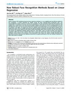
Figure 1: The final FAST+LBP algorithm. (a) A feature region on the panoramic image. The green points are the detected corner features. (b) The scale-up feature region. The region is divided into 2×2 cells. (c) The resulting feature descriptor. The descriptor dimension is 236. - FAST feature detector: According to the experiments in [35], among the several FAST algorithms, FAST 9 seems to be the best one, and it is over five times faster than the quickest non-FAST detector. The FAST algorithm also significantly outperforms Harris, DoG, Harris-Laplace, SUSAN, etc. in repeatability. So FAST 9 was chosen as the feature detector for our real-time local visual features to detect corner features in the panoramic image. - Feature region determination: After a corner feature has been detected, a surrounding image region should be determined, and then a descriptor can be extracted from the image region. We adopted the feature region determining method proposed in [37] to achieve rotation invariance. Rectangular image regions surrounding corner features are firstly determined in the radial direction, and then rotated to a fixed orientation, as shown in Fig. 1(a) and Fig. 2(a). During the rotation process, bilinear interpolation is used. - Feature descriptor with LBP and CS-LBP: The final step of the local visual feature algorithm is to describe the features by computing vectors according to the information of feature regions. An LBP or CS-LBP value for each pixel of the feature region can be computed according to the introduction in [36]. In order to incorporate spatial information into the descriptor, the feature region can be divided into different grids such as 1×1 (1 cell), 2×2 (4 cells), 3×3 (9 cells), and 4×4 (16 cells). For each cell, the histogram of LBP or CS-LBP values is created, and then all the histograms are concatenated into a vector as the descriptor. Finally, the descriptor is normalized to unit length. The descriptor dimension is M ×M ×the histogram dimension for M ×M cells. In computing the histogram, the LBP or CS-LBP values can be weighted with a Gaussian window overlaid over the whole feature region, or with uniform weights over the whole region. The latter means that the feature weighting is omitted. We performed feature matching experiments by using the panoramic images in the COLD database [17] to determine the best algorithm parameters and to compare with SIFT [38]. The final FAST+LBP and FAST+CSLBP with best algorithm parameters are shown in Fig. 1 and Fig. 2 respectively. The descriptor dimension of FAST+LBP and FAST+CSLBP are 236 and 72. The experimental results in [15]
5
(a)
(b)
(c)
Figure 2: The final FAST+CSLBP algorithm. (a) A feature region on the panoramic image. The green points are the detected corner features. (b) The scale-up feature region. The region is divided into 3×3 cells. (c) The resulting feature descriptor. The descriptor dimension is 72. show that our algorithms have better performance than SIFT. The computation time needed to extract all the features in an image by FAST+LBP or FAST+CSLBP is from 5ms to 20ms, so our local visual features can be extracted in real-time, and they can be applied to computer/robot vision tasks with high real-time requirements like place recognition in this paper. Their performance will be compared with SIFT and SURF [39] when applied to place recognition in Section 6.2.
5
ROBUST PLACE RECOGNITION ALGORITHM BASED ON OMNIDIRECTIONAL VISION
In this section, we introduce bag-of-features into robotics community, and try to achieve robust and real-time place recognition for robot topological localization by combining the real-time local visual features for omnidirectional vision presented in Section 4 and SVMs. Our place recognition algorithm is divided into two phases: the phase of off-line training and the phase of on-line testing. The diagram of the algorithm is demonstrated in Fig. 3. In the phase of off-line training, we assume that the number of the panoramic images for training is m, the number of place categories is M , and the corresponding place category of each image is also ∑m known. The local visual features fi are extracted from each training image, where i = 1... j=1 nj , and nj is the number of the local visual features extracted from the jth training image. After clustering these features with K-means clustering algorithm, we get clustering centers Ci , where i = 1...k, and k is the clustering number. These clustering centers compose the visual vocabulary which is similar as the word vocabulary for text categorization. After the clustering is finished, each local visual feature from the training image has also been assigned to the corresponding cluster, which means that the feature type is obtained. A feature vector xj is computed by normalizing the histogram constructed with the number of occurrences of each type
6
Figure 3: The diagram of our place recognition algorithm based on omnidirectional vision and local visual features.
7
of the features from the visual vocabulary in the jth training image, where xj ∈Rk . The feature vector is an effective representation of the image information, and it is named as bag of features. Then the bags of features and the corresponding place categories of all training images are used to learn M classifiers by applying the famous SVMs software - LIBSVM [40] according to the one-vs-all strategy. During the training process mentioned above, the algorithm setup like the different local visual features, the different clustering numbers, the different kernel functions, and the completeness of the visual vocabulary, will affect the performance of our place recognition algorithm. We will determine the best algorithm setup by experiments in the next section. In the phase of on-line testing, the local visual features are extracted from the testing panoramic image (or the image acquired on-line by the robot’s vision system), and then each local visual feature is assigned to a feature type according to its distances to the clustering centers by the nearest neighboring principle. The bag of features of the testing image is computed by normalizing the histogram constructed with the number of occurrences of each type of the features from the visual vocabulary in the testing image. Finally, this bag of features is used as the input of the learned M classifiers, and the outputs are the classification results and the corresponding classification probability. The classification result with the largest classification probability is used as the final place category. When the nodes of the robot’s navigation map are represented with place categories, finishing place recognition means that the topological localization in the navigation map is also realized. In comparison with the topological localization methods based on feature matching directly, we extract the place information in the semantic level from panoramic images to realize topological localization, so our method is more consistent with the way human recognize the environment and realize localization. Omnidirectional vision is used in our method, and better performance in place recognition should be achieved than those methods only using perspective images, because omnidirectional vision can provide a 360o view of the robot’s surrounding environment in a single image, which will be verified by the experimental results in the next section.
6
THE EXPERIMENTAL RESULTS
In this section, a series of experiments will be performed to test our place recognition algorithm. Firstly, we will introduce the experimental setup briefly. Then we will test and analyze that how the algorithm performance will be affected by the factors like the choice of the local visual feature, the clustering number, the kernel function, the training condition, and the occlusion of omnidirectional vision. Therefore, the best algorithm parameters and the best training condition can be determined. The performance will be presented in detail when the best parameters and the best training condition are used. The comparison of the performance will also be performed with the most famous algorithm proposed in [9, 25]. Finally the real-time performance and the needed memory will be discussed. In the paper, the place classification rate equals to the successful rate of robot topological localization.
8
Figure 4: The typical panoramic images acquired in different places and under different illumination conditions. The places are as follows from left to right: corridor, one-person office, printer area, and bath room. The illumination conditions are as follows from top to bottom: cloudy, sunny, and night.
6.1
Experimental setup
COLD is a freely available database which provides a large-scale, flexible testing environment for visionbased topological localization. COLD contains 76 image sequences acquired in three different indoor environments across Europe. The images are acquired by the same perspective and omnidirectional vision in different rooms and under various illumination conditions. We will use the following six sequences of the panoramic images in COLD-Saarbruecken to perform our experiments: seq3 cloudy1, seq3 cloudy2, seq3 night1, seq3 night2, seq3 sunny1, seq3 sunny2. The “cloudy”, “night”, and “sunny” indicate the corresponding illumination conditions under which the image sequences are acquired. Four places are included in each of these image sequences: corridor, one-person office, printer area, and bath room. Some typical panoramic images are shown in Fig. 4. Although there are only four places, the sequences are long-term, and over 700 panoramic images are included in each sequence. More details about COLD can be found in [17]. In the following experiments, we will use some image sequence to train the SVMs classifiers, and some other sequences to test and evaluate the algorithm performance.
9
6.2
The choice of the local visual feature
In this experiment, we compare the algorithm performance when using different local visual features: FAST+LBP, FAST+CSLBP, SIFT [38], and SURF [39]. The clustering number was set to be 200, and linear kernel was used in SVMs. During the experiment, we used the image sequence seq3 cloudy1, seq3 night2, seq3 sunny2 for training respectively, and then used seq3 cloudy2, seq3 night1, seq3 sunny1 for testing respectively. Because there is a certain degree of randomness in the clustering results obtained by using K-means clustering algorithm, the training and testing processes were run several times to get the average place classification rate. The experimental results are shown in Table 1 when different local visual feature was chosen. We see that the overall performance is much better when using FAST+LBP or FAST+CSLBP than using SIFT or SURF. There is not much difference in the overall performance when using FAST+LBP or FAST+CSLBP. However, the descriptor dimension of FAST+CSLBP is 72, and it is much smaller than that of FAST+LBP, which causes the lower computation cost of the place recognition algorithm. So we choose FAST+CSLBP as the local visual feature in the following experiments. Table 1: The place classification rates when choosing different local visual feature in the algorithm. training seq3 cloudy1
seq3 night2
seq3 sunny2
FAST+LBP
0.9375
0.9245
0.8216
seq3 cloudy2
FAST+CSLBP
0.9611
0.9364
0.9468
for testing
SIFT
0.8168
0.7282
0.8361
SURF
0.8313
0.7255
0.7954
FAST+LBP
0.9472
0.9621
0.9149
seq3 night1
FAST+CSLBP
0.9254
0.8659
0.9470
for testing
SIFT
0.8495
0.8342
0.8892
SURF
0.7225
0.7849
0.8150
FAST+LBP
0.8867
0.7238
0.7493
seq3 sunny1
FAST+CSLBP
0.8666
0.6802
0.6863
for testing
SIFT
0.8083
0.7362
0.6335
SURF
0.7760
0.7711
0.7813
According to Table 1, the classification rates with SURF are higher than that with FAST+CSLBP when using seq3 night2 or seq3 sunny2 for training, and seq3 sunny1 for testing. To analyze it, we compared the numbers of the local visual features extracted from the six image sequences by using FAST+CSLBP and SURF, as shown in Fig. 5, from which we see that the fluctuation of the numbers by using FAST+CSLBP is higher than that by using SURF. This is because FAST detector is sensitive to lighting conditions. We also chose one typical image from each sequence when the robot is located in the same position where the acquired images are affected greatly by the lighting conditions, as shown 10
The number of features extracted from different image sequences by using FAST+CSLBP 450
Number of Local Visual Features
350 300
Number of Local Visual Features
seq3__cloudy1 seq3__cloudy2 seq3__night1 seq3__night2 seq3__sunny1 seq3__sunny2
400
250 200 150 100
The number of features extracted from different image sequences by using SURF 300 seq3__cloudy1 seq3__cloudy2 seq3__night1 250 seq3__night2 seq3__sunny1 seq3__sunny2 200
150
100
50 50 0
0
100
200
300
400 500 Image Number
600
700
800
0
900
(a)
0
100
200
300
400 500 Image Number
600
700
800
900
(b)
Figure 5: The numbers of the local visual features extracted from the six image sequences by using FAST+CSLBP (a) and SURF (b). The dashed lines represent the average numbers of the features extracted from each image sequence. in Fig. 6, and then extracted the features by using FAST+LBP and SURF, and performed feature matching. The results are shown in Table 2, which also validate that the extraction and matching of SURF features are more stable than that of FAST+CSLBP under different lighting conditions. So the place classification rates with SURF are also more stable than that with FAST+CSLBP, as shown in Table 1. When using different sequences with quite different numbers of features for training and testing, the place classification rate with FAST+CSLBP may decrease because of the possible incompleteness of the visual vocabulary, as explained in Section 6.5, so the place classification rates with SURF may be higher than that with FAST+CSLBP under these training and testing conditions. However, because the discriminative power of FAST+CSLBP is good [15], which can also be validated by the ratio between the number of correct matches and the number of matches in Table 2, the overall performance with FAST+CSLBP is better than that with SURF.
6.3
The clustering number
In this experiment, we compare the algorithm performance affected by different clustering numbers. FAST+CSLBP and linear kernel were used in the algorithm. During the experiment, we used the image sequence seq3 cloudy1 for training, and then used seq3 cloudy2, seq3 night1, seq3 sunny1 for testing respectively. The training and testing processes were also performed several times to get the average place classification rate. The experimental results are shown in Fig. 7 when the clustering number was set to be 50, 100, 150, 200, 250, 300, 350 and 400. From Fig. 7, we see that sometimes the classification rate is not affected greatly by the clustering number, and especially when using seq3 cloudy2 for testing, all the classification rates are high when setting different clustering numbers. However, in the general trend, the algorithm performance increases as the increase of the clustering number, which is consistent with the research results [13, 33] in pattern recognition community. But the increase of the clustering
11
(a)
(b)
(c)
(d)
(e)
(f)
Figure 6: The typical panoramic images chosen from each image sequences. (a) and (d) are from seq3 cloudy1 and seq3 cloudy2, (b) and (e) are from seq3 night1 and seq3 night2, and (c) and (f) are from seq3 sunny1 and seq3 sunny2. number will make the vocabulary size larger and then cause higher computation cost in the testing process, so a compromise should be made between the classification rate and the clustering number. In the following experiments, the clustering number will be set to be 300 as the best parameter.
6.4
The choice of the kernel function in SVMs
In this experiment, we compare the algorithm performance affected by using different kernel functions in SVMs: linear kernel, RBF kernel, Sigmoid kernel. FAST+CSLBP was used, and the clustering number was set to be 300 in the algorithm. During the experiment, we used the image sequence seq3 cloudy1 for training, and then used seq3 cloudy2, seq3 night1, seq3 sunny1 for testing respectively. The training and testing processes were also performed several times to get the average place classification rate. The experimental results are shown in Table 3. We see that there is not much difference in the overall performance when using different kernel functions. Because linear kernel is computationally simplest, it will be used as the best kernel function in the following experiments.
6.5
The completeness of the visual vocabulary
In this experiment, the best algorithm parameters determined above were used, which means that FAST+CSLBP and linear kernel were chosen, and the clustering number was set to be 300. During the experiment, we used the image sequence seq3 cloudy1, seq3 night2, seq3 sunny2 for training respectively, and then used seq3 cloudy2, seq3 night1, seq3 sunny1 for testing respectively. The average place
12
Table 2: The results of feature extraction and feature matching when using FAST+CSLBP and SURF. The results before and behind “/” correspond to FAST+CSLBP and SURF respectively.
Image
Fig. 6(a)
Fig. 6(d)
Fig. 6(e)
Number of features
180/205
179/216
81/148
Fig. 6(d) 179/216
Fig. 6(f)
Fig. 6(d)
163/178
179/216
Number of matches
123/154
40/122
89/138
Number of correct matches
107/114
27/72
73/87
Image Number of features
Fig. 6(a) 180/205
Fig. 6(b) 90/163
Fig. 6(e) 81/148
Fig. 6(b) 90/163
Fig. 6(f) 163/178
Fig. 6(b) 90/163
Number of matches
40/147
68/138
56/135
Number of correct matches
28/34
66/122
20/42
Image
Fig. 6(a)
Fig. 6(c)
Fig. 6(e)
Number of features
180/205
189/214
81/148
Fig. 6(c) 189/214
Fig. 6(f)
Fig. 6(c)
163/178
189/214
Number of matches
111/154
47/113
115/152
Number of correct matches
99/108
36/39
108/112
Table 3: The place classification rates when different kernel functions were used in the algorithm. linear kernel
RBF kernel
Sigmoid kernel
seq3 cloudy2 for testing
0.9521
0.9632
0.9313
seq3 night1 for testing
0.9594
0.9477
0.9516
seq3 sunny1 for testing
0.9336
0.9475
0.9476
classification rates were acquired to compare which image sequence was best for training to achieve the best performance. The experimental results are shown in Table 4. As shown in Fig. 5(a), the order of the illumination condition is “sunny”, “cloudy” and then “night” from large to small according to the number of features extracted from the corresponding image sequences by using FAST+CSLBP. When using one sequence with small number of features for training and another sequence with large number of features for testing, the visual vocabulary may be incomplete, and the incompleteness of the visual vocabulary will lead to the decrease of the place classification rate, which is the same as the situation in text categorization that the incompleteness of the word vocabulary will result in the decrease of the text categorization rate. So in this regard, the image sequence acquired under “sunny” illumination condition should be best for training. However, because the “sunny” illumination is most unstable, and FAST+CSLBP is sensitive to the illumination condition, the place classification rate may be low when using another “sunny” sequence for testing, as shown in Table 4. The “cloudy” illumination is more stable than “night” and “sunny”, and all the classification rates are high when using the image sequence acquired under “cloudy” illumination condition for training in Table 4. The same conclusion can also be obtained from the experimental results in Section 6.2. So we consider the image sequence acquired under “cloudy” illumination condition to be the best one for training.
13
The classification rate with different clustering numbers in K−means 1
seq3__cloudy2 for testing seq3__night1 for testing seq3__sunny1 for testing The average classification rates
0.98
Classification rate
0.96
0.94
0.92
0.9
0.88
0.86 50
100
150
200 250 Clustering number
300
350
400
Figure 7: The place classification rates when different clustering numbers were set in the algorithm. Furthermore, we used seq3 cloudy1, seq3 night2 and seq3 sunny2 jointly for training, and then used seq3 cloudy2, seq3 night1, seq3 sunny1 for testing respectively. The experimental results are also shown in Table 4. The place classification rates are improved when using seq3 cloudy2 and seq3 night1 for testing. But when seq3 sunny1 is used for testing, the performance is still much worse than that when only using seq3 cloudy1 for training. So in the following experiments, seq3 cloudy1 will be used for training. Table 4: The place classification rates when different image sequences acquired under different illumination conditions were used for training.
training
6.6
seq3 cloudy1
seq3 night2
seq3 sunny2
all seqs
seq3 cloudy2 for testing
0.9296
0.9366
0.9523
0.9634
seq3 night1 for testing
0.9550
0.7190
0.9516
0.9707
seq3 sunny1 for testing
0.9380
0.5919
0.6379
0.8362
The performance with the best parameters and training condition
Through the experiments mentioned above, we have determined the best algorithm parameters, and the illumination condition under which the best training image sequence is acquired. In this experiment, the best parameters were used in the algorithm. The best image sequence seq3 cloudy1 was used for training, and seq3 cloudy2, seq3 night1, seq3 sunny1 were used for testing respectively, so the algorithm performance can be analyzed in detail. Because of the randomness of the clustering process, we only demonstrate the best results after training several times. When seq3 cloudy2 was used for testing, the detailed results of place classification are shown in Table 5, where the statistics of how many images being correctly and wrongly classified are 14
listed. The place classification rate, or we can say the successful rate of robot topological localization, is 0.9806. Some panoramic images which were wrongly classified are shown in Fig. 8. When seq3 night1 was used for testing, the detailed results of place classification are shown in Table 6. The place classification rate is 0.9594. Some panoramic images which were wrongly classified are shown in Fig. 9. When seq3 sunny1 was used for testing, the detailed results of place classification are shown in Table 7. The place classification rate is 0.9429. Some panoramic images which were wrongly classified are shown in Fig. 10. Table 5: The detailed results of place recognition when seq3 cloudy2 was used for testing. The results before and behind “/” are obtained by our algorithm and the algorithm proposed in [9, 25] respectively.
real places
recognition
results
↓
corridor
one-person office
printer area
bath room
corridor
277 / 277
0/0
0/0
0/0
one-person office
5/2
106 / 109
0/0
0/0
printer area
2/2
0/0
77 / 77
0/0
bath room
7 / 31
0/1
0/0
246 / 221
Table 6: The detailed result of place recognition when seq3 night1 was used for testing. The results before and behind “/” are obtained by our algorithm and the algorithm proposed in [9, 25] respectively.
real places
recognition
results
↓
corridor
one-person office
printer area
bath room
corridor
290 / 285
11 / 8
0/4
1/5
one-person office
6/1
108 / 113
0/0
0/0
printer area
6/0
0/0
94 / 100
0/0
bath room
7 / 30
0 / 12
0/0
241 / 206
Table 7: The detailed result of place recognition when seq3 sunny1 was used for testing. The results before and behind “/” are obtained by our algorithm and the algorithm proposed in [9, 25] respectively.
real places
recognition
results
↓
corridor
one-person office
printer area
bath room
corridor
253 / 256
9/5
4/2
2/5
one-person office
2/4
95 / 93
0/0
0/0
printer area
5/9
0/0
99 / 95
0/0
bath room
21 / 19
0/7
0/0
263 / 258
From the experimental results, we clearly see that high place classification rate can be achieved by using our algorithm. Most of those panoramic images which were wrongly classified are acquired when the robot is located near the border of two different places. Because the omnidirectional vision 15
(a)
(b)
(c)
Figure 8: Some panoramic images which were wrongly classified when seq3 cloudy2 was used for testing. Bath room (a), one-person office (b), printer area (c) were wrongly classified as corridor.
(a)
(b)
(c)
(d)
Figure 9: Some panoramic images which were wrongly classified when seq3 night1 was used for testing. One-person office (a), printer area (c), bath room (d) were wrongly classified as corridor. (b) Corridor was wrongly classified as one-person office.
(a)
(b)
(c)
(d)
(e)
(f)
Figure 10: Some panoramic images which were wrongly classified when seq3 sunny1 was used for testing. Bath room (a), one-person office (b), printer area (c) were wrongly classified as corridor. Corridor was wrongly classified as bath room (d), one-person office (e), and printer area (f).
16
system can provide a 360◦ view of the robot’s surrounding environment, when the robot is located near the border, both of the scenes belonging to the two places will be included in the panoramic image. Furthermore, the panoramic images are not labeled according to their content but to the position of the robot at the time of acquisition. So in this case, the classification error cannot be completely avoided. We also tested the performance of the algorithm proposed in [9, 25] which using local visual features as the input of SVMs directly. The same seq3 cloudy1 was used for training, and seq3 cloudy2, seq3 night1, seq3 sunny1 for testing respectively. FAST+CSLBP was chosen as the local visual feature. So with these same experimental setup, the performance can be compared with that of our algorithm directly. When using seq3 cloudy2, seq3 night1 and seq3 sunny1 for testing, the detailed results of place classification are shown in Table 5, Table 6 and Table 7, and the place classification rates are 0.9500, 0.9215 and 0.9323 respectively. In these tables, the classification rate of bath room is notably higher by using our algorithm than that by using the algorithm in [9, 25], and there are not much difference in the performance with regard to the other places. Actually, among the 31 wrongly classified images of bath room in Table 5 by using the algorithm proposed in [9, 25], seven of them are same as those wrongly classified images by using our algorithm, and they are acquired when the robot is located near the border of bath room and corridor. These seven images correspond to the first five and the final two black points in Fig. 11. Because the scene of bath room is simple, quite few features can be extracted from the images of bath room, including from the remaining 24 wrongly classified images, as shown in Fig. 11. Because the local visual features are used as the input of SVMs directly via a matching kernel in [9, 25], and the number of the features will affect the stability of the computation results in the matching kernel, so the small number of the features can cause the decrease in the performance of the SVMs classifier, especially when the numbers of the features are different between the training and testing sequence. More details about the algorithm can be found in [9, 25]. In our algorithm, a bag of features vector is computed to represent a panoramic image by normalizing the histogram constructed with the number of occurrences of each type of the features from the visual vocabulary, and then used as the input of SVMs. The affection on the bag of features from the number of the features has been removed in a certain degree, so the performance of the SVMs classifier will not be affected so greatly by the number of the features as that in [9, 25]. The similar conclusions can also be obtained from Table 6 and Table 7. The experimental results show that better performance can be achieved by using our algorithm, and the bag-of-features method is powerful for place recognition, even when the number of the features is quite small. In comparison with the place classification results [25], where only the perspective images in the COLD database were used, better performance is achieved in our experiments by using our algorithm or the algorithm proposed in [9, 25]. This can be explained as follows: place recognition is based on omnidirectional vision in our experiments, and the changes of the panoramic image with the different robot’s positions are not so rapid as that of the perspective image, so omnidirectional vision is more suitable for place recognition; our FAST+CSLBP feature is discriminative and robust.
17
The number of features extracted from the images of bath room in different image sequences 160 images of bath room wrongly classified by the algorithm [9][25] seq3__cloudy1 for training
140 Number of Local Visual Features
seq3__cloudy2 for testing 120 100 80 60 40 20 0
0
50
100
150 200 Image Number
250
300
350
Figure 11: The number of the FAST+CSLBP features extracted from the images of bath room in seq3 cloudy1 and seq3 cloudy2. The black points represent the images wrongly classified from bath room to be corridor in Table 5.
6.7
The occlusion of omnidirectional vision
In the actual application, it always happens that the robot’s vision system is occluded partially. In this experiment, we test the affection of the different extent of the occlusion on the algorithm performance. The experimental setup and the training process were the same as that in Section 6.6. The image sequence seq3 cloudy2, seq3 night1, seq3 sunny1 were used for testing respectively. In the testing process, we simulated the occlusion of omnidirectional vision by adding black stripes and not processing these image regions, as shown in Fig. 12. When omnidirectional vision is occluded from 0% to 50% gradually, the place classification rates are demonstrated in Fig. 13 with seq3 cloudy2, seq3 night1, seq3 sunny1 for testing respectively. Some local visual features cannot be extracted because of the occlusion of omnidirectional vision, which will cause that the bag of features cannot represent the original image information or environment information well, so the place classification rate decreases as the increase of the occlusion in the general trend. However, even when omnidirectional vision has been occluded up to 50%, the performance is still not bad. From Fig. 13, we can see that when using seq3 cloudy2 for testing, the affection of the occlusion on the place classification rate is much smaller than that using the other two image sequences for testing, which means that when the illumination conditions corresponding with the training and testing image sequence are the same, the affection of the occlusion on the place classification rate will be smaller than that when the two illumination conditions are different.
6.8
The real-time performance and the needed memory
When the algorithm is applied actually, the real-time performance and the needed memory are two important factors that should be considered. Because the training process of our algorithm is off-line, only the on-line testing process should be analyzed. In the testing process, the algorithm consists of three parts: the extraction of local visual features, the construction of bag of features, and place classification
18
(a)
(b)
(c)
Figure 12: Omnidirectional vision is 6.25% (a), 31.25% (b), and 50% (c) occluded. The classification rate with different occlusion of omnidirectional vision 1
0.95
Classification rate
0.9
0.85
0.8
Testing with seq3_cloudy2
0.75
Testing with seq3_night1 0.7
0.65
Testing with seq3_sunny1
0
10
20 30 Occlusion [%]
40
50
Figure 13: The affection of the different extent of the occlusion on the place classification rate. with SVMs. The computer is equipped with 2.26 GHz Duo CPU and 1.0G memory. According to the experimental results in [15], the computation time needed to extract all the local visual features in a panoramic image by FAST+CSLBP is from 5 to 20 ms. When the best parameters in Section 6.5 are used, the construction of bag of features and place classification with SVMs can be finished in 10 ms. The whole place recognition can be finished in 30 ms, so our algorithm can be run in real-time. We can clearly see that using the real-time local visual features is very important to make our algorithm satisfy the real-time requirement. In comparison with the topological localization methods based on feature matching directly [4, 20, 21, 22], and the methods which take local visual features as the input of SVMs directly to classify the places [9, 25], bag of features is constructed to represent the panoramic image in our algorithm, and then it is used as the input of SVMs to train classifiers for place classification, so the needed memory of our algorithm is much smaller. During the testing process, only the visual vocabulary and the information of the four trained SVMs classifiers should be stored all the time. Taking the experiments in Section 6.6 and Section 6.7 as an example, the visual vocabulary consists of 300 clustering centers with the dimension of 72, and the four classifiers consist of 618, 279, 206, and 407 support vectors with the dimension of 300 respectively, and the corresponding classifier parameters. So the needed memory of our algorithm is quite small.
19
7
CONCLUSION
In this paper, omnidirectional vision is applied to robot topological localization in the unstructured environment by introducing the bag-of-features method. By combining the real-time local visual features proposed by ourselves and SVMs, a place recognition algorithm is proposed to solve robot topological localization. The panoramic images in the COLD database were used to perform experiments to test the affection on the performance by different algorithm factors like the choice of the local visual feature, the clustering number, the choice of the kernel function in SVMs, and the completeness of the visual vocabulary. So the best algorithm parameters and the illumination condition under which the best training image sequence was acquired were determined, and the performance of place recognition with these best parameters and the best training condition was analyzed in detail. Furthermore, after comparing the performance with the most famous algorithm proposed in [9, 25], the experimental results show that better performance can be achieved by using our algorithm. The affection of the different extent of the occlusion on the algorithm performance was also tested, and the real-time performance and the needed memory were discussed finally. The experimental results show that robot topological localization can be achieved in real-time with high successful rate by our place recognition algorithm. In the next work, we will try to integrate other local or global visual features into our algorithm to improve robustness and efficiency, and perform experiments in more complex environments to evaluate its performance. Some techniques like landmark detection [41] should also be considered to improve the recognition rate when the robot is located near the border of two different places. Other classifier learning methods like AdaBoost will also be tried to compare with SVMs.
ACKNOWLEDGEMENT We would like to thank Andrzej Pronobis, Barbara Caputo, et al. for providing their COLD database, and Chih-Chung Chang and Chih-Jen Lin for providing their LIBSVM.
REFERENCES [1] A. Pronobis, B. Caputo, P. Jensfelt, et al., A realistic benchmark for visual indoor place recognition. Robotics and Autonomous Systems, 58, 81–96 (2010). [2] E. Menegatti, A. Pretto, A. Scarpa, et al., Omnidirectional Vision Scan Matching for Robot Localization in Dynamic Environments. IEEE Transactions on Robotics, 22, 523–535 (2006). [3] H. Andreasson, T. Duckett, Topological Localization for Mobile Robots Using Omni-directional Vision and Local Features, in Proc. the 5th IFAC Symposium on Intelligent Autonomous Vehicles (IAV), (2004).
20
[4] A.C. Murillo, J.J. Guerrero, C. Sag¨ ue´s, SURF features for efficient robot localization with omnidirectional images, in Proc. the 2007 IEEE International Conference on Robotics and Automation, pp. 3901–3907 (2007). [5] T. Goedem´ e, M. Nuttin, T. Tuytelaars, et al., Omnidirectional Vision Based Topological Navigation. International Journal of Computer Vision, 74, 219–236 (2007). [6] A. Pronobis, B. Caputo, P. Jensfelt, et al., A Discriminative Approach to Robust Visual Place Recognition, in Proc. the 2006 IEEE/RSJ International Conference on Intelligent Robots and Systems, pp. 3829–3836 (2006). [7] J. Luo, A. Pronobis, B. Caputo, et al., Incremental learning for place recognition in dynamic environments, in Proc. the 2007 IEEE/RSJ International Conference on Intelligent Robots and Systems, pp. 721–728 (2007). [8] G. Dudek, D. Jugessur, Robust place recognition using local appearance based methods, in Proc. the 2000 IEEE International Conference on Robotics and Automation, pp. 1030–1035 (2000). [9] A. Pronobis, L. Jie, B. Caputo, The more you learn, the less you store: Memory-controlled incremental SVM for visual place recognition. Image and Vision Computing, 28, 1080–1097 (2010). [10] D. Scaramuzza, F. Fraundorfer, M. Pollefeys, Closing the loop in appearance-guided omnidirectional visual odometry by using vocabulary trees. Robotics and Autonomous Systems, 58, 820–827 (2010). [11] M. Cummins, P. Newman, Accelerated Appearance-Only SLAM, in Proc. the 2008 IEEE International Conference on Robotics and Automation, pp. 1828–1833 (2008). [12] S. Se, D.G. Lowe, J.J. Little, Vision-Based Global Localization and Mapping for Mobile Robots. IEEE Transactions on Robotics, 21, 364–375 (2005). [13] G. Csurka, C.R. Dance, L. Fan, et al., Visual categorization with bags of keypoints, in Proc. ECCV’04 workshop on Statistical Learning in Computer Vision, pp. 59–74 (2004). [14] J. Sivic, A. Zisserman, Video Google: A Text Retrieval Approach to Object Matching in Videos, in Proc. the 9th IEEE International Conference on Computer Vision (ICCV 2003), pp. 1–8 (2003). [15] H. Lu, Z. Zheng, Two novel real-time local visual features for omnidirectional vision. Pattern Recognition, 43, 3938–3949 (2010). [16] N. Cristianini, J. Shawe-Taylor, An Introduction to Support Vector Machines and Other Kernelbased Learning Methods, Cambridge: Cambridge University Press (2000). [17] A. Pronobis, B. Caputo, COLD: The Cosy Localization Database. The International Journal of Robotics Research, 28, 588–594 (2009).
21
[18] I. Ulrich, I. Nourbakhsh, Appearance-based place recognition for topological localization, in Proc. the 2000 IEEE International Conference on Robotics and Automation, pp. 1023–1029 (2000). [19] C. Zhou, Y.C. Wei, T.N. Tan, Mobile robot self-localization based on global visual appearance features, in Proc. the 2003 IEEE International Conference on Robotics and Automation, pp. 1271– 1276 (2003). seck´ a, F. Li, Vision based topological Markov localization, in Proc. the 2004 IEEE Interna[20] J. Ko˘ tional Conference on Robotics and Automation, pp. 1481–1486 (2004). [21] A. Ramisa, A. Tapus, R.L. de M´ antaras, et al., Mobile robot localization using panoramic vision and combinations of feature region detectors, in Proc. the 2008 IEEE International Conference on Robotics and Automation, pp. 538–543 (2008). [22] H. Tamimi, A. Zell, Global Robot localization using Iterative Scale Invariant Feature Transform, in Proc. 36th International Symposium Robotics (ISR 2005), (2005). [23] A. Pronobis, B. Caputo, Confidence-based Cue Integration for Visual Place Recognition, in Proc. the 2007 IEEE/RSJ International Conference on Intelligent Robots and Systems, pp. 2394–2401 (2007). [24] C. Weiss, H. Tamimi, A. Masselli, et al., A Hybrid Approach for Vision-based Outdoor Robot Localization Using Global and Local Image Features, in Proc. the 2007 IEEE/RSJ International Conference on Intelligent Robots and Systems, pp. 1047–1052 (2007). [25] M.M. Ullah, A. Pronobis, B. Caputo, et al., Towards robust place recognition for robot localization, in Proc. the 2008 IEEE International Conference on Robotics and Automation, pp. 530–537 (2008). [26] C. Wallraven, B. Caputo, A. Graf, Recognition with Local Features: the Kernel Recipe, in Proc. the 9th IEEE International Conference on Computer Vision (ICCV 2003), pp. 257–264 (2003). [27] D. Filliat, A visual bag of words method for interactive qualitative localization and mapping, in Proc. the 2007 IEEE International Conference on Robotics and Automation, pp. 3921–3926 (2007). [28] F. Fraundorfer, C. Engels, D. Nist´ er, Topological mapping, localization and navigation using image collections, in Proc. the 2007 IEEE/RSJ International Conference on Intelligent Robots and Systems, pp. 3872–3877 (2007). [29] M. Cummins, P. Newman, FAB-MAP: Probabilistic localization and mapping in the space of appearance. The International Journal of Robotics Research, 27, 647–665 (2008). [30] F. Jurie, B. Triggs, Creating Efficient Codebooks for Visual Recognition, in Proc. the 2005 IEEE International Conference on Computer Vision, pp. 604–610 (2005).
22
[31] Y. Jiang, C. Ngo, J. Yang, Towards Optimal Bag-of-Features for Object Categorization and Semantic Video Retrieval, in Proc. the 6th ACM International Conference on Image and Video Retrieval, pp. 494–501 (2007). [32] F. Li, P. Perona, A Bayesian Hierarchical Model for Learning Natural Scene Categories, in Proc. the 2005 IEEE International Conference on Computer Vision and Pattern Recognition, pp. 524–531 (2005). [33] J. Yang, Y. Jiang, A.G. Hauptmann, et al., Evaluating Bag-of-Visual-Words Representations in Scene Classification, in Proc. the International Workshop on Multimedia Information Retrieval, pp. 197–206 (2007). [34] J. Li, N.M. Allinson, A comprehensive review of current local features for computer vision. Neurocomputing, 71, 1771–1787 (2008). [35] E. Rosten, T. Drummond, Machine learning for high-speed corner detection, in Proc. European Conference on Computer Vision, pp. 430–443 (2006). [36] M. Heikkil¨ a, M. Pietik¨ ainen, C. Schmid, Description of interest regions with local binary patterns. Pattern Recognition, 42, 425–436 (2009). [37] H. Andreasson, A. Treptow, T. Duckett, Self-Localization in non-stationary environments using omni-directional vision. Robotics and Autonomous Systems, 55, 541–551 (2007). [38] D.G. Lowe, Distinctive image features from scale-invariant keypoints. International Journal of Computer Vision, 60, 91–110 (2004). [39] H. Bay, A. Ess, T. Tuytelaars, et al., Speeded-Up Robust Features (SURF). Computer Vision and Image Understanding, 110, 346–359 (2008). [40] C.C. Chang, C.J. Lin, LIBSVM: a library for support vector machines. ACM Transactions on Intelligent Systems and Technology, 2, 27:1–27:27 (2011). [41] L. Yuan, K.C. Chan, C.S.G. Lee, Robust Semantic Place Recognition with Vocabulary Tree and Landmark Detection, in Proc. IROS 2011 workshop on Active Semantic Perception and Object Search in the Real World, (2011).
23