Robust solutions for MOLP problems using interval programming Carlos Henggeler Antunes Dept. of Electrical Engineering and Computers, University of Coimbra and INESC Coimbra, Rua Antero de Quental 3000033 Coimbra, Portugal
[email protected]
Solange Fortuna Lucas Faculdades IBMEC/RJ, IBGE – Instituto Brasileiro de Geografia e Estatística, Rio de Janeiro, Brazil
[email protected]
Abstract Several sources and forms of uncertainty are at stake in complex problems, namely those also involving multiple and conflicting axes of evaluation to assess potential courses of action. Interval programming is an interesting approach to model uncertainty in multiple objective programming models for decision support because it does not impose stringent applicability conditions. Interactive techniques involving the decision makers are proposed to tackle uncertainty in these models. Keywords: Uncertainty modeling, Interval programming. Multiple objective linear programming, Robust solutions, Interactive approach
1
Introduction
Uncertainty is an intrinsic characteristic of realworld problems arising from multiple sources of distinct nature. First of all, uncertainty emerges from the ever-increasing complexity of interactions within social, economical and technical systems, characterized by a fast pace of technological evolution, changes in market structures and new societal concerns. Moreover, the assessment of the merit of potential alternative solutions to decision-aid models can no longer be based on a singledimensional axe of evaluation (such as cost or benefit). Multiple, incommensurate and often
João Clímaco Faculty of Economics, University of Coimbra and INESC Coimbra, Rua Antero de Quental 3000-033 Coimbra, Portugal
[email protected]
conflicting axes of evaluation are inherently at stake, and they must be explicitly taken into account, rather than aggregated in a single indicator (generally of economical nature), in mathematical models for decision support. Besides, it must be noticed that multiple objective models possess a value-added role in the modeling process and in model analysis, supporting reflection and creativity in face of a larger universe of potential solutions since an optimal solution no longer exists. Therefore, decision-aid models and, in particular, mathematical programming based models must be able to capture both essential features of real-world problems: uncertainty and multiple objective functions. Methods must be then designed to tackle in a creative way these issues, in the operational framework of decision support tools. Since a prominent optimal solution does not exist in multiple objective programming models, methods strive for the computation of nondominated (efficient) solutions. These are the feasible solutions for which no other feasible solution exists strictly improving all objective function values; that is, the improvement of an objective function value can be obtained only by accepting to degrade at least another objective function value. Hence, the comparison of nondominated solutions can only be done by resorting to the decision maker’s preference structure, understood as the construct on which he/she leans on for evaluating and eventually selecting a satisfactory solution from the set of non-dominated solutions.
In this context, multiple objective models provide the decision maker (DM) with a clearer perception of the conflicting aspects under evaluation and the ability to grasp the nature of trade-offs to be made in the process of selecting satisfactory solutions. However, this preference structure is seldom clearly shaped. Therefore, the need arises to offer the DM a flexible decision aid environment through which he/she can experiment distinct search paths (giving privilege to one or another objective function, grasping trade-offs between the functions in different parts of the search space, etc.). That is, an operational decision support framework is required capable of offering an interactive environment to progress in a selective way in acquiring and processing the information associated with newly computed solutions. This tool should stimulate constructively distinct search directions, rather than imposing a rigid and pre-specified sequence of computation and information exchange steps. In this context, the interactive process is understood as a learning process in which the DM can go through the non-dominated region in a progressive and selective way by using the information gathered so far to express new preference information for guiding the search for new solutions. The DM intervenes in the solution search process by inputting information into the procedure, which in turn is used to guide the computation phase towards solutions, which more closely correspond to his/her (evolutionary) preferences. Additionally, this contributes to reduce the computer effort and the number of irrelevant solutions generated, by reducing and focusing the scope of the search. However, this also contributes to add a new uncertainty dimension to the decision-aid process associated with the elicitation of the DM’s preferences. In this framework of decision problems characterized by model data and preference uncertainties, it is important to provide the DM with information enabling him/her to select robust solutions. The concept of robustness is not uniformly defined in the scientific literature. Nevertheless, the concept of robust solution is always linked to a certain degree of “immunity” to data uncertainty, to an adaptive capability (or flexibility) regarding an uncertain future, guaranteeing an acceptable performance even under changing conditions (drifting from “nominal data”).
In the following sections, the main sources and types of uncertainty in the multiple objective mathematical programming models are discussed as well as the need to assess the robustness of the potential solutions. Interval programming is recognized as an interesting approach to model uncertainty in multiple objective programming models for decision support because it does not impose severe applicability conditions. It just requires the indication of lower and upper bounds for the uncertain coefficients, with no need to specify empirical or postulated distributions. An interactive approach based on the exploitation of the parametric diagram for multiple objective linear programming (MOLP) problems with three objective functions is proposed, in which the uncertainty associated with the model coefficients is modeled by means of intervals.
2 Uncertainty management in single and multiple objective programming models It goes without saying that real-world problems are, in general, very complex. Therefore, it is almost impossible that decision aid models, and mathematical programming models in particular, could capture all the relevant inter-related phenomena at stake, get through all the necessary information, and also account for the changes and/or hesitations associated with the expression of the DM’s preferences. In fact, for instance, intrinsically non-linear relations whose functional form is unknown can be made linear for the sake of tractability, since linear programming models are easier to tackle and other approaches are equally disputable. This structural uncertainty is associated with the global knowledge about the system being modeled. Input data, generally in the form of model coefficients, may suffer from imprecision, incompleteness or be subject to changes. In the context of this work, the term uncertainty refers to situations in which the potential outcomes cannot be described by using objectively known probability distributions, nor can they be estimated by subjective probabilities. In this sense, uncertainty is distinct from risk, this term referring to a situation in which the potential outcomes can be described
in terms of reasonably well-known probability distributions [4]. Therefore, uncertainty encompass situations characterized by parameters whose values: are not known precisely (or only rough estimates are available), result from statistical data or measurement tools, are arbitrary, incomplete, not credible, contradictory (according to different sources) or controversial (according to different stakeholders), reflect the preference structure and values of DMs (which can evolve as more knowledge is acquired throughout the decision process or are difficult to elicit explicitly). The term parameter is herein used in a broad sense, encompassing both model coefficients and other technical devices required by the decision support methodology such as weights, thresholds, aspiration levels, reservation levels, etc. On one hand, the explicit consideration of multiple objective functions contributes to make models more adequate reflecting (a broader view of) reality and the need to weigh trade-offs in the search for a compromise solution. On the other hand, it adds a new uncertainty dimension since the DM’s preferences are required and used in the decision-aid process. These preferences are often unclear, ambiguous and unstructured. This issue gains more importance in a context in which it is unworkable to compute all non-dominated solutions and the DM’s preferences play a key role in guiding the search. Therefore, it is necessary to offer the DM methodologies and computer tools, which can assist him/her in assessing the robustness of solutions regarding the uncertainty, stemming from several sources and of different types, underlying the decision process. In this way the interactive decision process can capture the changes in the input data (studying different discrete scenarios or the evolution of a given scenario), the redefinition of the model (incorporating new elements of reality through the consideration of new decision variables, constraints and/or objective functions), and also the evolutionary nature of his/her preferences (testing, for example, his/her judgments which reveal more influent in guiding the interactive search process towards certain regions of the non-dominated frontier). Having in mind the constructive nature of the decision support process, a methodological and operational framework is proposed, which enables to take
into account the internal uncertainties, mostly related with the problem structuring issues and the elicitation of data and values. Interval programming is an interesting approach to model uncertainty regarding the coefficients of mathematical programming models, mainly because it does not impose stringent applicability conditions. The actual coefficients are not generally known with precision. They derive from estimates by experts, subjective judgments in complex environments, imprecise measurements, etc. However, it is possible in most situations to specify with a reasonable degree of accuracy ranges of admissible values for the coefficients, but it is difficult to state a reliable probability distribution, even a subjective one, for this variation. That is, each coefficient is a closed interval rather than a single real value. An illustrated overview of interval programming in MOLP models can be seen in [7]. Other approaches to model uncertainty in decision support models involve the construction of scenarios, sensitivity analysis, probabilistic and possibilistic distributions (leading to fuzzy programming and stochastic programming, respectively), etc. In the context of mathematical programming models, scenarios (embodying different sets of assumptions of plausible future states) can be made operational by the specification of coefficients (for instance, within intervals) for each scenario. This generally leads to a high number of scenarios (due, for instance, to the possible combinations resulting from the simultaneous and independent variations of coefficients) and it is necessary to design a form of pruning or aggregating distinct “patterns”. In this case it is expected that solutions selected as potential outcomes of the decision process are robust regarding the plausible conditions in which the system can be encountered in the future (that is, across scenarios). Sensitivity analyses are well-known techniques in mathematical programming. These techniques provide information on the behavior of optimal solutions (in single objective optimization) and the range of variation of the model coefficients such that the optimal solution is maintained. More precisely, for example in linear programming, sensitivity analysis computes the ranges in which the original model coefficients (or some perturbation parameters) can change
such that the optimal basis remains optimal for the “perturbed” problem. This concept cannot be translated in a straightforward way to a multiple objective context since several non-dominated solutions exist (even if only basic solutions are considered in MOLP) and the DM’s preference structure also plays a role. Furthermore, sensitivity analysis is a “post-identification“ technique, in the sense that it enables to analyze the behavior of a given (optimal or nondominated) solution after it is computed, but it is not of help to be integrated in the search process to generate robust solutions. The modeling of data uncertainty can also be made by using concepts from the fuzzy set theory. Initially, the fuzzy set theory, in the framework of mathematical programming problems, aimed at making less rigid the notion of constraint by giving the same nature to objective functions and constraints and making flexible (in the sense of gradual) the inequality, or equality, between both sides of the constraints and objective functions (in this case requiring the specification of a desired level to be attained). It then evolved in a sense similar to stochastic programming to model the imprecise nature of the coefficients of mathematical programming models by using possibilistic distributions. As a set, an interval is a fuzzy set with a rectangular membership function. In the framework of optimization problems, robustness is generally understood in the sense of closeness to feasibility and to optimality across the scenario universe [6]. The aim is to compute solutions that are fairly insensitive to any scenario realization. Two robustness measures are defined in [5], in the context of discrete optimization problems: absolute robustness - the worst case performance (maximin) -, and the robust deviation - worst case performance difference between the given solution and the best solution (minimax regret). These measures are conservative (pessimistic) ones. Bertsimas and Sim [3] proposed a robust approach to linear programming problems with uncertain data, adjusting the levels of conservatism of robust solutions in terms of probabilistic bounds of constraint violations. Roy [8] classifies as robust a conclusion that is valid in al or the majority of the versions of the problem (a possible set of values for the problem data and the method technical parameters). According to the degree of satisfaction of formal propositions and problem
versions conclusions can be perfectly-, approximately- or pseudo-robust. Vincke [9] proposed an operational formalism to define the concepts of robust solutions and robust methods in decision support. 3 The decomposition of the parametric diagram in three-objective LP problems Let us consider the MOLP problem “max” z = C x s. t.
(1)
x ∈ X = {x ∈ ℜn | Ax=b, x≥0, b ∈ ℜm}
Non-dominated basic solutions to the MOLP problem can be obtained by optimizing a weighted-sum scalarizing function: max λ1 f1(x) + λ2 f2(x) + … + λp fp(x) s. t.
x∈X λ∈Λ
A weighting vector λ=(λ1,λ2,…,λp) can be represented as a point on the parametric diagram Λ. This is a geometrical (p-1)-dimensional simplex in a p-dimensional Euclidean weight space (p being the number of objective functions). This parametric diagram is especially interesting for displaying useful information to the DM in the three-objective case (p=3). The aim is to provide the DM usable information in a way that supports the emergence of insights in the progressive search for potential solutions to the interval problem [1]. The decomposition of the parametric diagram is used as an operational means to convey information to the DM. The graphical display (for p=3) of the set of weights leading to each non-dominated (basic) solution can be achieved through the decomposition of the parametric diagram. From the simplex tableau corresponding to a non-dominated basic solution to the weighted-sum problem, the corresponding set of weights is given by λ T W≥0, where W=CBB-1 N-CN is the reduced cost matrix. B (CB) and N (CN) are the sub-matrices of A (C) corresponding to the basic and non-basic variables, respectively [1].
The region comprising the set of weights corresponding to a non-dominated basic solution, defined by λ T W ≥0, λ∈Λ, is called indifference region. The DM can be indifferent to all the combinations of weights within this region, because they lead to the same nondominated solution. The boundaries between two contiguous indifference regions represent the non-basic efficient variables (those that when introduced into the basis lead to an adjacent non-dominated extreme point through a non-dominated edge). A common boundary between two indifference regions means that the corresponding non-dominated solutions are connected by a non-dominated edge. If a point λ belongs to several indifference regions this means that they correspond to non-dominated solutions lying on the same face [1]. The analysis of the parametric diagrams is thus a valuable decision aid tool for characterizing the non-dominated solution set, "learning" its shape, and consequently in grasping the potential solutions to the multiple objective problem. For instance, for the problem whose decomposition of the parametric diagram is displayed in fig. 1 it could be concluded that (note that each indifference region is associated with a basic vertex – non-dominated solution): 8 basic solutions exist; solutions 1 and 3 optimize individually objective functions 1 and 3, respectively; objective function 2 is optimized by solutions 2 and 4 (that is, alternative optima exist for function 2); 3 non-dominated faces exist, which are defined by the basic solutions [1, 7, 8], [2, 4, 6] and [2, 6, 5, 7, 8]; nondominated edges are defined by the solutions 18, 1-7, 7-8, 2-4, 2-6, 2-8, 4-6, 5-3, 5-6, and 5-7; the face defined by the solutions [3, 5, 6] is just weakly non-dominated (this means that solutions on the edge connecting solutions 3 and 6 is dominated by the solutions on the edges 3-5 and 5-6). See also the projection of the nondominated solution set in fig. 2 (the value of the projected function, f3, in this case, is displayed after the identification of the solution). The decomposition of the parametric diagram as a means to make a progressive and selective learning of the non-dominated solution set and evaluate the stability of selected non-dominated solutions to changes in the coefficients is exploited in [1, 2]. Due to the technical nature of this analysis, it is advisable that the
communication between the computer tools and the DM be mediated by an analyst.
Figure 1: Decomposition of the parametric diagram.
Figure 2: Projection of the non-dominated solution set.
4 Assessing the robustness of solutions to data uncertainty using the parametric diagram Generally, DMs do not expect from decision analysts a “ready-to-use” solution but rather help in a process of gathering, in a constructive manner, information which can be used to make well-informed decisions. This information, which is selectively gathered throughout the decision aid process, should act as anchors to the selection of a course of action or just to pave the way for further reflection about the problem and also about his/her own preferences. Multiple objective models play a value-added role by
widening the spectrum of potential outcomes (that is, a true decision problem is at stake and not just the decision on accepting or rejecting an “optimal” solution). Therefore, it is necessary that the potential solutions could be compatible, in the sense of reachable, with a set of acceptable combinations for the input values. These principles guided the development of an interactive approach based on the display of indifference regions on the parametric space to tackle three-objective linear programming problems with interval coefficients. All model coefficients of the objective function matrix C (pXn), the technological matrix A (mXn, including all slack and surplus variables which are necessary), and the right-hand side vector b (mX1) are closed intervals defined by (an ordered pair) lower limit, denoted by the superscript L, and the upper limit, denoted by the superscript U, of the coefficient: c kj " c kjL ,cUkj , aij " aijL ,aUij , and
bi ! !
[ ] " [b ,b ] . L i
[
]
U i
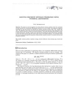
The interval may also be denoted by its center ! nominal value), denoted by the (typically the superscript C, and width (which can be defined by a percentage variation around the nominal value). An interval vector is a vector whose components are interval numbers. A precisely known coefficient has equal left and right limits. When considering interval coefficients for the objective functions only, some approaches use zL and zU, or zL/zU and zC, with the aim of representing the “best” and the “worst” cases. However, this can be misleading if there is a strong correlation between the directions associated with zL and zU (and consequently also zC). In this case it can happen that the convex cone generated by the gradients of zL and zU is “too narrow” and, therefore, only a small part of the non-dominated solution set is reachable. In the limit situation that cone can collapse into a half-ray even though the interval coefficients would enable obtaining wider gradient cones with which more non-dominated solutions could be computed (and are indeed potential solutions to the interval problem). In these situations, in which the gradients of zL and zU are highly ! correlated, relying on them only (or their convex combinations) reduces severely the scope of the search and the number and diversity of solutions that can be computed, as it is illustrated in fig. 3.
Since any realization of the uncertain coefficients can happen, methodological approaches should strive for offering the DM a representative sample of the non-dominated solutions that are attainable with the coefficients within the intervals.
x2
c
c U2
U
cM
L
c2
cL c 1L
c 1U
x1
x2
U
c2 cM 2
cM
L
c2
cU
cL
c 1L
cM 1
c 1U
x1
Figure 3: The consideration of zL and zU only can impair the computation of a representative sample of the non-dominated solutions. The process begins by offering the DM the possibility of freely computing non-dominated solutions in two “extreme” situations: - the “most favorable” objective function coefficients ( c kj = cUkj ,"k, j for functions to be maximized, and c kj = c kjL ,"k, j for functions to be minimized) and the “widest” feasible region L ( A! x " bU where A L = aijL ,"i, j for ≤
[ ]
U
L
[ ]
U U constraints, ! and A x " b with A = aij ,"i, j
for ≥ constraints);
! - the “least favorable” objective function ,"k, j for functions to be coefficients ( c kj = c kjL! ! maximized, and c kj = cUkj ,"k, j for functions to
! !
be minimized) and the “narrowest” feasible region ( AU x " b L for ≤ constraints, and
A L x " bU for ≥ constraints). In particular, the non-dominated solutions that
!individually optimize each objective function !
are computed as well as some well-dispersed solutions with the aim of having a first overview of the non-dominated solution set in these situations. (In the following figures - screen copies - even though the parametric diagrams are totally filled with indifference regions, meaning that all non-dominated basic solutions have been computed, this exhaustive computation is not necessary and, in general, not interesting for the sake of decision support.) The decomposition of the parametric diagram in the “most favorable” (fig. 4) and the “nominal” (fig. 1) situations have the same patterns and all the basic non-dominated solutions are the same. In comparison with the nominal situation, the analysis of the parametric diagram in the “least favorable” situation (fig. 5) reveals that a new basic solution (9) appears modifying the shape of the non-dominated solution set for solutions computed with “balanced” weights. All the other basic non-dominated solutions remain. After this phase, in the computation of each solution, the interval coefficients are randomly generated within their intervals using a uniform distribution. Since all coefficients are randomly changing, basic non-dominated solutions may become dominated, or even infeasible, and new non-dominated solutions may appear. Therefore, a given set of weights in the parametric diagram may belong to indifference regions associated with distinct basic solutions for different coefficient realizations. The indifference regions associated with the non-dominated solutions computed so far are then re-computed using the last iteration random coefficients. The centroid of the indifference region is used as the most stable set of weights leading to that solution. This attempts to capture the fact that the DM “does not choose” scenarios (that is, all realizations of coefficients within the intervals may happen and the DM has no control over it). The method should rather guarantee that a broad diversity of coefficients is (implicitly or explicitly) investigated to assess the robustness of solutions. However, the computer effort required must be taken into account and an exhaustive search is clearly impracticable.
Figure 4: Decomposition of the parametric diagram in the “most favorable” situation.
Figure 5: Decomposition of the parametric diagram in the “least favorable” situation. For each non-dominated basic solution, a robustness index is constructed based on the frequency that basis is generated and the degree of superposition of the indifference regions computed for it with random coefficient realizations within the intervals. For instance, for a random realization of the coefficients within their lower and upper bounds, the decomposition of the parametric diagram displayed in fig. 6 has been obtained. All basic solutions are different from the ones displayed in previous figures, except for solution 3 which has the same basis of solution 6 in the nominal (central coefficients) situation (fig. 1), and solution 2 which has the same basis of solution 9 in the “least favorable” situation (fig. 5). This lack of resilience contributes to degrade
the robustness index of the non-dominated basis computed (for at least a coefficient realization).
intervals. The role of the decomposition of the parametric diagram into indifference regions is to aid the DM in interactively identifying interesting compromise solutions not just regarding the objective functions values but also their robustness to (unknown but bounded) data changes.
Acknowledgements This work has been partially supported by FCT and FEDER under project “Models and algorithms for tackling uncertainty in decision support systems” (POSI/SRI/37346/2001).
References Figure 6: Decomposition of the parametric diagram for random coefficients within the lower and upper limits.
5
Conclusions
Methodological approaches to tackle uncertainty must be at the heart of decision support systems based on multiple objective programming models.
[1] C. H. Antunes, J. Clímaco (1992), Sensitivity analysis in MCDM using the weight space, Operations Research Letters 12, 3, 187-196. [2] C. H. Antunes, J. Clímaco (2000). Decision Aid in the Optimization of the Interval Objective Function. In "Decision Making: Recent Developments and Worldwide Applications", S.H. Zanakis, G. Doukidis, C. Zopounidis (Eds.), 251-261, Kluwer.
Interval programming is a useful approach to model uncertainty, because it does not impose the specification of probabilistic or possibilistic distributions, but just the specification of acceptable left and right limits to the coefficients. This paper reported ongoing research on the development of a decision support tool based on the decomposition of the parametric diagram into indifference regions associated with basic non-dominated solutions.
[3] D. Bertsimas, M. Sim (2004). The price of robustness. Operations Research 52, 35-53.
The parametric diagram provides an interactive visual feedback regarding the superposition of indifference regions corresponding to the same solution, complemented with numerical indicators. This approach of considering in each iteration randomly generated coefficients within the intervals prevents the drawback of other approaches that are based on the extreme rays of the objective functions.
[7] C. Oliveira, C. H. Antunes (2006). Multiple objective linear programming models with interval coefficients – an illustrated overview. Forthcoming in European Journal of Operational Research.
The robustness of these solutions is assessed through a robustness index, which is constructed based on the frequency that basis is computed and the degree of superposition of the indifference regions computed for it with random coefficient realizations within the
[9] Ph. Vincke (1999). Robust solutions and methods in Decision-Aid, Journal of MultiCriteria Decision Analysis 8, 181-187.
[4] Y. Y. Haimes (2004). Risk Modelling, Assessment and Management, Wiley. [5] P. Kouvelis, G. Yu (1997). Robust Discrete Optimization and its Applications. Kluwer. [6] J. Mulvey, R. Vanderbei, S. Zenios (1995). Robust optimization of large-scale systems. Operations Research 43, 264- 281.
[8] B. Roy (1998). A missing link in OR-DA: robustness analysis, Foundations of Computing and Decision Sciences 23, 141160.