the integration process where the individual results are rule sets and the final .... house-votes-84, ionosphere, mushroom, pima-indians-diabetes, tic-tac-toe,.
RULE CONFIDENCE PRODUCED FROM DISJOINT DATABASES: A STATISTICALLY SOUND WAY TO REGROUP RULES SETS Mohamed Aounallah and Guy Mineau Laboratory of computational intelligence, Computer science and software engineering department, Laval University, G1K 7P4, Sainte-Foy, Canada {moaoa, Guy.Mineau}@ift.ulaval.ca
ABSTRACT In this paper, we propose a new technique of distributed data mining which could resolve the problem of having to deal with increasingly bigger databases. We suggest dividing a database into several subsets and processing them in parallel. From these subsets DBi, the technique creates base classifiers in the form of rule sets Ri and extract some other information such as data samples Si, rule generalizations Ri* and rule coverage (i.e., the number of objects classified by the rule) which is used to compute a rule confidence coefficient. With R =∪i (Ri ∪ Ri*) and S = ∪i Si, a binary relation defined over R×S is built, which is used to discriminate between rules (from R) to keep and rules to ignore in order to form the meta-classifier, i.e., the overall classifier. This selection is based on sound statistical measures, thanks to the Central Limit Theorem. KEYWORDS Distributed data mining, data mining, distributed learning, meta-learning.
1. INTRODUCTION: WHY WE NEED DISTRIBUTED DATA-MINING We propose in this paper a solution to resolve the problem of mining increasingly bigger databases. We suggest dividing a database into several subsets which can be processed on different machines. Then individual results are aggregated to produce an abstract view of the whole database. The advantage of processing several relatively small databases is the capacity to process them in parallel on different machines and even on geographically distributed machines. In this case, the individual results, which are in our work in the form of rule sets, have to be merged to produce a unique rule set as if it were produced from the whole database. Obviously, gathering the results can be much faster than gathering the whole data. However, we assume that a unique sub-base can not be representative of the whole database. Indeed, our work deals with the integration process where the individual results are rule sets and the final result, called a meta-classifier, is also a rule set produced by the technique presented in this paper. Other than individual rule sets, this technique relies on rule generalizations, rule error rate and coverage used to compute a rule confidence coefficient, and on very small data samples. Intuitively, rules that form the meta-classifiers are those that have a high confidence coefficient and which classify well the data in the gathered samples. In section 2 a related literature review is presented. Then in section 3, we propose our solution to distributed data mining (DDM). In section 4 we present experimentation results. And finally, we present a conclusion and our future work.
2. EXISTING TECHNIQUES OF DISTRIBUTED DATA MINING There are two classes of distributed data mining techniques: predictive and descriptive. The former is used to predict the class of an unseen object whereas the second one, in addition to the prediction task,
produces an abstract view of the data set by way of a rule set for instance. In the literature there are a lot of techniques that belong to the predictive class such as Stacking (Tsoumakas & Vlahavas 2002), the Arbiter technique (Prodromidis, Chan & Stolfo 2000), the Combiner technique (Chan & Stolfo 1993), the Hybrid technique (Arbiter and Combiner) (Chan & Stolfo 1993), etc. On the other hand, very few techniques belong to the descriptive class. We can cite for instance the Multiple Induction Learning (MIL) algorithm (Williams 1990) (Hall, Chawla, & Bowyer 1998), the distributed learning system (Sikora & Shaw 1996), the fragmentation approach (Cho & Wüthrich 2002), etc. These techniques are the closest to our work. They are all based on the application of a data mining algorithm on different subsets DBi producing different sets of rules Ri. The distributed learning system proposes to regroup rule sets using a genetic algorithm. The MIL algorithm proposes to put together all rule sets then specialize conflicting rules according to their training set. Other rules are added in order to regain the coverage lost by the specialization operation. The main problem of these techniques is the merging process which does not take into account the importance of each set of rules; whereas these sets could be of different importance since the size of the training could be quite different, and so would their coverage. The fragmentation approach, which uses probabilistic rules (Wüthrich 1995), proposes to generate from each data subset DBk a single rule rik for each class Ci. Consequently, for each Ci there exists a rule set concluding on it. This rule set is sorted according to a certain measure, then the top m rules are selected to represent class Ci. The main drawback of this technique is its use of probabilistic rules which supposes that each object attribute possesses a truthfulness probability. In real life, data can not be easily associated with such probabilities and hence this technique could not be used.
3. OUR SOLUTION TO DDM To construct our meta-classifier, we use two types of software agents. The task of the first type of agents is to mine individual data bases; thus we call them miner agents. The second type of agents is called collector agent, where one agent is responsible for aggregating information gathered by miner agents in order to produce the meta-classifier. A detailed description of these agents with justification of our choices follows.
3.1
Mining a data subset
This step is achieved by a miner agent. It produces rule sets characterizing the data set on which it is working (DBi). This is done simply by applying a learning algorithm that could generate a rule set Ri. For instance, we could use any algorithm constructing a decision tree such as CART, ID3 or C4.5, then transform it into a set of rules. In the present work, we chose C4.5 Release 8 (Quinlan 1996) decision tree, which is transformed directly to a set of rules. In addition to rule sets Ri and in order to achieve a more reliable meta-classifier, we have to use other information such as rule generalizations1, their coverage2 and data samples. The reasons that underline the choice of these information are presented below. First, to avoid a characterization which would be too close (too specific) to the data set we propose to use, in addition to rules, their generalizations. In our experimentation we bounded the generalization by removing no more than one predicate thus the number of rule generalizations from one rule with n predicates is n. Since a rule generalization is also a rule, henceforth, the term “rule” will indifferently indicate either a rule or one of its generalizations. Thus, for data subset DBi we would get the following rule set: Ri = {rik | k ∈ [1 .. nri] and nri = ni + gi } where ni is the number of rules and gi is the number of their generalizations. Second, since different rule sets are going to be merged together whereas they are issued from different data subsets and hence each rule has its proper error rate and coverage, we compute for each rule rij a confidence coefficient crij. This coefficient is computed based on a statistical property given by Central Limit theorem (Mitchell 1997) (Roberts 1992). This theorem states that the sum of a large number (≥30) of independent identically distributed random variables follows a distribution that is approximately Normal 1 2
For our purpose, a generalization of a rule is the rule itself with one or more of its predicates absent. The coverage of a rule is the number of items from the training data that it can classify.
(also said Gaussian). Assuming that the error rate is computed over a large number of examples, we can approximate it by a Normal distribution. In other words, if rule error rate Er is computed over a test set containing n examples (n≥30), Er can be approximated by a Normal distribution and hence we can compute the interval (confidence interval) in which will fall the true error rate, i.e., error rate over the distribution (over all unseen objects), in N% of the time as follows: Er ± z n ⋅
Er ( 1 − Er ) n
⇔ Er ± z n ⋅σ
Er
where zn is a constant chosen in regard to N. A table of correspondence between zn and N can be found in almost any statistics books, for instance (Roberts 1992). The term σEr is the error rate standard-deviation. The confidence coefficient of each rule is deduced from the above equation to be one minus the worst error rate that we could compute in N% of the time: crij = (1 - Er - znσEr), i.e., one minus the rule error rate, minus one half the width of the confidence interval of the error rate. The third task of a miner agent, is the extraction of a data sample Si from the data subset DBi. Our sampling is presently done at random. Other sampling techniques are under consideration.
3.2
Aggregation of information gathered and meta-classifier construction
This task is performed by a collector agent. Intuitively, we want to confront each rule generated by each miner agent to data samples gathered from each DBi. Rules that statistically should behave well and which really behave well in the presence of unseen objects (i.e., data samples from other sources) will be kept. The first task of the collector agent is to perform a rule filtering operation based on the rule confidence coefficients: rules having a confidence coefficient lower than a certain threshold t are simply ignored. In other words, collector agent eliminates from R = U i=1…n Ri (where n is the number of data sets) the rules that, based on statistical measures, very much probably will not perform well when faced with unseen objects. The threshold is a parameter we determined empirically. Rules kept form the set Rt. After this rule filtering operation, the collector agent performs a rule selection operation that is based on a binary relation I between objects in S = U i=1…n Si and the rules in Rt. In each intersection rule/object, collector agent writes the following: • 0, if the rule does not cover the object; • 1 or -1 if the object is covered by the rule and is classified correctly or incorrectly, respectively. Based on the binary relation computed above, an error rate can be computed for each rule in Rt considering S as a test set. The error rate of a rule is the number of -1 in its corresponding row in I over the number of non-zero values. Using this error rate, we can evaluate the hypothesis put forth that rules kept in Rt should behave well in N% of the time. Thus the meta-classifier will be composed of all rules in Rt except those that have an error rate over S greater than another threshold tI. As an heuristic, the value of this threshold should be a value around (100-N)%. The resulting meta-classifier is the rule set RtI. Since many rules are ignored in order to form RtI, our technique of meta-classifier production raises the problem of more than one rule is covering the same object. This is a problem when rules are conflicting. In such a case, we apply a majority vote weighed by the confidence coefficient of the conflicting rules. If faced with the equality of the weighted majority vote, we apply a simple majority vote which can also lead, in very rare cases, to a tie. In this ultimate situation, the class of the object could not be predicted and hence we assign to it the majority class in S. Another problem raises when an object may have no rule covering due to rules ignored. To resolve this problem, we simply look for the rules that cover this object within the rules that were ignored. We select the rule that has the highest confidence coefficient.
4. EXPERIMENTATION To assess the performance of our meta-learning, we have tested it on eight data sets: chess end-game (King+Rook versus King+Pawn), house-votes-84, ionosphere, mushroom, pima-indians-diabetes, tic-tac-toe, Wisconsin Breast Cancer (BCW) (Mangasarian & Wolberg 1990), Wisconsin Diagnostic Breast Cancer (WDBC), taken from the UCI repository (Blake & Merz 1998). The size of these data sets varies from 351
objects to 5936 objects. These data sets are firstly divided into two data subsets with a proportion of ¼ and ¾ (as an example, see Figure 1). The first subset is used as test set for the meta-classifier. The second subset is randomly divided into two, three or four data subsets of random sizes, which are divided in turn into two sets with proportion of ⅔ (the .data file in Figure 1 in each DBi) and ⅓ for training and test sets respectively. From the training set a random sample set (the associated .sple file) is extracted with a size of 10% the size of the training set, up to a maximum of 50 objects. This maximum size is needed to bound the method to very small data samples, which is in accordance to one of our goals to minimize processing time. m u s h .d a ta (5 9 3 6 o b je c ts )
m u s h T e s t.te s t ( 1 /4 = 1 4 8 4 o b je c ts )
m u s h T e s t.d a ta ( 3 /4 = 4 4 5 2 o b je c ts ) DB1
DB2
DB3
m u s h 2 .d a ta ( 1 0 9 0 o b j.)
m u s h 1 .d a ta (6 9 0 o b j.)
m u s h 3 .d a ta (1 1 8 8 o b j.)
m u s h 2 .te s t ( 5 4 5 o b j.)
m u s h 1 .te s t ( 3 4 5 o b j.)
m u s h 3 .te s t ( 5 9 4 o b j.)
m u s h 2 .s p le (5 0 o b j.)
m u s h 1 .s p le ( 5 0 o b j.)
m u s h 3 .s p le ( 5 0 o b j.)
Figure 1. Mushroom data base subdivision into training, test and sample sets
For the construction of the base classifiers, we used C4.5 release 8 (Quinlan 1996) which produces a decision tree that we directly transformed into a set of rules. The confidence coefficient of each rule is computed on the basis of 95% confidence interval (i.e., N=95). For threshold tI, we used 5% and 10%, but these two values give exactly the same result. For the threshold t we used • values ranging from 0.95 to 0.20, with decrements of 0.05, • 0.01, •
∑
and µ = 1/ n
n
µi with µi = 1/ nri∑ k =1cr . This threshold is used in order to get a value nri
i =1
ik
without human intervention and which reflects the overall average confidence of the rules. For the evaluation of our method we compared the error rate of the rules it selected (Figure 2, test 4) with, on one hand, the error rate of C4.5 applied on the whole data set (Figure 2, test 1) and on the other hand, the aggregation of all rule sets R (Figure 2, test 2). We also compared the technique with the rule set Rt taken after applying threshold t to R (Figure 2, test 3). All rule sets (“C4.5”, R, Rt and RtI) are tested on the same test set (Figure 2). We have to notice here that the comparison between our method and the C4.5 algorithm is only as a reference because we suppose that we do not have the possibility to gather all the data in the same base. data subset1
∪
data subset2
R1
R2
∪
data subset3
R3
=
aggregation of data subsets
C4.5
R
test set
test 1 test 2
Apply threshold t Rt
test 3
Apply threshold tI R tI
test 4
Figure 2. The battery of tests
4.1
Experimentation results
The first parameter to determine experimentally is the threshold t. To do so, we compute the average error rate over the eight data sets for the four tests (test 1 to 4, Figure 2) when t takes all the values listed above (0.95 to 0.20 and 0.01). Figure 3 represents the corresponding curves where test 1 (C4.5) is represented by lines with diamonds. Test 2 is represented by lines with squares. These two curves are actually straight lines because they are independent from the value of t. Test 3 is represented by lines with X. Test 4 is represented by lines with upper triangles. From Figure 3, we can conclude the following:
1.
Obviously, the best average error rate is obtained by C4.5 algorithm but, as mentioned above, this test could not be done in real life and it is used only as reference. Indeed, we can see that in average R, Rt and RtI are worse than C4.5 by no more than 6% which is a rather acceptable performance. 16 15 14 13 12 11 10 9 0.01
0.2
0.25
0.3
0.35
0.4
0.45
0.5
0.55
0.6
0.65
0.7
0.75
0.8
0.85
0.9
0.95
Figure 3. Average error rate for test 1 to 4 for different values of t
2.
3.
The Rt performance are worse than R performance when t is very low. This is due to some rules which have very low confidence coefficient but which are necessary in the final rule set, when t is low, in order to change the result of the majority vote in the case of conflicting rules. When the value of t is relatively high (≥0.75), Rt gains performance and the filtering process using threshold t gives its fruits. In regard to our statistical hypothesis, only rules with a high confidence coefficient can be considered for the final rule set. The use of RtI practically demonstrate that it can confirm or do not confirm the hypothesis computed for each rule by keeping or eliminating some rules which has as effect a decrease of average error rate of 2% in comparison to Rt. Moreover, when we look to table 2 that represents the size of rule sets R, Rt with t=µ and RtI with tI = 10% and tI = 5%, we can easily conclude that the use of threshold t significantly decreases the rule set size compared to rule set R. In addition, the use of threshold tI decreases, almost in all cases, the rule set sizes compared to that of Rt. The decrease in the rule set size can have a lot of advantages since it decreases the bandwidth use of the meta-classifier and it speeds up the prediction task. Moreover, it facilitates human interpretation of the rule set. Table 2. Number of rules
Data set
Rt (t=µ)
RtI (tI =10%) RtI (tI =5%) BCW 40 13 14 14 Chess 182 77 62 59 Ionosphere 8 5 5 5 Mushroom 12 12 12 12 Pima-Ind. 78 23 11 10 Tic-Tac-Toe 181 56 43 43 Vote 22 12 9 9 WDBC 19 11 11 11 Finally, if t takes the µ value, the average error rate of RtI is 11.6% which is the best average error rate for this rule set and which is better than R and Rt with all t values tested. This could be explained by the fact that µ, as it is an overall average confidence of the rules, finds a consensus over the different data sets to decide of the value deciding of the qualification “good enough to be taken into account”. Considering only RtI with t=µ, when each data set is taken alone, the best error rate that we can get is the same as C4.5 with WDBC data set. The second best error rate is 0.5% worse that C4.5 with mushroom database. This could be explained by the high representation capability of the whole base when each data set is taken alone since the value of µ is very high (0.998) in mushroom database and relatively high in WDBC R
database (0.61). The worst error rate of RtI over eight data sets and when t equals µ is obtained with pimaindians data set with 7.3% worse than C4.5. This is more likely due to the poor representation of the whole data base when each data set is taken alone since the µ value is very low (0.37).
5. CONCLUSION In this paper we proposed a new technique for distributed data mining. This technique is based on a metalearning approach. This technique of meta-learning has the following properties: • Our meta-classifier could be used, not only to classify and predict the class of a new object, but to represent an abstract view of the different data subsets in the form of a rule set. • Thanks to some statistics means, we can associate to each rule computed on the training data sets, a confidence coefficient which will be used to assess its relevance in the creation of the meta-classifier. This confidence coefficient is computed using the error rate and coverage of the rule. This measure is very important since all the rule selection technique is based on it. • Each rule created on one subset is confronted to other subsets in order to assess its statistical validity regarding to new objects. Thus, rules that do not perform well are not kept in the creation of the meta-classifier. • The creation of the meta-classifier is not only based on the rules that classify correctly unseen objects but also takes into account rules that do not perform well in prediction, in order to select those whose performance differs from our expectations. The performance of our meta-classifier is encouraging since, compared to a centralized approach (C4.5), we found that in three cases we have almost the same error rate (less than 1%); in one other case, our metaclassifier performs better; and in the other cases the error rate is worse by at most 8%. All these error rates are computed with randomly generated samples. In order to improve our technique, we are currently studying the effects of the sampling method that produces the Si, the number of subsets and their sizes, etc.
REFERENCES Blake, C., and Merz, C. 1998. UCI repository of machine learning databases. http://www.ics.uci.edu/~mlearn/MLRepository.html. Chan, P.K., and Stolfo, S.J. 1993. Experiments in Multistrategy Learning by Meta-Learning. In Proceedings of the second international conference on information and knowledge management, 314-323. Cho, V., and Wüthrich, B. 2002. Distributed Mining of Classification Rules. Knowledge and information Systems 4:1-30. Hall, L.; Chawla, N.; and Bowyer, W.K. 1998. Combining Decision Trees Learned in Parallel. In Working notes of KDD. Mangasariam, O.L., and Wolberg, W.H. 1990. Cancer diagnosis via linear programming. SIAM News 23(5):1-18. Mitchell, T. 1997. Machine Learning. McGraw Hill. Chapter Evaluating Hypothesis, 128-153. Prodromidis, A.L.; Chan, P.K.; and Stolfo, S.J. 2000. Advances in Distributed and Parallel Knowledge Discovery. AAAI Press / The MIT Press. Chapter Meta-Learning in Distributed Data Mining Systems: Issues and Approaches. Quinlan, J.R. 1996. Improved use of continuous attributes in C4.5. Journal of Artificial Intelligence Research 4:77-90. Roberts, R.A. 1992. An Introduction to Applied Probability. Addison Wesley. Sikora, R., and Shaw, M. 1996. A Computational Study of Distributed Rule Learning. Information Systems Research 7(2):189-197. Tsoumakas, G., Vlahavas, I. 2002. Distributed Data Mining of Large Classifier Ensembles. In Proceedings Companion Volume of the Second Hellenic Conference on Artificial Intelligence, 249-256. Williams, G.J. 1990. Inducing and Combining Decision Structures for Expert Systems. Ph.D. Dissertation, The Australian National University. Wüthrich, B. 1995. Probabilistic Knowledge Bases. IEEE Transactions on Knowledge and Data Engineering 7(5):961:698.