approach to ensure that the application performance meets the .... Controller. Model. Builder. Model: p = f(λ,a). Current resource usage (ut). App-level. SLO (pref).
Runtime Vertical Scaling of Virtualized Applications via Online Model Estimation Simon Spinner and Samuel Kounev University of W¨urzburg
Xiaoyun Zhu, Lei Lu, Mustafa Uysal, Anne Holler and Rean Griffith, VMware, Inc.
Email: {simon.spinner, samuel.kounev}@uni-wuerzburg.de
Email: {xzhu, llei, muysal, anne, rean}@vmware.com
Abstract—Applications in virtualized data centers are often subject to Service Level Objectives (SLOs) regarding their performance (e.g., latency or throughput). In order to fulfill these SLOs, it is necessary to allocate sufficient resources of different types (CPU, memory, I/O, etc.) to an application. However, the relationship between the application performance and the resource allocation is complex and depends on multiple factors including application architecture, system configuration, and workload demands. In this paper, we present a model-based approach to ensure that the application performance meets the user-defined SLO efficiently by runtime “vertical scaling” (i.e., adding or removing resources) of individual virtual machines (VMs) running the application. A layered performance model describing the relationship between the resource allocation and the observed application performance is automatically extracted and updated online using resource demand estimation techniques. Such a model is then used in a feedback controller to dynamically adapt the number of virtual CPUs of individual VMs. We have implemented the controller on top of the VMware vSphere platform and evaluated it in a case study using a real-world email and groupware server. The experimental results show that our approach allows the managed application to achieve SLO satisfaction in spite of workload demand variation while avoiding oscillations commonly observed with state-of-the-art thresholdbased controllers.
I.
I NTRODUCTION
Real-world applications are often subject to time-varying workloads, i.e., the workload intensity and mix change over time, due to seasonal patterns and trends, or unpredictable bursts in user demands. Varying workloads result in frequently changing resource requirements of an application. The traditional approach is to size a system for the expected peak workload. However, this approach suffers from inefficiencies due to the over-provisioning of physical resources and the limited flexibility to cope with unexpected workload bursts. Modern virtualization technologies provide mechanisms for the dynamic provisioning of resources to virtual machines (VMs). These mechanisms can be used to adapt the resource allocation of VMs depending on the current demand. Triggerbased approaches are commonly used in today’s Cloud environments (e.g., Amazon Web Services [1]), where an administrator can specify thresholds on the resource usage and corresponding mitigation actions (e.g., if the CPU utilization is above 80%, start an additional application instance). Many business-critical applications are subject to Service Level Objectives (SLOs) defined on an application performance metric (e.g., latency or throughput). To determine thresholds so that the end-to-end application SLO is fulfilled poses a major challenge due to the non-trivial relationship
between the resource allocation and the application performance. An application administrator has to take into account the following factors influencing the application performance: • Complex application architectures: An application may comprise several tiers, each deployed in one or more VMs. The application latency depends on the processing in each tier and the flow of requests between tiers. Furthermore, asynchronous communication and limited software resources (e.g., thread pools or connection pools) also influence the achievable application performance. • Heterogeneous resource access: The processing of application requests requires access to different types of resources (e.g., CPU, memory, or IO). The extent to which each resource contributes to the end-to-end latency may vary between different application tiers. • Resource contention: Due to the shared nature of a virtualized infrastructure, the achievable performance of one application can be severely impacted by possible resource contention or interference from the co-hosted applications, a problem referred to as noisy neighbors. Furthermore, trigger-based approaches are inherently prone to an oscillating behavior resulting in unnecessary reconfigurations. A system administrator needs to manually find optimal values for various parameters (e.g., frequency of checks, quiet times after reconfigurations) to reduce oscillations. However, the optimal values for these parameters are application-specific and no general guidelines can be determined. In order to overcome the deficiencies of threshold-based approaches and to enable a fully automated approach to dynamically control the resource allocation of virtualized applications, performance models capturing the relationship between the resource allocation to an application and the application performance are required. In this paper, we present a modelbased approach to vertical scaling of virtualized applications at runtime to ensure that the performance of such applications can meet their SLOs. More specifically, we make the following contributions: 1) We propose a layered performance model based on queuing-theory that describes the non-trivial relationship between the application performance and its resource allocation. The performance explicitly captures scheduling delays in the hypervisor. 2) We describe a learning-based approach to automatically estimate this model at runtime based on available monitoring data including aggregate application performance and resource usage statistics. Given that the model is
continuously updated in short time intervals (up to every 5 minutes), it can quickly capture changes in the workload or the configuration of the application. 3) We design a feedback controller that uses the performance model to automatically determine and allocate the number of vCPUs needed by individual VMs in order to fulfill the application SLO. 4) We evaluate the proposed approach using a real-world application and compare its performance with that of a utilization controller that uses a threshold-based scheme. In this paper, we focus on the vertical scaling of individual VMs of an application, where resources are added to or removed from each VM at runtime. Although in virtualized data centers, horizontal scaling would also be feasible by cloning and starting additional VM instances for an application, it typically takes at least minutes for the new instances to be ready. Moreover, it requires the application’s capability to detect and use new instances automatically, which adds additional complexity to the application architecture (e.g., load balancers and session replication mechanisms) and may not be supported by all applications (e.g., database servers). Therefore, the vertical scaling of individual VMs is a viable alternative for virtualized applications as the configured CPU and memory capacity of a VM can be changed quickly and frequently in a hypervisor such as VMware ESX via its hotadd/-remove capability. We have evaluated our approach in a case study based on the Zimbra Collaboration Server [2], a widely used email and groupware application. In the Zimbra experiment, our approach was able to automatically adapt the number of vCPUs of a VM in response to changing resource requirements of the workload. It did this more efficiently and with significantly fewer reconfigurations than a simple threshold-based utilization controller. The remainder of the paper is organized as follows. Section II provides an overview of our model-based approach. Section III discusses the details of our model extraction and updating technique, and Section IV presents the design of the feedback controller that performs automatic vertical scaling of VMs. The experimental setup and the evaluation results are described in Section V and VI. We discuss the related work in Section VII and conclude the paper in Section VIII. II.
can be used to collect the required statistics. For example, VMware Hyperic [3] provides monitoring plugins for a variety of commonly used applications. Our approach is based on a performance model p = f (λ, a) describing the relationship between the application performance p and the current workload λ and resource allocation vector a. The structure and parameterization of the performance model depends on the application architecture. Given that building such a model is a time-consuming task and requires in-depth knowledge of the performance behavior of an application, an automation of the model building process is necessary for the approach to be practically applicable. However, the automatic construction of a fine-grained performance model capturing all performance-influencing factors of an application and the execution environment would require an extensive and detailed instrumentation resulting in high overheads at runtime. Instead, we use a coarse-grained modeling approach where only quickly changing factors (e.g., arrival rates, or scheduling delays at the hypervisor) are captured explicitly. Other factors are assumed to only change slowly around the current operating point over time (over hours and days) and are implicitly integrated in the model parameters. In order to capture changes in these factors, we frequently estimate the model parameters online based on realtime monitoring data. A feedback control loop uses the performance model to adapt the resource allocations to the VMs running the application. To scale a VM vertically we can change the number of vCPUs or the memory size configured for it. Both types of reconfiguration can be done at runtime without the need to restart the VM. Our experiences with ESX show that the CPU/memory resource configurations can be changed within 30 seconds without causing service interruptions in the application. vApp VM1
A virtualized application (referred to as vApp) may comprise multiple VMs running on one or more physical hosts. Each VM may host different parts of an application (e.g., application server or database). We assume that the application owner is able to provide a tuple hmetric, targeti for each vApp specifying the SLO, where metric (denoted as p) defines the application performance metric to be managed (e.g., endto-end latency, or throughput), and target (denoted as pref ) contains the desired value of the corresponding metric. We assume that the user-specified performance metric can be monitored at runtime without significant overheads. Many applications provide these statistics through management interfaces or application logs. Existing monitoring frameworks
...
App Sensor System Sensor
A PPROACH OVERVIEW
In this section, we give an overview of our approach to model-based vertical scaling of VMs. We first describe the basic assumptions behind our approach, and then introduce the feedback control loop for vertical VM scaling at runtime.
VM2
VMn
pt
Application Controller
Observed app Model: p = f(λ,a) performance (pt)
Model Builder Current resource usage (ut)
App-level SLO (pref)
Desired resource allocation (at+1)
vApp Manager
New VM resource settings (number of vCPUs, configured memory size)
Fig. 1.
Overview of the feedback control loop
Fig. 1 gives an overview of the feedback loop. The vApp Manager consists of two modules – the model builder and the application controller. The model builder learns the performance model p = f (λ, a). It receives the current application performance statistics (latency, throughput, and if available the queue length of application requests) from the application sensors and resource usage statistics of all member VMs of vApp from the system sensor. The system sensor leverages the monitoring capabilities of the ESX hypervisor (i.e., from the vCenter PerformanceManager) in order to obtain detailed scheduling statistics. The application controller uses the model to predict the VM-level resource allocation vector at+1 that will be required in the next control interval to fulfill the user-specified performance target pref at the application level. Using hypervisor mechanisms for hot-add of vCPUs and main
memory, the new resource allocation settings are then applied dynamically to the appropriate VMs. The feedback loop is executed at regular time intervals – the control interval – which typically lies in the range of seconds to a few minutes, so that the controller can react quickly to system or workload changes. Our approach considers both, the scale up of VMs in response to an increasing workload intensity as well as the scale down during phases of low usage. While the hypervisor is able to reschedule resources not used by one VM to another, a large VM (i.e., with a lot of configured resources) still causes additional overheads resulting in inefficient usage of physical resources. For instance in the case of CPU resources, the ESX hypervisor implements a co-scheduling (a.k.a. gangscheduling) policy for all vCPUs of one VM. This can result in additional scheduling delays if a VM is assigned several vCPUs. The application controller also determines when the number of vCPUs can be reduced for a VM. In the following, we assume that the total available physical resources of a host are sufficient to fulfill the SLOs of all hosted applications. We consider the problem of performance isolation between applications co-hosted on an over-committed host (i.e., more virtual resources are configured for VMs than there are physical ones available) orthogonal to our problem. In addition, there are two other approaches that can help in this scenario: i) the VMware Distributed Resource Scheduler (DRS) [4] runs every five minutes to automatically migrate some VMs from overloaded hosts to other more idle hosts in the same cluster; ii) the feedback control loop described in [5] can be used to adapt the resource scheduling settings of individual VMs so that the SLOs of high priority vApps can be fulfilled in over-committed scenarios. III.
M ODEL B UILDER
In this section, we first give an overview of how the application and the execution environment are represented in the performance model. We then describe how this performance model is updated at runtime based on monitoring data from the application and system sensors. A. Layered Performance Model The performance model p = f (λ, a) is used to determine a) whether the performance target can be fulfilled under the current workload λ and the current resource allocation a, and b) which resource is currently the performance bottleneck. In order to answer these questions we represent the system with a queueing model. Due to the complexity of virtualized environments, we adopt a layered modeling approach for describing the application performance, where a virtualized system consists of a layered architecture, with each layer contributing to the externally visible application performance. We distinguish between the following three layers, as shown in Figure 2: • The physical resource layer consists of the hardware resources (CPUs, main memory, etc.) of the physical host. • The virtual resource layer consists of the virtual resources (number of vCPUs, size of main memory) which are configured for each VM. The hypervisor dynamically schedules the virtual resources on the physical ones allowing for sharing of physical resources between VMs.
Application layer Virtual resource layer
VM1
vApp
vCPU
Physical resource layer
Fig. 2.
VM2
vCPU Physical CPU
Overview of layered queueing model
• The application layer captures the performance behavior of the application, including software resources (e.g., caches or thread pools) and the control flow between different VMs. Each layer introduces additional sources of contention, which may slow down the processing of application requests. In today’s hypervisors, the physical resources are not dedicated, i.e. the hypervisor dynamically schedules resources to a VM depending on its current demand. In order to increase consolidation ratios and improve resource efficiency, it is possible to over-commit the physical resources of a host. That means, the sum of the configured virtual resources for all the VMs can exceed the capacity of a physical resource of the host. In over-committed scenarios, the different VMs may contend for the same resources at the physical resource layer forcing the hypervisor to time-division scheduling. At the virtual resource layer, different processes may request processing time at resources resulting in delays due to guest operating system scheduling. At the application level, software resources (e.g., thread pools) can lead to software contention limiting the possible application throughput. These different levels contribute to the complex relationship between resource allocation and application performance. In order to address the complexity of the layered architecture of virtualized systems, we adopted a modeling approach based on the Method of Layers (MOL) [6], [7]. MOL is an extension to traditional queueing networks enabling hierarchical modeling. The service time of a queue at level l is equal to the response time of an underlying closed queueing network at level l − 1, i.e., the service times at higher layers include delays due to contention in the lower layers. In the following, we describe the modeling of CPU resources in a virtualized environment. On the application layer, each VM is represented as a M/M/a queue, where the number of servers a corresponds to the number of vCPUs currently assigned to the VM. Depending on the type of application, the scheduling strategy needs to be chosen accordingly. In the following, we assume FCFS scheduling, but the approach can be extended to PS (Processor Sharing)1 scheduling as well. The residence time Rv,a of VM v with a vCPUs is (for a M/M/a/FCFS queue [6]): Qv,a Bv,a ). (1) a Qv,a is the mean queue length seen on arrival of a new request. Bv,a is the probability that a newly arriving request app will find all servers busy. Dv,a is the service demand for processing one request. In the following, this service demand is called application demand in order to distinguish it from the service demands on the virtual and physical resource layers. app Rv,a = Dv,a (1 +
1 Round
robin with infinitesimally small time slices.
Bv,a can be computed using the Erlang C formula [6]. In our experiments, we used the conservative approximation of Bv,a = 1 as we are focused on the high utilization region where newly arriving requests have to wait for service most of the time. The application demand consists of the processing time at different virtual resources (vCPUs and I/O resources) as well as delays due to contention for software resources (e.g., connection pools). In general, the application demand is defined by the function g app (N, D1virt , ..., Dnvirt ), where N is the number of requests being processed concurrently, and Divirt is the service demand of virtual resource i. If assuming detailed knowledge of the application implementation, the function g app could be represented by a queueing model, describing the fine-grained application control flow including accesses to the virtual resources and software resources. However, the operator of a virtualized application usually does not have the necessary knowledge of the application internals to create such a model. In order to avoid the intrinsic complexity of explicitly modeling the application control flow, we chose a coarsegrained modeling approach. Given that we are focused on modeling the vCPU behavior, we do not explicitly model the other resources. Instead, we introduce a general delay resource with IS (Infnite Server)2 scheduling, representing all resources apart from the vCPU. Then the application demand of VM v with a vCPUs is: app virt other Dv,a = Dv,cpu + Dv,a .
(2)
virt Dv,cpu is the service demand at the vCPU, i.e., the CPU time required to process one request. In the following we call it other the virtual resource demand. Dv,a is the time a request spends at other resources in the system. It is assumed that other the value of Dv,a does not change frequently. As described in Section III-B, we continuously update this value to reflect other changes in Dv,a . Equation (2) is valid if the application processes the requests in an FCFS order and the number of requests processed concurrently is less than or equal to the number of vCPUs. If the application is modeled with PS scheduling, delays incurred by the operating system scheduler app due to contention at the vCPU needs to be included in Dv,a .
Changing the number of vCPUs can have a profound impact on the application performance behavior. Therefore, app we expect the application demand Dv,a to change depending value on the number of vCPUs a. For instance, when adding vCPUs to a VM, application thread pools might become a limiting factor due to the increased parallelism resulting in an additional slow-down of the application. Therefore, the app other application demand Dv,a (and also Dv,a ) is learned in relation to the number of vCPUs a. The virtual resource demand is defined as: virt phys Dv,cpu = Wvscheduler + Dv,cpu .
(3)
The time Wvscheduler is the time a request is delayed due to phys is the service VM v waiting for a free physical CPU. Dv,cpu demand at the physical resource layer. This is the CPU time VM v requires to process one request without any contention due to the CPU scheduler in the hypervisor or the operating 2 Ample
servers available so there is no queuing.
system. We call this service demand the physical resource demand. In the VMware ESX hypervisor, there are two main reasons for scheduling delays: over-commitment and co-scheduling. When several VMs require CPU resources at the same time in an over-committed scenario, the hypervisor may be forced to put some of the VMs in a ready state where they wait until a physical CPU becomes available. Furthermore, if a VM has two or more vCPUs, the hypervisor will try to schedule the vCPUs at roughly the same time in order to ensure that the CPU time of the individual vCPUs of the same VM progress simultaneously. If there are not sufficient free physical CPUs to schedule all vCPUs of a VM, the hypervisor may put the VM in a costop state until enough physical resources are available at the same time. While a VM is in the ready or costop state the application processing in the VM is delayed. The delays due to scheduling at the hypervisor layer result in a variable service rate of the vCPU that not only depends on the current application workload of this VM, but the workloads of all other VMs on the same host. B. Model Estimation The parameters of the layered performance model are estimated based on monitoring data provided by the application and the hypervisor. The following parameters are tracked continuously: the application demand, the virtual resource demand, and the physical resource demand. In the following, we describe our approach to estimating these parameters. The estimation of the different demands is based on existing techniques for resource demand estimation (see [8] for an overview of such techniques). However, these techniques do not take the different layers of a virtualized system into account. For instance, the techniques described in [9], [10], [11], [12] are using end-to-end application latency observations. However, as the application latency also includes delays due to contention effects at the hypervisor level, the dynamically changing workload at the hypervisor layer results in unstable demand estimates. The demand estimates are updated in a regular interval, called the estimation interval. At the end of each estimation interval, new readings from the application and system sensors are obtained, and the demand estimates are updated accordingly. For demand estimation only the last M measurements are considered, so that the model estimator can adapt to changes in the system configuration and application behavior. The time period consisting of M measurements is called the estimation window. In our experiments we use an estimation interval of five minutes and an estimation window of one hour. phys The physical resource demand Dv,cpu is estimated based on observations of the average application throughput X and the total CPU execution time crun of a VM v. The value v crun is provided by the ESX hypervisor for each VM. Using v the Utilization Law [13], the following relationship can be assumed: crun phys (4) Dv,cpu = v . L·X v,phys L is the length of the observation period, Dcpu is the physical resource demand, and X is the observed application throughput. In th current prototype, we compute the physical
v,phys resource demand Dcpu using the above equation as an average across the estimation window. If different workload classes are distinguished at the application level, one can use stochastic estimation techniques such as linear regression [14] or Kalman filters [12]).
In order to estimate the virtual resource demand, we rely on scheduling statistics reported by the hypervisor. VMware and ccostop performance counters for ESX provides the cready v v each VM, reporting the total time VM v is in a wait state due to CPU contention from other VMs or due to co-scheduling. This allows us to estimate Wvscheduler , the time a request is delayed due to the VM being in a wait state, similar to the estimation of the physical resource demands: Wvscheduler =
cready + ccostop v v . L·X
(5)
By estimating the wait time Wvscheduler for each estimation interval and combining it with the physical resource demand phys virt Dv,cpu , we obtain the virtual resource demand Dv,cpu . The application demand is estimated based on observations of the residence time Rv,a and the average queue length Qv,a seen by a request on arrival at VM a with a vCPUs. The average queue length Q can either be observed directly if the application provides these statistics or be derived using Little’s Law [13]. Using Equation (1), we can estimate the application app demand Dv,a based on the above observations. We use nonnegative least squares regression to determine the application demand. When we estimate the application demands, we use the previously obtained virtual resource demands and only other estimate the overhead factor Dv,a . So the linear model for the linear regression is: virt Rv,a − Dv,cpu (1 +
Qv,a Qv,a other Bv,a ) = Dv,a (1 + Bv,a ). (6) a a
The linear regression is executed separately for each number app of vCPUs k. The estimation of Dv,a only uses latency Rv,a and queue length Qv,a statistics from estimation intervals with vCPU count a. IV.
R ESOURCE C ONTROL
The layered performance model described in Section III is used to dynamically scale the VMs of a virtualized application in order to ensure application SLOs under dynamically changing workloads. In this section, we describe the resource controller, realized in a model-based feedback control loop. At the beginning of each control interval, the resource controller analyses the layered performance model along with the measured application performance to determine whether VMs need to be scaled up or down, either to mitigate SLO violations or to improve resource efficiency. The current approach is focused on adding and removing vCPUs from individual VMs during system runtime. Changing the number of vCPUs of a VM is a relatively cheap reconfiguration given that modern operating systems support hotplugging of CPU resources without the need to reboot the guest operating system. Thus applications can directly benefit from the additional computing power.
A. Resource Control Algorithm The resource control algorithm is a hill-climbing optimization algorithm executed for each vApp at the beginning of a control interval. Algorithm 1 shows the steps of the algorithm. The algorithm expects the fully-parameterized performance submodels M1 , ..., Mn of each VM, which are created and maintained by the model builder. Additionally, it requires the target application latency Tref as provided by the system administrator, the current arrival rate λ of application requests, and an allocation vector a = (a1 , ..., an ) containing the current number of vCPUs for each VM of a vApp. It returns the desired vCPU allocation vector anext for the next control interval, which is then applied to the system. The algorithm answers (a) whether a reconfiguration is needed to ensure the application performance target, and (b) which VM should be reconfigured. The first part of the algorithm evaluates if the application can still fulfill its performance targets if a vCPU is removed from any of the member VMs and chooses the VM which has the least impact on the application performance (lines 1-12). The second part of the algorithm is executed if the application performance targets are or will soon be violated, and determines which VM is best scaled up to improve the application performance (lines 13-22). In the first step (line 1-4), the performance submodels of each application tier in VM v are analyzed to determine the expected residence time of newly arriving application requests given the current average queue length Qv . The function GetQueueLength (line 2) returns the current number of requests processed or waiting for service in VM v. This value can often be extracted from application log files (e.g., web server access logs or mail server logs). Assuming a stable system within the control interval, it can also be derived based on the observed average arrival rate/throughput and average response time using Little’s Law. The function AnalyseModel takes a performance submodel Mv , the current queue length Qv and the number of vCPUs av for VM v as the input. It then calculates the expected residence time for newly arriving requests using Equation (1) with the current number of vCPUs (line 3) or with one vCPU less (line 4). The function AnalyseModel will return ∞ if av < 1 or av > amax , with amax usually set to the number of physical CPU cores of the host system. This ensures that no infeasible configurations are proposed by the algorithm. In order to determine possible candidate VMs for scale down, the algorithm calculates the expected end-to-end latency Tdown if one vCPU is removed from any of the VMs (line 5 and 6). If the calculated Tdown is less than δ · Tref for any of the VMs, the VM for which removing one vCPU leads to the minimum increase in the end-to-end latency Tdown is selected for scale down. The factor δ is a configurable parameter that controls the aggressiveness with which the controller scales a VM. In the experiments we used a value of δ = 0.75%. Before scale down, an additional check is performed to ensure that the service rate µdown with one vCPU less is sufficient to sustain the current workload (line 9-11). The function GetAppDemand is a helper function that reads the current app value of the application demand Dv,a from a performance model Mv and for a given number of vCPUs a. The stability check avoids unnecessary oscillations, because the queue size would increase again after scale down. This is an issue with
a non-interactive, job-based system (e.g., the mail transfer agent), where it is often acceptable that a certain request queue builds up before the SLO is violated. If there is no potential for a scale-down identified, the controller checks whether a scale-up might be required. First the expected end-to-end latency Tcur for the current arrival rate and current allocation is calculated (line 14) and compared to the target application latency Tref (line 15). Then the algorithm determines the expected speedup s if adding one vCPU to any of the VMs. By scale up of VM v, the speedup s[v] is the ratio between the predicted service rate µup with one additional vCPU and the current service rate µcur (line 19). Then the VM with the highest expected speedup is selected and if the speedup is above a minimum value smin , a vCPU is added. The value smin is configurable and controls how aggressively the controller will scale up a VM. Algorithm 1: Resource control algorithm Input: number of VMs n, target latency Tref , application performance models (M1 , ..., Mn ), arrival rate λ, number of vCPUs (a1 , ..., an ) Output: desired number of vCPUs (anext , ..., anext ) n 1 Data: vectors Rdown , Rcur , Rup , Tdown , s of size n 1 for v = 1 to n do 2 Qv ← GetQueueLength(); 3 Rcur [v] ← AnalyseModel(Mv , Qv , av ); 4 Rdown [v] ← AnalyseModel(Mv , Qv , av − 1); 5 6 7 8 9 10 11 12 13 14 15 16 17 18 19 20 21 22
for v = 1 to n do Pn Tdown [v] ← Rdown [v] + j=1,j6=v Rcur [v]; d ← argmin(Tdown [v]); v if Tdown [d] < δ · Tref then Dapp ← GetAppDemand(Md , ad − 1); 1 µdown ← (ad −1)D app ; if λ < µdown then anext ← ad − 1; d else Pn Tcur ← v=1 Rcur [v]; if Tcur > Tref then for v = 1 to n do app Dcur ← GetAppDemand(Mv , av ); app Dup ← GetAppDemand(Mv , av + 1); app av ·Dcur s[v] ← (av +1)·D app ; up u ← argmax(s[v]); v if s[u] > smin then anext ← au + 1; u
In each control interval, the algorithm adds or removes only one vCPU at a time. This helps the model estimator to learn the application demands Dkapp gradually by exploring the reconfiguration space. In our experiments, the control interval length was set to 20 seconds. With such a short control period, the controller can also react to fast workload changes adequately over several control periods. However, as future work we also plan to support scaling multiple vCPUs per control interval.
B. Bottleneck Analysis While the performance model and the resource control algorithm described previously are focused on capturing changing the number of vCPUs assigned to an application, the model can also be useful to detect non-CPU bottlenecks during runtime and trigger additional reconfigurations. This is especially important if the resource control reaches a point where adding vCPUs will not improve the application performance further. There are different reasons why an application may not benefit from additional vCPUs. In the following, we will discuss possible situations and describe when additional reconfigurations may be necessary. The ESX hypervisor implements a co-scheduling scheme for vCPUs, i.e., all vCPU of the same VM are scheduled roughly at the same time. With increasing number of vCPUs, the probability increases that a VM has to wait because there are less idle physical resources than the VM has vCPUs. Given the current physical demand Dphys and the virtual demand Dvirt , we have an estimate of the time a request is delayed due to hypervisor CPU scheduling. The proportion scheduler can be used as an indicator for excessive ωvirt = W Dapp vCPU contention on a host. If this value reaches a certain threshold (e.g., 30% of the application processing time is due to scheduling delays at the hypervisor level), mitigation actions to reduce the contention on the host can be taken. See [5] on an orthogonal approach optimizing scheduler settings enabling SLO differentiation of virtualized applications. If the physical resources of a host are insufficient to serve the needs of all VMs, it is possible to relocate the VM to a less-utilized host using VM live-migration facilities of the hypervisor (see [4]). other
The proportion ωapp = DDapp can be used as an indicator for either a bottleneck in the application (e.g., insufficient thread pool sizes) or at other hardware resources (e.g., main memory or I/O). In order to pinpoint the bottleneck more precisely, more monitoring data about the current state of the application or hardware might be required. Such metrics may be available as the Zimbra case study in Section VI-D shows. However, the capabilities to solve these bottlenecks during system runtime without service interruption may be limited. C. Reconfiguration We have implemented the resource control algorithm for the ESX hypervisor. The ESX hypervisor currently supports CPU hot-plug, i.e., adding more vCPUs to a VM without service interruptions. However, hot-remove of vCPUs is currently not supported by most guest operating systems. It is necessary to reboot a VM to reduce the number of vCPUs. In order to avoid this limitation, we use CPU hot-plug mechanisms included in some guest operating systems (e.g., the sysfs kernel interface in Linux). We use these mechanisms to deactivate individual cores in the operating system to simulate the influence on the application performance. Given that the hypervisor is not aware of the deactivated cores, these cores may cause additional scheduling overheads in the hypervisor. After a reconfiguration takes place, the model estimator is suspended for a short period of time, because some requests observed directly after the reconfiguration may be enqueued or currently in service during the scale-up/-down. The latencies
E XPERIMENT S ETUP
The Zimbra Collaboration Server [2] is a groupware server based on common open-source components. In this case study, we use the Zimbra server to demonstrate the effectiveness of our queueing-theory-based modeling and the vCPU scaling approach. In order to better understand the performance behavior of Zimbra, we first describe its architecture. Then we describe the experiment setup and our results. A. Zimbra Architecture The architecture of Zimbra is divided into three main components: mailbox server, mail transfer agent (MTA) and LDAP server. Each user of Zimbra has a mailbox on one mailbox server. The mailbox contains the user’s mails, calendars, address books, etc. The user can access the mailbox either using a Web interface provided by the mailbox server through HTTP(S) or using different desktop clients (SOAP, IMAP, or POP3). The mailbox server stores the mailbox data in different locations: a MySQL database containing the meta-data, the content of mails, etc., is stored directly on the file system, and a Lucene search index speeds up content searches. When a user sends a mail, the mailbox server passes it to the MTA that delivers it to the recipient’s server. The MTA may also receive mails from other servers on the Internet. The MTA runs a number of checks on each mail it receives. Most noteworthy are the spam and virus checks. The LDAP server manages the central configuration for multiple Zimbra instances and handles the user authentication. There are different deployment options for these components, ranging from one to three VMs. Each component of Zimbra has a different resource bottleneck. The mailbox server is IO-bound due to database and mail content storage, whereas the MTA is CPU-bound as the virus and spam checks are computationally expensive. Therefore, we choose the VM running the MTA for evaluating the vertical scaling of vCPUs. Although the mailbox server and the MTA can be considered as one application, due to asynchronous communication between them, the processing time at the MTA is excluded in the latency seen by a user. When a user sends a mail, the request returns before the mail is delivered to the recipient. Therefore, it is necessary to also monitor application performance stats at the MTA. Given that Hyperic [3] currently only monitors the queue length of the MTA, we implemented our own application sensor that can also measure the current throughput and latency of the MTA. B. Experiment Setup The experiments are executed using three ESX hosts, ESX1, ESX2, and ESX3, running vSphere 5.1. Each host has the same physical hardware (2.6 GHz Intel Xeon E5430, 32 GB RAM, 150 GB local disk). ESX1 runs a vCenter
For workload generation we use an adapted version of a load driver from the Zimbra performance lab. The driver simulates a session-based, closed workload for a configured number of users. A session consists of several tasks sending requests to the server. Tasks represent atomic user actions (e.g., reading, writing, moving, and deleting mails). The sleep times between the tasks of a session are exponentially distributed. We modified the driver to support dynamic workloads so that it can vary the number of concurrent sessions of users according to a given time series. The mailbox server contained 2500 mailboxes, each with 10MB mail content. We simulated 500 concurrent users. The session intensity was changed every 15 minutes randomly between 1 and 8 sessions per user and per hour. VI.
E XPERIMENT R ESULTS
A. Application Scalability In this experiment, we evaluate the scalability of the application with an increasing workload and number of vCPUs. The workload consists of a fixed number of 500 active users. The session intensity is step-wise increased every hour starting from 2.5 up to 10 sessions per user per hour. The complete experiment run had a duration of 9 hours. The mailbox server is initially configured with 2 vCPUs and the CPU utilization of both cores is below 30%. The bottleneck is the MTA server which is automatically scaled from 1 to 6 vCPUs by our model-based controller in response to the increasing workload. 5 1 vCPU Demand (in seconds)
V.
Server instance, a Hyperic monitoring server, the Zimbra load generator, and our controller. ESX2 runs a VM with the mailbox server and ESX3 runs one with the MTA (both with Linux CentOS 6.4, Zimbra 8.0.5, 4GB RAM and initially 1 vCPU). Mailbox server and MTA are deployed on separate VMs as they can cause high IO rates on the datastore. Given that our prototype currently does not support the control of IO resources, we want to exclude the impact of potential IO contention. The MTA is not connected to the Internet so that only mails from the mailbox server are processed.
2 vCPU
3 vCPU
4 vCPU 5 vCPU
Dphys Dvirt
6 vCPU
4
Dapp a 3 2 1 0
0
Fig. 3.
50
100
150
200
250 300 350 Time (in minutes)
400
450
500
550
Model estimates with increasing workload.
80 1 vCPU CPU time (in seconds)
of these requests are only insufficiently represented by Equation (2) as those requests experienced two different service rates. In order to prevent these observations from influencing the model estimator negatively, we skip all control intervals where the observed average latency T indicates the the requests arrived in the system before the reconfiguration at time tlast (i.e., tcur − T < tlast ).
2 vCPU
3 vCPU
4 vCPU 5 vCPU
6 vCPU
crun ccostop
60
ciowait
40
20
0
0
Fig. 4.
50
100
150
200
250 300 350 Time (in minutes)
400
450
500
ESX scheduling statics during increasing workload.
550
However, the hypervisor co-scheduling overhead is not the only reason for the limited scalability of the MTA. Figure 4 also shows that, the used CPU time (reported by the crun statistic) stagnates with the increasing number of vCPUs. With 6 vCPUs the application could get 120 seconds CPU time in each 20 second interval. However, it is only able to use about 60 seconds of that. To mitigate the bottleneck, a reconfiguration of the application would be required (e.g., changing the number of processing threads in the MTA). B. Physical Resource Contention
Demand (in seconds)
In order to evaluate the impact of physical resource contention on the model estimation, we added additional load VMs to the host where the MTA VM (configured with 2 vCPUs) is running. We used 8 load VMs with 1 vCPU each running a micro-benchmark calculating Fibonacci numbers. These load VMs demand all the physical CPU resources of the host. As a result, the VM running the MTA server is constantly competing for the physical CPU resources and the processing of mails is therefore slowed down in the MTA. No Contention
4
Contention
Dphys Dapp (direct) a
3
Dapp (indirect) a
2
C OMPARISON OF DIRECT TO INDIRECT ESTIMATION OF Daapp FOR A GIVEN V CPU CONFIGURATION No contention Contention
Direct 2.16 3.65
Indirect 2.11 3.65
Relative Error 1.96%


![Why IT Works [PDF]](https://m.moam.info/img/260x300/why-it-works-pdf_647d70d0098a9e6c638b461a.jpg)