Modeling Virtualized Applications using Machine Learning Techniques

Modeling Virtualized Applications using Machine Learning Techniques Sajib Kundu

Raju Rangaswami

Ajay Gulati

Florida International University [email protected]


VMware [email protected]

Ming Zhao

Kaushik Dutta


National University of Singapore [email protected]

Abstract

1. Introduction

With the growing adoption of virtualized datacenters and cloud hosting services, the allocation and sizing of resources such as CPU, memory, and I/O bandwidth for virtual machines (VMs) is becoming increasingly important. Accurate performance modeling of an application would help users in better VM sizing, thus reducing costs. It can also benefit cloud service providers who can offer a new charging model based on the VMs’ performance instead of their configured sizes. In this paper, we present techniques to model the performance of a VM-hosted application as a function of the resources allocated to the VM and the resource contention it experiences. To address this multi-dimensional modeling problem, we propose and refine the use of two machine learning techniques: artificial neural network (ANN) and support vector machine (SVM). We evaluate these modeling techniques using five virtualized applications from the RUBiS and Filebench suite of benchmarks and demonstrate that their median and 90th percentile prediction errors are within 4.36% and 29.17% respectively. These results are substantially better than regression based approaches as well as direct applications of machine learning techniques without our refinements. We also present a simple and effective approach to VM sizing and empirically demonstrate that it can deliver optimal results for 65% of the sizing problems that we studied and produces close-to-optimal sizes for the remaining 35%.

With the proliferation of private and public cloud data centers, it is quite common today, to create or buy virtual machines to host applications instead of physical machines. Cloud users typically pay for a statically configured VM size irrespective of the actual resources consumed by the application (e.g., Amazon EC2). It would be highly desirable for users to size their VMs based on actual performance needs, to reduce costs. At the same time, cloud service providers can benefit from a performance-based charging model built around an application service-level agreement (SLA), thereby eliminating the need for guess work or over-provisioning by the customers [25]. Doing so could increase customer willingness to pay a higher price for better service compared to paying a flat fee based on the size of their VMs. Moreover, cloud service providers would now have the flexibility to dynamically optimize the resources allocated to VMs based on actual demand. The complexity of meeting application-level SLAs and doing performance troubleshooting in virtual environments has been mentioned in many recent studies [15, 21, 32]. The primary source of this complexity lies in finding accurate relationships between resource allocation and desired application performance targets. First, the performance of many real-world applications depend upon the simultaneous availability levels of several resource types, including CPU, memory, and storage and network I/O performance. Performance model are therefore multi-dimensional and complex. Second, while some types of resources (e.g., CPU time, memory capacity) are easy to partition, other types (e.g., storage and network I/O bandwidths) are not. Virtualization magnifies this impact due to the inherent, underlying sharing and contention [21]. Our proposed modeling approach explicitly addresses storage I/O contention, local or networked. We do not address (non-storage) network I/O contention in this work. While host-level NIC bandwidth is typically not a bottleneck, there is little control over inflight packets once they leave the host. Datacenter level solutions are necessary to manage network I/O contention. In this paper, we create per-application performance models that can then be used for VM resource provisioning. Our models use parameters that are based on widely available control knobs for allocating resources to a VM within commodity virtualization solutions. We make the following contributions in this paper. 1. We identify and study the impact of key VM resource allocation and contention parameters that affect the performance of virtualized applications. In doing so, we find that the I/O latency observed by the virtual machine is a good indicator of I/O con-

Categories and Subject Descriptors D.4.8 [Operating Systems]: Performance; C.4 [Performance of Systems]: Modeling techniques General Terms Management, Performance Keywords Virtualization, Cloud Data Centers, VM Sizing, Machine Learning, Performance Modeling

Permission to make digital or hard copies of all or part of this work for personal or classroom use is granted without fee provided that copies are not made or distributed for profit or commercial advantage and that copies bear this notice and the full citation on the first page. To copy otherwise, to republish, to post on servers or to redistribute to lists, requires prior specific permission and/or a fee. VEE’12, March 3–4, 2012, London, England, UK. c 2012 ACM 978-1-4503-1175-5/12/03. . . $10.00 Copyright

Modeling Technique

Strengths

Queueing Theory Control Theory

Usability, Speed Simplicity

Regression Analysis

Usability, Transparency

Bayesian Networks

Extensibility, Transparency

Fuzzy Logic Reinforcement Learning (RL) Kernel Canonical Correlation Analysis (KCCA) Artificial Neural Networks

Extensibility Exploratory

Support Vector Machines

Powerful

Multivariate analysis Powerful

Weaknesses Applications Queuing & Control Theory based Techniques Restrictive assumptions Predicting response times of internet services [14] Computational complexity Linear MIMO models to manage resource for multi-tier applications [26] Machine Learning (ML) Techniques Limited scope Memory resource modeling [35], Translating physical models to virtual ones [36], Fingerprinting problems [10] Binary decisions, DomainFingerpointing for SLA violations [12], Signature construction of systems based history [13] Usability, Stability Predicting resource demand of virtualized web applications [37] Value predictions not supCPU/memory resource allocation for VMs [27] ported Sensitivity to outliers Predict Hadoop job execution time [16] Opacity, Configuration, Computational complexity, Overfitting Opacity, Configuration

Performance prediction for virtualized applications [22]

Workload modeling in shared storage systems [29], Estimating power consumption [24]

Table 1. A compendium of related work on application performance modeling tention in a shared storage environment. We empirically demonstrate that it is possible to model the performance of virtualized applications accurately using just three simple parameters. 2. We apply and extensively evaluate two machine learning techniques, Artificial Neural Network (ANNs) and Support Vector Machine (SVM), to predict application performance based on these parameters. We develop sub-modeling, a clustering-based approach that overcomes key limitations when directly applying these machine learning techniques. 3. We implement and evaluate our modeling techniques for five complex benchmark workloads from the RUBiS [7] and Filebench [2] suites for the VMware ESX hypervisor [33]. The median and 90th percentile prediction errors are 4.36% and 29.17% respectively (averaged across these applications). The higher prediction errors appear mainly within areas of low resource allocation and consequently low performance. 4. We present a simple and effective approach to sizing the resource requirements for VMs in the presence of storage I/O contention based on the performance models that we develop. Our VM sizing experiments deliver optimal results for 65% of the sizing problems that we studied and produces sizes that are close to optimal for the remaining 35%.

2. Background Creating performance models for applications as a function of underlying system parameters is a well researched area. Many previous studies have focused on predicting an application’s performance based on low level performance counters related to cache usage, allocation, and miss rates [14, 28]. Utilizing such models is difficult in virtualized environments because the support of hardware performance counters is not widely available in production hypervisors. However, virtualized environments provide an unique opportunity to model an application’s performance as a function of the size of the VM or underlying hardware resource allocation. The resources allocated to a VM are fungible and can be changed in an online manner. For example, VMware’s vSphere utility allows changing the minimum reservation and maximum allocation or relative priority of CPU, memory, and I/O resources available to a VM at runtime. We now examine the work related to application performance modeling as a function of one or more resources. 2.1

Related Work

We classify the related work into two categories: (1) Queuing & control theory based techniques and (2) Machine learning tech-

niques. Table 1 provides a summary of the related work which we elaborate on below. Queuing and Control Theoretic Models. Doyle et al. [14] used queueing theory based analytical models to predict response times of Internet services under different load and resource allocation. Bennani et al. [9] proposed multi-class queuing networks to predict the response time and throughput for online and batch virtualized workloads. The effectiveness of these solutions is restricted by their simplified assumptions about a virtualized system’s internal operation based on closed-form mathematical models. Another related class of solutions have applied control theory to adjust VM resource allocation and achieve the desired application performance. Such solutions often assume a linear performance model for the virtualized application. For example, firstorder autoregressive models are used to manage CPU allocation for Web servers [23, 34]. A linear multi-input-multi-output (MIMO) model is used to manage the multi-type resources for multi-tier applications [26]. A similar MIMO model is also used to allocate CPU resource for compensating the interference between concurrent VMs [25]. Such linear models are not sufficient to accurately capture the nonlinear behaviors of virtualized applications, which are demonstrated and addressed in this paper. Machine Learning Approaches. Machine learning techniques have been extensively studied for performance analysis and troubleshooting. The CARVE project employs simple regression analysis to predict the performance impact of memory allocation [35]. Wood et al. use regression to map a resource usage profile obtained from a physical system to one that can be used on a virtualized system [36]. However, the accuracy of regression analysis has been shown to be poor when used for modeling the performance of virtualized applications [22]. Cohen et al. [12] introduced Tree-Augmented Bayesian Networks to identify system metrics attributable to SLA violations. The models enable an administrator to forecast whether certain values for specific system parameters are indictors of application failures or performance violations. In subsequent work, the authors used bayesian networks to construct signatures of the performance problems based on performance statistics and clustering similar signatures to support searching for previously recorded instances of observed performance problems [13]. Bodik et al. [10] challenged the usefulness of Bayesian classifiers and proposed logistic regression with L1 regularization to derive indicators. This was shown to be effective for automatic performance crisis diagnosis and in turn facilitating remedial actions. The above techniques address bottleneck identification and forecasting whether certain resource usage and/or application met-

2.2

Building Models

We propose to use advanced machine learning methods to model the relationship between the resource allocation to a virtualized application and its performance using a limited amount of training data. Such a model can then be used to predict the resource need of an application to meet its performance target. One of the questions in this approach is when and how the model is built. Since our approach requires collecting application performance data for a wide range of resource allocation choices, it is difficult to build the model quickly based only on observations from production runs. One option is to have a staging area where a customer can deploy the application and run a sample workload against various resource allocation configurations to facilitate modeling. We can also leverage recent work like justrunit [38] where authors provided a framework for collecting training data by running cloned VMs and applications in an identical physical environment. The modeling techniques that we propose can complement and enhance a such a system which used simple linear interpolation to predict performance results for unavailable allocations.

3. Model Parameters Selection Choosing appropriate control knobs to manage a VM’s resource allocation is critical to create a robust performance model. The purpose of this section is two fold. First we identify the knobs in the form of VM resource allocation parameters that can be used to directly control application performance. Second, we demonstrate that the relationship between these controls and the application performance is quite complex and hard to model.

Normalized Performance Metric

rics would lead to SLA violations. However, they do not address how much SLA violation would be incurred or how resources should be allocated to prevent future violation. In contrast, we specifically address performance prediction: given a set of controllable/observable parameters, what would be the application’s performance? Such prediction can then be used within an optimized resource allocation or VM sizing framework. Xu et al. use fuzzy logic to model and predict the resource demand of virtualized web applications [37]. The VCONF project has studied using reinforcement learning combined with ANN to automatically tune the CPU and memory configurations of a VM in order to achieve good performance for its hosted application [27]. These solutions are specifically targeted for the CPU resource. In addition to CPU, we address memory and I/O contention explicitly. To address such ”what-if” questions, ANN models were proposed in our own previous work [22]. However, subsequent investigations revealed several drawbacks. First, we observed that the parameter to capture I/O contention in shared storage platform can lead to arbitrary inaccuracy in the model (as demonstrated in section 3.3). Second, we observed that the proposed approach of constructing a single model encompassing the entire parameter space in a multi-dimensional model was also severely deficient. In this paper, we propose new modeling techniques that overcome these limitations and evaluate them on a wide set of realistic virtualized server workloads. Further, we demonstrate that our models can also be applied easily for accurate VM sizing. We explore the use of both ANN and SVM approaches to machine learning for performance modeling. Although SVMs are generally applied as a powerful classification technique, SVM-based regression (SVR) is gaining popularity in systems data modeling. In [29], SVR was used to build models to predict response time given a specified load for individual workloads co-hosted on shared storage system. SVR has also been used to model power consumption as a function of hardware and software performance counters [24]. To the best of our knowledge, SVR has not been used before for performance prediction of virtualized applications.

1 0.8 0.6 0.4

RUBiS Browsing RUBiS Bidding Filebench OLTP Filebench Webserver Filebench Fileserver

0.2 0

200

400 800 CPU (MHz)

1000

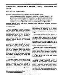
Figure 1. Impact of CPU limit. We focus our discussion on control knobs available on the VMware ESX hypervisor [30]. Similar knobs are available in other hypervisor solutions as well. Throughout this paper, we use five virtualized benchmark applications to both motivate and evaluate our modeling approach. These applications are representative of various enterprise workloads that consume different physical resources (CPU, memory, and I/O) in a complex fashion, and are described in more detail in Section 6. The performance metrics associated with the RUBiS workloads are requests/sec and those for the Filebench workloads are operations/sec. 3.1 CPU Limit ESX provides three control knobs for CPU allocation to VMs: reservation, limit, and shares [31]. Reservation guarantees a minimum CPU allocation expressed in MHz. Limit (in MHz) provides an upper bound on the CPU allocation. Share provides a mechanism for proportional allocation during time periods when the sum of the CPU demands of the currently running VMs exceeds the capacity of the physical host. We chose reservation and limit, both set to the same value as our control knob, to enforce the physical segregation of CPU resources across multiple VMs running on a single physical machine and to ensure that the VM will never get any allocation more than the set value as well. Even with such physical segregation for the CPU, the relationship between application performance and the CPU limit is complex. We measured the performance of the five virtualized applications while varying the VM’s CPU limit from 200 MHz to 1 GHz keeping the memory allocations high enough to ensure that memory is not the bottleneck. We used a VMFS [11] data store on a local disk of the ESX host to store the virtual disks of the VMs. Figure 1 shows the normalized performance of these applications. Both the RUBiS workloads behave non-linearly; the performance slope varies based on CPU allocation ranges. The three personalities of Filebench: OLTP, webserver, and fileserver behave quite differently. While the webserver and fileserver performances saturate quickly at 400MHz, OLTP performance, on the other hand, varies almost linearly with CPU allocation. Overall, this data reveals that virtualized workloads can have quite different performance curves with respect to CPU allocation. 3.2 Memory Limit Similar to the knobs for CPU, the ESX hypervisor provides three controls for memory allocation: reservation, limit, and shares. The semantics of these knobs are similar to the ones for CPU. We set the reservation equal to limit and used this as the control parameter to guarantee a specific memory allocation and no more. Figure 2 shows the normalized performance of these applications as we vary the memory limit from 256 MB to 1 GB. The CPU allocation was kept at a sufficient level to avoid saturation, and there was no I/O contention at the storage. In the case of the



1 0.8 0.6 0.4 0.2 0

RUBiS Browsing RUBiS Bidding Filebench OLTP Filebench Webserver Filebench Fileserver 256 384 512 Memory (MB)

1 0.8 RUBiS Browsing 0.6

RUBiS Bidding

0.4

Filebench OLTP Filebench Webserver

0.2

Filebench Fileserver

0 0

25

50

75 100 Latency (ms)

125

150

1024

Figure 3. Performance impact of VM I/O latency.

Figure 2. Impact of memory limit. I/O Type Seq Seq Seq Rand Rand Rand

Postmark TPS 49 52 46 13 13 11

CDIOPS 6016 8483 8303 154 155 165

I/O latency [ms] 48.08 48.43 46.14 77.14 70.06 81.9

Table 2. Comparison between CDIOPS vs. I/O latency for modeling I/O contention. RUBiS browsing mix workload, performance improves sharply between 256 MB and 512 MB, and remains almost flat afterwards. This behavior can be attributed to the fact that working set size of the workload fits into the memory after a certain allocation. A similar observation can also be made in the case of the RUBiS bidding mix workload, where the working set fits within 384 MB of memory. The Filebench-OLTP workload shows almost no memory dependency and the performance remains flat when the VM’s memory allocation ranges from 256 MB to 1 GB. The performance of the Filebench webserver and fileserver rises gradually as more of the working set fits in memory. Overall, these workloads show varied behavior. Some are insensitive to VM memory allocation, while others show either a sudden or gradual increase in performance as the entire or an increasing fraction of the working set fits in memory. 3.3

Virtual Disk I/O Latency

Strict performance isolation and guaranteed I/O allocation in virtualized environments are challenging because storage arrays are accessed in a distributed manner and the allocation is not under direct control of the hypervisor [17, 18]. I/O allocation can be controlled or modeled in several ways: measuring or controlling the number of I/O operations/sec (IOPS), MB/sec, or I/O latency. In our previous work [22], we used the competing disk IOPS (CDIOPS) issued by other VMs to the shared storage as a measure of I/O contention for a VM. However, there are two main drawbacks to this. First, obtaining the true CDIOPS value when using shared networked storage requires explicit communication either with other hosts or the storage device; this may not be feasible or if so, would incur substantial overhead to keep the information up-to-date. Second, when there is high variance in I/O sizes from competing workloads, the CDIOPS metric can be substantially inaccurate in capturing the actual I/O contention. Large I/O requests would keep the CDIOPS low while causing high device latencies for all VMs. Finally, even the sequentiality characteristics of competing I/O can lead to inaccuracies when using a single CDIOPS value for modeling sequential versus random I/Os which have different costs. To illustrate the limitations of CDIOPS for modeling I/O contention, we ran Postmark [20] in a VM running on a ESX host and generated I/O contention using fio [3] on a different VM. We fixed the I/O size at 4KB and and issued 4 outstanding I/Os at a

time. Keeping the CPU and memory allocation levels constant, we configured the fio VM to issue either random or sequential I/O. We recorded the data for three different instances in each case. Table 2 reports the VM I/O latency, CDIOPS, and the resulting transactions-per-second (TPS) for Postmark. When the competing I/O is sequential, in spite of the higher CDIOPS values, the application performance is better than it is when the competing I/O is random and the CDIOPS values are lower. This simple experiment clearly indicates the inadequacy of CDIOPS as a measure of I/O contention. A similar example can be constructed for bandwidth (in MB/sec) based modeling by using small and large sized I/Os. I/O latency-based measure of I/O contention. We explored the use of the VM I/O latency itself, a direct measure of modeling the I/O performance of a VM in the presence of contention. This metric directly reflects the impact of I/O contention irrespective of its complexity as well as the performance of the underlying device. Table 2 demonstrates that using the VM I/O latency more accurately reflects the performance impact of I/O contention on the Postmark workload. To understand how VMs behave as I/O contention (as captured by I/O latency) varies, we ran each of the five applications in one of the VMs (appVM) and ran the competing fio workload in another VM (called fioVM) both sharing the same storage. The load is varied from the fioVM to create different levels of I/O contention and cause different I/O latencies perceived by the appVM. Figure 3 shows normalized performance as the I/O latency is varied from 20 ms to 120 ms. Most of the applications suffer significant performance degradation when the average I/O latency seen by the appVM increases. The RUBiS Bidding and Browsing workloads generate very few number of I/Os (because their working set is small and fits well in the memory) which made them largely insensitive to the I/O contention. Controlling I/O latency. IO latency observed by a VM can be controlled in many ways. Techniques like PARDA [17] and mClock [18] have been proposed for I/O performance isolation among VMs. With PARDA [17], each virtual disk can be assigned an I/O share value which determines the relative weight of the I/Os from its virtual disk as compared to others. VMs with higher I/O shares get higher IOPS and lower latency. mClock provides additional controls of reservation and limit to control VM latency. Due to a lack of access to these technologies, we used the intensity of contending workloads to control I/O latency for our experiments. Our analysis in this section reveals that the performance of various applications varies in a non-linear and complex manner as the allocation of resources for the VM is changed. We also noticed that the relationship with respect to one resource is dependent on the availability of other resource as well. For example, performance of the RUBiS bidding workload seems almost independent of I/O latency in Figure 3. However, under low memory allocations (256 MB) the performance is impacted by the changes in VM I/O latency. When operating at 256 MB, the performance changed from 1.5 requests/sec under high latency (80-100 ms) to

Benchmark RUBiS Browsing RUBiS Bidding Filebench OLTP Filebench Webserver Filebench Fileserver

% Avg. 68.57 19.30 11.59 19.85 12.89

% Med. 5.23 2.29 8.82 12.88 6.80

Stdev. 119.73 45.86 12.63 30.36 18.64

90p. 340.00 60.18 21.08 38.60 28.78

across the range of output values and higher errors are concentrated in the region with smaller output values. 4.2 Creating Multiple Models with Sub-modeling

Table 3. Prediction errors when using a single ANN Model.

% Error %Error of Prediction

%Error of Prediction

% Error 200 150 100 50 0

200 150 100 50 0

0

20

40

60

80

100

0

20

Sorted Output Points

(a) Single global model

40

60

80

100

Sorted Output Points

(b) Sub models

Figure 4. % Error in prediction for points sorted in increasing order of obtained performance for RUBiS bidding mix. 6 requests/sec under low latency (25-35 ms); an increase of 300%. On the other hand, the performance remains saturates at 59-60 requests/sec when operating under 1024 MB, regardless of the the VM I/O latency level. Such behaviors clearly emphasize the complexity of modeling performance when taking I/O contention into account.

4. Model Design In our previous work [22], we showed the limitations of standard regression analysis techniques for modeling virtualized applications due to their inability to capture the complex behavior; we confirmed these behaviors in the previous section. Specifically, our study demonstrated that the non-linear dependence of performance on resource levels and the complex influence of contention cannot be represented using simple functions. The study also motivated and justified the choice of Artificial Neural Networks (ANN) based modeling for virtualized applications. In this paper, we demonstrate that a simple application of ANN-based technique for modeling can produce large modeling errors when used for complex applications and when possible resource allocations span a wider range (as typical in cloud data centers) than those explored in that study. We introduce the use of another popular machine learning model, Support Vector Machine (SVM) which has gained more popularity recently and find that it has similar limitations as ANN when used directly for modeling. We analyze the root cause of why ANN and SVM techniques are still not sufficient and propose improved use of these tools to substantially increase modeling accuracy. 4.1

Limitations of a Single Global Model

Table 3 summarizes error statistics when using ANNs for modeling a set of workloads. We note that prediction errors can be high in some cases, for instance, the RUBiS workloads. We registered identical observations by applying SVM modeling as well. Further analyzing the data revealed that large errors were mostly concentrated in a few sub-regions of the output value space, indicating a single model’s inability to accurately characterize changes in application behavior as it moves across critical resource allocation boundaries. We demonstrate this behavior in Figure 4(a) where we plot the % error in performance prediction across different testing points of RUBiS bidding mix benchmark (specified by resource allocation and I/O latency levels) when sorted by actual obtained performance in requests/sec. Note that the % errors are quite different

To overcome the limitations posed by a single model, we explored the use of multiple models that target specific regions of the input parameter space. Our proposed sub-modeling technique divides the input parameter space into non-overlapping sub-regions and builds individual models for each sub-region. For performance prediction, the sub-model corresponding to the sub-region containing the input parameters can be used. One approach to sub-modeling is subdividing the space into several equal-sized regions. However, this seemingly simple approach is inadequate. First, it is difficult to determine how many sub-models to use. A small number of submodels may not improve prediction accuracy. Whereas a large number of sub-models would be impractical in terms of collecting sufficient training data points for each to ensure high accuracy. Second, since applications behave non-linearly and non-smoothly with respect to resource allocations, merely building sub-models for equally divided regions may not always be effective in isolating and capturing unique behaviors. To create robust sub-models, we employ classical clustering techniques whereby the data points are separated into clusters based on a chosen indicator parameter. We used an improved version of K-means clustering technique (pamk function in the fpc [4] package of R [6]) that automatically identifies the optimal number of clusters based on the observed values. We used application output values and prediction error values (from using the global model) as two choices for the clustering indicator parameter. To verify that the clustering results were useful, we checked whether the cluster boundaries can be clearly identified based on the input parameter values. In other words, a well-defined cluster should be defined by continuous ranges in the input parameter space. In Section 6, we demonstrate that output-value based clustering indeed produces well-defined regions at the input space with negligible overlapping. After the clustering stage, we segregate the training data points into buckets based on cluster boundaries and build separate sub-models corresponding to each cluster. Predicting for a given resource assignment entails checking the input parameter values and determine which sub-model to use. When clusters do not overlap, for points in the boundary regions, we use ensemble averaging of the two consecutive clusters that these points straddle. If clusters overlap in the input parameters space; we use one of two methods to identify the model to use. The first method uses ensemble averaging of predictions using all the overlapping sub-models. The second method coalesces the overlapping clusters and builds a single sub-model for the merged cluster. In general, for applications with high prediction errors either distributed across the entire parameter space or simply concentrated in a single sub-region, the sub-modeling technique can help reduce prediction errors substantially in comparison to a single global model over both ANN and SVM techniques. We demonstrate the effectiveness of the output value based sub-modeling optimization in Section 6. Apart from evaluating clustering based on output values, we also performed clustering based on prediction error values from the single global model. This choice was motivated by the skewing of high prediction error values towards low allocation values for several of the applications (e.g., in the case of RUBiS bidding mix). At low resource allocation, the sensitivity of the error computation with respect to predicted values is higher when using a single model for the entire range because the application performance drops significantly in this range for most workloads. For instance, requests/sec for RUBiS workloads drops to very low values when the memory assignment of the VM nears 256 MB. Figure 4(a)

(hlayer,hneurons) (1,4) (1,8) (1,12) (2,4) (2,8) (2,12) (2,15) (2,20)

% Avg. Error 13.59 3.25 6.07 6.10 5.17 9.46 2.52 10.34

Std. dev. 13.30 5.43 10.61 9.04 6.12 18.83 3.52 17.48

confirms that the large errors are concentrated in the lower output region of RUBiS bidding mix which corresponds to the application output with less than or equal to 256 MB. We made a similar observation for the RUBiS browsing workload. We created multiple models based on the clustering results on the % prediction error values obtained from the global model. Figure 4(b) demonstrates that error based clustering can substantially reduce the % errors in the lower output regions. In fact, the 90th percentile errors for RUBiS browsing mix dropped from 340% to 27.28%. For the bidding mix, the reduction is from 60.18% to 25.80%. In general, if large errors are concentrated within a specific region of input parameters space, sub-models based on prediction error values from a single global model become valuable. However, this trend does not hold across all the workloads. Except the RUBiS workload mixes, error-based clustering did not lead to well-defined sub-regions and resulted in high overlap in the corresponding input parameter spaces, rendering the clusters practically unusable. On the other hand, sub-modeling based on output values produced robust models across all the workloads we examined. We evaluate output value based sub-modeling in more detail in Section 6.

Table 4. ANN model errors when varying hidden layers (hlayers) and hidden neurons at each layer (hneurons) for the RUBiS bidding mix workload.

5. Model Configuration

Table 5. Errors across individual and ensemble ANN models on RUBiS browsing workload.

In this section, we scrutinize both the ANN-based modeling and SVM-based modeling and identify the key internal parameters that need to be tuned for robust modeling. In addition, we provide details of how the model trainings are performed. 5.1

Model Training

During the training process, a machine learning model gradually tunes its internal network by utilizing the training data set. The accuracy of any model is contingent upon selection of a proper training data set and is evaluated using a different testing data set. Briefly, the training starts with a boot-strapping phase which requires system administrators to identify the best-case and worstcase resource allocation considered feasible across each resource dimension (CPU limit, memory limit, and virtual disk I/O latency) for the workload on the target hardware. The input parameter set is then chosen by first including these boundary allocation values and selecting additional values obtained by equally dividing the range between the lowest and highest values across each resource dimension. This input parameter set and the corresponding output values (obtained by running the workload on the target system) are chosen as the initial training data set. After this initial training, the modeling accuracy with the initial training data set is measured by predicting for the testing data set. If satisfactory accuracy (defined as an administrator chosen bound on prediction error) is achieved, the training process concludes. Otherwise, additional allocation values are computed by preferentially varying highly correlated input parameters (based on the correlation coefficient calculated using any statistical tool) by further subdividing the allocation range with the goal of populating the training set with allocation values that represent the output parameter range more uniformly. 5.2

Model Configuring

We highlight some of the intricacies of model configuration when using ANN and SVM for modeling VM-hosted applications. 5.2.1

Configuring ANNs

Hidden Layer and Hidden Neurons An ANN has multiple layers of neurons which include at least one input layer and one output layer and a tunable number of hidden layers, each with a tunable number of hidden neurons associated with it. The number of hidden layers and hidden neurons at each layer play an integral role in

Model ANN1 ANN2 ANN3 ANN4 ANN5 Ensemble

% Avg. error 64.67 84.62 85.80 58.95 63.09 68.57

% Median error 6.50 9.31 9.68 7.72 8.70 5.23

Std. dev. 105.23 140.82 140.87 107.35 104.93 119.73

determining the accuracy of an ANN model. However, choosing the number of hidden neurons at each hidden layer is not straightforward. If the number of hidden neurons is too small, the model may not assign enough importance to the input parameters and hence suffer from under-fitting. Conversely, if this number is too large, the model may amplify the importance of input parameters and suffer from over-fitting. We evaluated an automated incremental approach of determining the hidden layers and hidden neurons in the training process. We start with one hidden layer and three hidden neurons (because of three input parameters in our environment) at each hidden layer to accommodate the three modeling parameters. We grow the network by adding more neurons on the single hidden layer. We grow the network by adding more layers if we find that increasing number of hidden neurons does not improve modeling accuracy. If adding more neurons or layers does not lead to improved accuracy, we pick the least number of layers/neurons which provided the best accuracy. For an example, the above process led to an ANN configured with 2 hidden layers and 15 hidden neurons at each hidden layer for the RUBiS bidding mix workload. Table 4 summarizes the average and standard deviation of errors for 59 testing data set points using a single global ANN model for RUBiS bidding mix workload under various combinations of hidden layers and hidden neurons at each layer. We applied the same incremental procedure for other workloads to derive the best possible layer/neuron combination for each. Activation Function It defines the mapping function from the input to the output for each node. Our previous study [22] already confirmed that ELLIOT activation function (a faster version of sigmoidal function) is the best choice for this environment. We observed the same trend and hence used ELLIOT activation function for all the benchmarks. Ensemble Averaging Since the initial weight distributions are randomly selected, non-identical models are created across multiple training runs even if the tunable ANN parameters and the training set are the same. We found that the prediction from the testing data can vary significantly across such similarly trained models. One approach to tackle such variability is to generate multiple models and average their predicted output. Such ensemble averaging

using multiple ANN models is a well-known technique which turns out to be quite effective [19]. Table 5 demonstrates how ensemble averaging reduces prediction variability across a set of ANN models generated using the same training data set, training procedure, and identical internal configuration of the ANN. Errors are shown for same testing data points of the RUBiS browsing mix workload. It is important to clarify that ensemble averaging reduces the variations in prediction accuracy across different training runs and does not always deliver to the most accurate predictions. 5.2.2

Configuring SVMs

At high-level, SVM-based regression technique works by first mapping the inputs to a multi-dimensional vector space using some form of non-linear function and finally a linear regression is performed in this mapped space. We specifically used ǫ-regression implementation of e1071 package which provides an interface to the libsvm [5] in R. There are several parameters that need to be tuned for getting accurate modeling with SVM - kernel, gamma, cost. We experimented with a set of kernel functions (linear, polynomial, radial, sigmoid), out of which radial basis function turned out to be effective for our data set. Gamma and cost values were calculated by a tune() function which does a grid search over the training data to figure out the best possible values of those two parameters. It is important to understand the influence of these two parameters, because the accuracy of a SVM model is largely dependent on their selection. For example, if the cost is too large, we have a high penalty for nonseparable points and we may store many support vectors and overfit. Conversely, a very small value may lead to underfitting [8].

6. Evaluation Our evaluation focuses on addressing the accuracy of our submodeling techniques using both the ANN and SVM approaches and contrasting these with regression techniques. We compare each of these modeling techniques when used to create a single global model and as well as clustering based sub-models. We also evaluate the prediction confidence by examining how prediction errors are distributed in the parameter space. Finally, we evaluate the sensitivity of modeling accuracy to training data set size, its robustness to noise in measurements, and the overhead incurred in modeling. For our experiments, we used an AMD-based Dell PowerEdge 2970 server with dual socket and six 2.4 GHz cores per socket. The server has 32 GB of physical memory and ran VMware ESX4.1 hypervisor. All the VMs ran Ubuntu-Linux-10.04. VMs were restricted to use only four of the cores (0-3). All the virtual disks for VMs, and the ESX install were on a VMFS [11] (VMware’s clustered file system) data-store on local 7200 RPM SAS drives from Seagate. We used a VMware vSphere client running on a separate physical machine for managing the resource allocations of individual VMs. The statistics were collected using esxtop utility and transferred to a separate Dell PowerEdge T105 machine with a quad-core AMD Opteron processor (1.15GHz×4), 8 GB of physical memory, 7.2k rpm disk, running Ubuntu-Linux-10.10, for analysis. All modeling tasks were also done using this machine. To simulate I/O contention, we used a separate Ubuntu-Linux VM with 1000 MHz of VCPU and 512 MB of memory to run fio [3] - a Linux-based I/O workload generation tool co-located with the virtualized application being modeled. The number of outstanding I/Os and other workload parameters (e.g., sequentiality) were varied to create different levels of I/O contention on the shared VMFS data-store. A different VM on the same host was used to run Perlbased scripts for changing the allocation parameters for the VMs running the benchmarks. Our choice of following workloads used for evaluation were guided by their representation of data center server workloads and their diversity in resource usage:

Benchmark RUBiS Browsing RUBiS Bidding Filebench OLTP Filebench Webserver Filebench Fileserver

Training points 160 198 135 160 68

Testing points 79 99 75 80 68

Table 6. Training and Testing data set sizes. RUBiS Browsing. A Java servlet based RUBiS [7] Browsing workload was used for the experiments. Client requests were handled by a Tomcat web server and the underlying database was MySQL. The webserver, database, and clients were run on the same VM to minimize network effects that we do not address in this work. 1000 clients were run simultaneously. The Browsing mix consists of 100% read-only interactions. After each run, RUBiS reported average throughput as requests/sec, chosen as the application performance metric. RUBiS Bidding. A similar set up was used for RUBiS Bidding Mix workload with 15% writes. The performance metric was average requests/sec with 400 clients running simultaneously were used and Both the RUBiS profiles are CPU and memory intensive. They generate a small number of I/Os and are largely insensitive to the I/O contention. Filebench OLTP. Filebench [2] is a widely used benchmark for creating realistic I/O intensive workloads such as OLTP, webserver, mail server, etc. We used the Linux based Filebench tool and ran the OLTP application profile which emulates a transaction processing workload. This profile tests for the performance of small random reads and writes, and is sensitive to the latency of moderate (128k+) synchronous writes to the log file. We configured the benchmark to create 32 reader threads and 4 writer threads; I/O size was set to 2KB with a 10GB dataset. We took the Operations per Second (Ops/Sec) reported by Filebench as the application performance metric for this workload. Filebench Webserver. We also used the Webserver profile that performs a mix of open, read, close on multiple files in a directory tree, accompanied by a file append to simulate the web log. We created a fileset of total size 10GB and used 32 user threads. The application performance metric used was the operations per second (Ops/sec) performed. Filebench Fileserver The Filebench Fileserver workload performs a sequence of creates, deletes, appends, reads, writes and attribute operations on the file system. A configurable hierarchical directory structure is used for the file set. Again, we used a dataset of 10GB and 32 simultaneous threads, and used Ops/sec as the application performance metric. 6.1 Modeling Accuracy We evaluated the modeling techniques for overall accuracy across the workloads. Table 6 shows the training and testing data set size used for each benchmark; the training data set was obtained by following the training procedure described in Section 5. A peculiarity of the ANN Elliot function that we use within the core of our ANN models is that it requires the output values to be mapped in the range of 0 to 1. In order to map application performance metric values to this range, we normalized all observed values relative to the observed application performance obtained with the highest resource allocation and no I/O contention and including an additional headroom of 10% to account for outliers. No such translation was necessary for any of the other modeling techniques. We compared the ANN and SVM approaches with the following regression based approaches. Regression linear(L) is the simplest of the regression family which attempts to establish a relationship between the output and the input parameters by considering only first degree terms of the input

Benchmark # clusters % Overlap of consecutive clusters RUBiS Browsing 2 1.25 RUBiS Bidding 4 0.37 Filebench OLTP 8 1.09 Filebench Webserver 2 0.63 Filebench Fileserver 2 1.47

Table 8. Number of clusters and the average % overlap between consecutive cluster pairs, measured using the Jaccard coefficient.

&"!$#

&"!$#

)#

'&!#

'&!#

!#

)%$#

)%$#

&#

!'(#

!'(# !""#

$""#

%""#

&"""#

(a) SVM Sub Model

"# !""#

$""#

%""#

&"""#

(b) ANN Sub Model

variables. Regression quadratic(Q) allows both first order and second order terms for the input variables. Regression linear interactive(LI) captures the combined combined influence of pairs of parameters on the application output (e.g. Memory and I/O Latency) using the first degree of input variables with pairwise interactive terms.

Figure 6. Error Distribution of RUBiS Bidding Mix when using sub models for prediction. The X axis represents CPU Limit (MHz); the Y axis represents Memory Limit (MB). Each box is divided into three columns - representing low, medium, and high (from left to right) VM I/O latency. Error value 0-3% = white, 39% = light grey, 9-27% = dark grey, 27% and more = black.

6.1.1

the other hand, ANN and SVM are able to provide reasonable accuracy in all the scenarios with average errors ranging from 5.90% to 15.95% and 5.65% to 21.51% respectively. To provide a more detailed view of accuracy when using sub-modeling with ANN and SVM, Fig 5 shows the actual and predicted output values for each of the testing points for benchmark. For clarity, we present the actual and predicted values sorted in increasing order of actual performance obtained. Predicted values closely follow the actual values in the majority of the cases.

Single Global Model

Table 7 summarizes the error statistics for all benchmarks and modeling techniques; we focus on average, median, and 90th percentile values of the error distribution. The classical regression techniques largely fail to deliver usable accuracy while using a single global model. This result confirms that the non-linear and non-smooth application behavior cannot be characterized well using simpler mathematical models. Similarly, the ANN global model and the SVM global model also suffer from high average and variance in prediction errors, especially for the RUBiS benchmarks and Filebench webserver, confirming that that global models have limitations when modeling complexity. 6.1.2

Sub-Modeling

Recall that sub-modeling requires clustering of the training data points and then defining cluster boundaries using the corresponding input parameters before creating sub-models for each cluster. Our evaluation focuses on output value based clustering; we found it to be more broadly applicable than error based clustering. We first report the number of clusters and the degree of overlap in consecutive clusters for each benchmark in Table 8. If the total number of clusters is n, the number of consecutive pairs of clusters is n-1. Sub-modeling is only viable when there is less overlap in the input dimensions of the clusters formed. We consider two consecutive clusters overlap only if one or more points in both the clusters overlap in all three input dimensions (CPU, Memory and I/O latency). The output-value based clustering is able to produce well-defined clusters as the average overlaps for all the benchmarks is about 1% as calculated using the Jaccard coefficient. Table 7 presents the error statistics for sub-modeling based on output value clustering for each benchmark. For all workloads and modeling techniques, sub-modeling successfully reduces the mean, median, and 90th percentile of the error distribution when compared to using a single global model. Interestingly, even simple regression models provided greater accuracy using sub-modeling relative to a global model in most cases. This uniform trend clearly indicates that the complexity of these applications cannot be reduced to a single consistent representation as a global model would be forced to adhere to. As the sub models are confined to smaller ranges of the applications performance metric space, they can offer constrained, but more accurate, representations of behavior. Although sub-modeling with clustering increases the attractiveness of simpler regression based models, the power and utility of using the machine learning based models are evident when we consider error variance. We found, in particular, that the effectiveness of regression based modeling is tied to the effectiveness of clustering. When the clusters are bigger, regression models typically perform poorly (average error of 42.78% for R-Browsing using regression-Q) . On

6.1.3

Summary

Based on our analysis with the five virtualized server benchmarks, we conclude that accurately designing and configuring ANN and SVM based models are critical to effectively address the VM performance modeling problem. We find that creating multiple sub models is a necessary step in achieving high accuracy predictions. For instance, even with as few as 68 training data points, both the ANN and SVM based sub-models improve the prediction accuracy for the filebench-fileserver benchmark substantially. In summary, these new techniques substantially improve the prediction accuracy and reduce the average and 90th percentile prediction errors from 26.48% and 101.68% respectively (averaged over all applications) for a correctly configured single ANN global model to 11.04% and 29.17% by using sub-modeling with ANN. Similarly for SVM, the average and 90th percentile prediction errors drop from 34.19% and 66.91% respectively for a single global model to 12.96% and 33.46% using sub models. We also emphasize that between ANN and SVM, there is no clear winner. Although Table 7 shows that ANN is slightly better in prediction statistics than SVM for most of the workloads, these differences are not statistically significant. 6.2 Measures of Confidence While summary error metrics are valuable indicators, the distribution of error values across various combinations of input parameters can be a useful guide to the system administrator while choosing a specific set of allocation values. Particularly, if it is known that in certain regions of the resource allocation space, the modeling error tends to be higher, system administrators can choose to compensate with a greater degree of over-provisioning. Figure 6 shows a heatmap of error distributions for qRUBiS bidding mix workload using SVM and ANN based sub-modeling as an example to illustrate this point. The higher errors are concentrated towards the region of low memory allocations (256 MB) with both techniques, informing administrators of caution while choosing allocations around that range of memory allocations. While we do not address this in our work, it is possible to modify predictions to be conservative for regions prone to higher prediction errors within

Modeling Bench mark RUBiS Browsing RUBiS Bidding Filebench OLTP Filebench Webserver Filebench Fileserver

Regression-L % prediction error avg. med. 90p. 397.08 36.05 1366.83 106.11 17.74 340.60 314.05 30.87 1096.58 9.19 2.43 34.72 18.33 15.75 33.41 6.31 2.74 13.42 76.03 62.99 138.31 32.13 21.85 53.01 49.02 30.70 98.18 21.34 13.63 46.48

Global Sub-Model Global Sub-Model Global Sub-Model Global Sub-Model Global Sub-Model

Regression-Q % prediction error avg. med. 90p. 323.81 23.94 867.77 42.78 4.16 145.01 110.53 21.81 341.54 8.37 1.94 34.64 17.82 12.63 35.58 9.47 3.44 29.48 50.54 44.91 96.71 27.83 20.31 55.09 54.94 21.20 123.36 16.22 8.91 42.64

Regression-LI % prediction error avg. med. 90p. 327.27 35.47 1090.05 103.39 18.78 332.80 317.52 29.37 1126.94 9.10 2.39 35.08 14.02 10.41 28.74 7.55 3.57 10.95 51.44 33.41 113.78 29.85 20.72 55.79 27.59 21.10 55.75 18.35 11.26 38.91

SVM % prediction error avg. med. 90p. 55.78 12.78 142.67 21.51 5.19 68.44 68.86 14.21 100.67 7.38 1.79 22.50 7.40 4.70 13.14 5.65 2.90 15.19 25.02 15.57 53.50 19.38 12.25 36.02 13.87 9.38 24.56 10.89 6.72 25.14

ANN % prediction error avg. med. 90p. 68.57 5.23 340.00 15.95 2.94 45.87 19.52 1.97 80.00 7.18 1.79 30.01 11.59 8.82 21.08 5.90 3.02 13.66 19.85 12.88 38.60 15.57 8.49 33.07 12.89 6.80 28.78 10.60 5.57 23.22

Table 7. % Error statistics (average, median, and 90th percentile) for different modeling techniques by using global models and sub models. ! "#$%&'!(%$)%$!

"**!+%,!-./0'!

120

60

120

100

50

100

80

40

80

60

30

60

40

20

40

10

20

+12!+%,!-./0'!

180

140

160

120

140 100

120 100

80

80

60

60

40

40

20

20

20 0

0 0

40

80

(a) RUBiS Browsing

0 0

50

100

(b) RUBiS Bidding

0

0 0

35

70

(c) Filebench OLTP

0

40

80

(d) Filebench Webserver

0

30

60

(e) Filebench Fileserver

Figure 5. Actual performance and predictions using ANN and SVM based sub-models. The x-axis enumerates data points sorted by increasing performance values. The y-axes represent performance (requests/sec for RUBiS and operations/sec for Filebench respectively).

Error (%)

100 80

Median Error 90th Percentile Error

60 40 20 0 RBOWF RBOWF RBOWF RBOWF RBOWF 20% 40% 60% 80% 100% Fraction of data set used for training

Figure 7. Sensitivity of accuracy to training data set size using ANN based sub-modeling. The x-axis represents the percentage size of final training set and the y-axis represents the median and 90th percentile errors for each benchmark. R-RUBiS Browsing, BRUBiS Bidding, O-Filebench OLTP, W-Filebench Webserver, FFilebench Fileserver. the modeling framework itself once the error distribution is known using a sample set of testing points. 6.3

Sensitivity to the Training Data Set Size

To understand the implications of the training data set size on modeling accuracy, we performed a sensitivity study. We collected a fraction of the final training data set and created sub-models which we then evaluated for prediction accuracy. We repeated the same procedure several times but by changing the fraction of the training set data while retaining the same testing data set each time.

The fractional training data sets were chosen so as to span the output parameter space as much as possible. Figure 7 shows the resulting modeling accuracy for ANN sub-models. We conclude that a careful selection of the fraction of the training data set results in low median errors even when the fraction is as small as 20% for most workloads. The only exception is Filebench Fileserver wherein the total number of points in the training data set was small resulting in only 13 data points in the 20% fractional training set. A similar trend was observed with SVM with sub-modeling. These results indicate that our techniques provide reasonable accuracy even with relatively fewer training data points. 6.4 Robustness to Noise Our experiments thus far were performed in a controlled environment. However, production environments can pose additional challenges, especially with respect to performance variability due to noise. To evaluate the effectiveness of our models in the presence of noise, we simulated noise in 10% of our training data set points. To do so, we perturbed observed performance values by randomly varying these within a fixed percentage specified by the degree of noise. For example, if the degree of noise is 20%, the original value was changed by either +20% or -20%. The testing data set was unmodified across these experiments. In Figure 8, we report the median % modeling errors for each benchmark as we vary the degree of noise when using the ANN-based sub-modeling technique. Trend lines indicate a largely linear dependency between noise and

!"#$%&'()*+,"-%%$%"

'$" '#" *+,-.",/012-34"

'!"

*+,-.",-55-34"

&" %"

6-78983:;"?"

$"

6-78983:;"@8928/A8/"

#"

6-78983:;"6-7828/A8/"

!" !"

#(" (!" )(" '!!"

.+/%++"$0"#$)1+"2!3"

!"#$%&'()*+*+,&'*-$&*+&.$/0&

Figure 8. Change in median error when noise is introduced in the training data set. +" *" )" (" '" &" %" $" #" !"

and memory capacity) that they need to meet application-level performance targets. Given the lack of application-based model customers choose more conservative sizes and over-provision to avoid any performance problems. This leads to sub-optimal sizing and higher costs throughout the life of the VM. A fine-grained, tailored sizing of VMs, on the other hand, can allow meeting target performance while minimizing over-provisioning. In this section, we show that given a target application performance metric and a VM I/O latency level available to the application, our performance models can be used to find the optimal CPU and memory sizes. We used a specific I/O latency as an input because it is not configurable in many cloud environments. However, our modeling can even determine a desired I/O latency value so as to minimize the overall cost of the VM. We experimentally demonstrate that, for a range of performance targets across RUBiS Browsing and Filebench webserver workload, the suggested CPU and memory sizes indeed deliver the required performance in all the cases.

.12&.34&!"#$%&

7.1 VM Sizing Problem Definition

566&.34&!"#$%&

We define the optimal VM sizing problem as follows: Problem definition: Given a performance target Ptarget and a VM I/O latency iolat and a performance model P M , the VM sizing algorithm generates suggested CPU c and a memory m which are able to meet Ptarget and satisfy the following constraints:

Figure 9. Training time. Benchmarks appear in increasing training data set size from left to right

Pc,m,iolat ≥1 Ptarget

(1)

cmin ≤ c ≤ cmax mmin ≤ m ≤ mmax

(2) (3)

subject to: error. Additionally, a key take away from this analysis is that even after 100% modifications of as much as 10% of the training data points, the modeling accuracy does not suffer substantially. In the case of RUBiS bidding workload, the % median error just increased from 1.79% (in case of perfect data) to 2.91% (in case of ±100% change of 10% of the points in the original training data set). In the case of Filebench Webserver, the degradation is from 8.49% to 11.48%. This validates one aspect of robustness under noise as is possible in a production environment. 6.5

Modeling Overhead

Pc−δc ,m,iolat Ptarget