SAFE: a Statistical Algorithm for F0 Estimation for Both Clean and ...

SAFE: a Statistical Algorithm for F0 Estimation for Both Clean and Noisy Speech Wei Chu, Abeer Alwan Department of Electrical Engineering University of California, Los Angeles {weichu, alwan}@ee.ucla.edu

Abstract A novel Statistical Approach for F0 Estimation, SAFE, is proposed to improve the accuracy of F0 tracking under both clean and additive noise conditions. Prominent Signal-to-Noise Ratio (SNR) peaks in speech spectra are robust information source from which F0 can be inferred. A probabilistic framework is proposed to model the effect of additive noise on voiced speech spectra. It is observed that prominent SNR peaks located in the low frequency band are important to F0 estimation, and prominent SNR peaks in the middle and high frequency bands are also useful supplemental information to F0 estimation under noisy conditions, especially babble noise condition. Experiments show that the SAFE algorithm has the lowest Gross Pitch Errors (GPE) compared to prevailing F0 trackers: Get F0, Praat, TEMPO, and YIN, in white and babble noise conditions at low SNRs. Index Terms: fundamental frequency estimation, pitch tracking, noise robust

1. Introduction Accurate F0 tracking in quiet and in noise is important for serveral speech applications, such as speech coding, analysis, synthesis, and recognition. Current F0 tracking algorithms are mainly based on the source-filter theory of speech production and estimate F0 for voiced speech segments. These algorithms usually have two stages. The first stage is to obtain F0 candidates and the likelihood of voicing on a frame-by-frame basis. The second stage is to use dynamic programming to decide the optimal F0 and voicing states for each frame. The F0 candidate generation methods in the first stage can be classified into two categories: singleband and multi-band. In the single-band method, a low-pass filter with a cut-off frequency around 1000 Hz is usually applied to the speech signal before extracting F0 candidates. There are several methods to generate F0 candidates over the voiced speech, e.g. normalized cross correlation function [1], autocorrelation function [2], ’fundamentalness’ based on amplitude and frequency modulation [3], and average magnitude difference function [4]. According to the experimental results in this study, the abovementioned methods can work well under relatively clean conditions. In the multi-band method, a decision module is usually used to reconcile the F0 candidates generated from different bands ([5] [6] [7]). The multi bands used by these methods focus mainly on the low frequency region, i.e. less than 1000 Hz. Supported in part by the NSF.

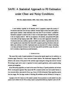
Pre-processing

speech

voicing boundary

voiced frame Y noise N

noise N

Noise Estimation SNR spectrum γ

Spectrum Analysis F0 reference f training

prominent SNR peak Ci

Train or Test?

Peak Analysis frequency l, residual δ, SNR γl , band Bl

Model Learning

F0 candidate f in set SF0 testing

Peak Analysis frequency l, residual δ, SNR γl , band Bl

Bayesian Inference P (f |Ci , N)

residual and SNR distributions: p(δ|γl , Bl , N) and P (γl |Bl , N)

Likelihood Fusion P (f |Y, N)

optimal F0 contour {fˆ1 , fˆ2 , · · · } over frames

Smoothing

Figure 1: A flowchart of SAFE.

Some single-band and multi-band F0 candidate generation methods are also applied to noisy conditions ([8] [9] [10]). Since F0 harmonics in the middle or high frequency regions may not be corrupted by noise (especially babble noise), it is necessary for a noise robust F0 estimation method to utilize this information. Because the reliability of different bands in F0 estimation can vary, it is also necessary to reconcile the F0 estimation results from different bands. Current multi-band methods [5] [7] mainly retain the F0 candidates obtained from the most reliable band, which is a ’hard-decision’, while the Licklider’s pitch perception model uses an empirically-based ’soft-decision’ to merge information from different bands [6]. The proposed SAFE method also adopts a ’soft-decision’ approach, but merges the likelihoods of F0 candidates from different bands in a statistically-based framework. In the following sections, the statistical effects of additive noise on clean voiced speech spectra are studied. This relationship between the noise and information source for F0 estimation is modeled in a probabilistic framework.

2. SAFE: A Statistical Approach for F0 Estimation The flowchart of SAFE is shown in Figure 1.

White noise, SNR=20dB 50

1.6 1.6 1.4

40 SNR (dB)

This paper focuses on estimating F0 values over voiced frames that may be corrupted by quasi-stationary additive noise. Suppose that the range of F0 in human speech is from fmin to fmax , and the frequency resolution of F0 estimation is ∆, SF0 is used to denote the set of all possible F0 values {fmin , fmin + ∆, · · · , fmax }. Given a single observed noisy voiced frame y corrupted by a stationary additive noise n, the probability of f to be F0 of that frame can be expressed as P (f |y, n). The most probable F0 denoted by fˆ should be: fˆ = arg max P (f |y, n) (1)

30 −1.2

20 −1.0 10 0 −10

0

500

Log of the short−term smoothed SNR Log of the long−term smoothed SNR Multiples of the F0 (217.4 Hz) 1.2 0.7 0.9 0.5 1.0 0.5 0.5 0.0 −0.2 −0.4 0.3 −0.9 −0.4 −1.1 −0.5 −0.5 −1.1 −1.3 −1.7

1000

1500 frequency (Hz)

f ∈SF0

P (f |y, n) = P (f |C1 , · · · , CM , N)

(3)

If assuming that the set of local SNR peaks are independent in inferring the F0 given noise shape and level, the overall posterior probability can be presented as a weighted combination of posterior probabilities denoted by P (f |Ci , N): P (f |y, n) =

M X

wi P (f |Ci , N)

(4)

i=1

where wi is the confidence measure of the ith local SNR peak. If each local SNR peak is assumed to have an equal confidence score, then wi can be set to 1/M . As the F0 distribution given the noise, i.e. P (f |N), can be assumed to be uniformly distributed when prior information is not available, P (f |Ci , N) can be calculated according to the Bayesian rule: p(Ci |f, N) f ∈SF0 p(Ci |f, N)

P (f |Ci , N) = P

(5)

The local SNR peak Ci is represented by the following properties: the frequency l, the a posteriori SNR γ l , and the frequency band Bl in which the frequency l is. Because the frequency l does not usually exactly equal to the multiples of F0, l can be decomposed into a multiple m and a residual δ as follows: ˆl˜ l m= (6) , δ = −m f f [ fl

l f

l f

where ] denotes the nearest integer of . If the fraction of is exactly 0.5, it is rounded downwards. Note that the residual ranges from -0.5 to 0.5. Then we have: p(Ci |f, N) = p(m, δ, γ l , Bl |f, N)

(7)

We assume that the deviation of the local SNR peak from a multiple of the F0, caused by noise, will not exceed half F0. Therefore, m is independent of noise N and F0, i.e. P (m|f, N) = P (m|f ). After the decomposition shown in Eq. 6, the residual

2500

3000

White noise, SNR=0dB 30

2.1 2.4 1.9

20

1.5 SNR (dB)

Let Yl and Nl denote the power spectrum of the noisy voiced frame y and noise n at frequency l, respectively. Then the a posteriori SNR at frequency l denoted by γ l is: Yl γ l = 10 log10 (2) Nl As quasi-stationary noise is used in this study, the initial and final frames of noisy speech are used to estimate noisy spectra. The SNR γ l is a measure of the spectral magnitude at frequency l being contaminated by the noise. Obviously, local SNR peaks contain more information than valleys regarding F0. It is assumed that information contained in a set of local SNR peaks denoted by {C1 , · · · , CM } are sufficient for F0 estimation, where M is the number of local SNR peaks. Thus, the posterior probability of F0 is:

2000

10 0

0.5 0.7 −1.4 −0.5 −1.5 −1.2 −0.3 −1.4

0.4 0.7 0.2 0.4 0.2 −0.4 −0.2 0.0 −0.5 −0.3 −0.0 −0.4 −0.9 −0.1 −0.4 −0.5 −1.0

−10 −20

0

500

1000

1500 frequency (Hz)

2000

2500

3000

Figure 2: The SNR spectrum of a voiced frame of a female speaker corrupted by different levels of additive white noise (20 and 0 dB). The number on top of each peak of the short-term smoothed SNR is the value of the normalized difference SNR ζ¯i of that peak li .

δ can be assumed to be independent of m and f given γ l , Bl , and N, i.e. p(δ|m, γ l , Bl , f, N) = p(δ|γ l , Bl , N). The local SNR γ l only depends on the band index Bl and noise condition N, i.e. p(γ l |m, Bl , f, N) = p(γ l |Bl , N). Furthermore, P (m|f ) and P (Bl |m, f, N) are assumed to be uniformly distributed. Then we can have: p(Ci |f, N) = D · p(δ|γ l , Bl , N)p(γ l |Bl , N)

(8)

where D is a constant. 2.1. Prominent SNR Peaks Before studying the distribution of the residual and local SNR peaks, it is important to select useful local SNR peaks for F0 estimation. Two smoothed SNRs denoted by γ Sl and γ Ll are obtained by smoothing γ l with a Hamming window of length fmin and fmax in Hz, respectively. Since the shortterm smoothing can reduce the number of false alarm local SNR peaks and retain F0 information, γ l in Eq. 8 is changed to γ Sl . To depict the relationship between the two smoothed SNRs, an SNR difference at the ith local peak in γ Sl denoted by ζ i can be expressed as follows: ζ i = γ Sli − γ Lli ,

i = 1, · · · , M

(9) γ Sl .

where M is the number of the local peaks in ζ li is further normalized among all the peaks in the frame to be ζ¯i as follows: ζ − µζ ζ¯i = i , i = 1, · · · , M. (10) σζ where µζ and σζ are the mean and standard deviation of the sequence ζ i . The ith local SNR peak is only regarded as a prominent SN R peak for F0 estimation if ζ¯i is above a certain threshold.

As shown in Figure 2, not all local SNR peaks are located in the vicinity of multiples of F0. Most false alarm or deviated peaks have a lower normalized SNR difference compared to the peaks near the multiples of F0. Take the false alarm local peaks around 300 Hz of the voiced frame in Figure 2 for example. These peaks have a lower ζ¯i than the prominent peaks in the two noise conditions. These peaks also have a lower normalized difference SNR compared to their adjacent prominent peaks. The lower a peak is than the long-term smoothed SNR, the more likely it is corrupted by the noise and shifted from its original location, and the less likely it is to be close to the multiples of the F0. Based on this conclusion, only prominent SNR peaks which are less corrupted by the noise and less deviated from the a multiple of F0 can provide reliable information for inferring F0s. As mentioned above, only prominent SNR peaks are used in Eq. 6, i.e. M is reduced to the number of prominent SNR peaks. 2.2. Distribution of the Local SNR and Residual Recall that the residual δ is dependent on the local SNR value and the band index. To reduce the model complexity, it can be assumed that the distribution of the local SNR p(γ l |Bl , N) in Eq. 8 slightly changes when γ l is rounded, i.e.: p(γ l |Bl , N) ≈ p(Qγ l |Bl , N)

(11)

where Qγ l denotes the SNR bin which γ l is rounded to. The distribution can be learned by using a histogram-like approach based on the training set. It can be assumed that this rounding does not significantly change the distribution of the residuals p(δ|γ l , Bl , N), i.e.: p(δ|γ l , Bl , N) ≈ p(δ|Qγ l , Bl , N)

(12)

Curve-fitting or Gaussian mixture modeling can be used to model the distribution of the residuals; however, it is important to control the number of parameters in the model which enables training with limited data and prevents model overfitting. Doubly truncated Laplace distribution denoted by p(δ|µ, b) is used for modeling the p(δ|Qγ l , Bl , N), i.e. the distribution of residuals given the rounded SNR bin, band index and noise condition: ( “ |δ − µ| ” A 1 1 − ≤δ≤ exp − p(δ|µ, b) = 2b b 2 2 (13) 0 otherwise where µ and b represent the mean and variance, respectively. A R is set to be (1 − e−1/2b )−1 to ensure δ p(δ|µ, b) = 1. Only two free parameters (µ, b) are estimated. Given a sequence of residuals {δ1 , · · · , δN } denoted by ∆, suppose all the residuals are i.i.d., we have: p(∆|µ, b) =

N Y

p(δi |µ, b)

(14)

i=1

Let α = 1/2b and L(∆|µ, α) = log p(∆|µ, b), then: L(∆|µ, α) = N log α − N log(1 − e−α ) − 2α

N X

|δi − µ| (15)

i=1

Under the maximum-likelihood criterion, the estimated mean and variance denoted by µ ˆ and ˆb (or α ˆ ) should maximize the joint probability p(∆|µ, b) which is equivalent to maximizing the L(∆|µ, α). P Since ∂ 2 L/∂µ2 = −2α N i=1 δ(δi − µ) ≤ 0 when α > 0, L(∆|µ, α) with a fixed α > 0 achieves its maximum when

∂L/∂µ = 0, i.e.: −2α

N X

sgn(δi − µ ˆ) = 0

(16)

i=1

Since ∂ 2 L/∂α2 = eα /(eα −1)2 −1/α2 < 0 when α > 0, L achieves its maximum when ∂L/∂α = 0 and µ = µ ˆ, i.e.: N 1 1 2 X |δi − µ ˆ| = 0 − αˆ − α ˆ e −1 N i=1

(17)

Although there is no close-form solution to Eqs. 16 and 17, Newton’s method can be used to search for µ ˆ and α. ˆ Note that ˆb = 1/2α. ˆ When a bin with a high rounded SNR does not have training instances, no effort of running the mean and variance solvers is spared. In case some unseen residuals might have higher SNRs, the mean is set to 0, and the variance is set to a small value, e.g. 0.01. While the curve-fitting approach might result in a model of high complexity and be over-fitted to the training data, our mathematical modeling approach can avoid these problems by using prior knowledge about the shape of distribution. 2.3. Post-Processing For an utterance, the posterior probabilities, i.e. P (f |y, n) on each frame is obtained by calculating Eqs. 8 and 4. A dynamic programming approach is used to not only smooth the tracked F0 contour but also to allow octave jumps at a certain cost [1]. The focus of the proposed method is to reduce the F0 estimation error under both clean and noisy conditions. However, the voicing boundary can affect the results of F0 tracking [11]. To eliminate the uncertainty introduced by voicing decision errors, the ground truth of voicing information is used. That means that the different F0 tracking algorithms estimate F0 values over all voiced frames regardless of their SNRs.

3. Experiments Gross Pitch Error (GPE) [12] (±20% allowable deviation from the ground truth) is used to evaluate the performance of F0 estimation algorithms. In this section, we compare the GPE using the KEELE [13] and FDA [14] corpora. The 5 minute 37 second KEELE corpus contains a simultaneous recording of speech and laryngograph signals for a phonetically-balanced paragraph which was read by 5 male and 5 female speakers. The 5 minute 32 second FDA corpus is composed of laryngograph and speech signals from one male and one female speaker. Each speaker read 50 sentences in the FDA corpus. Ground truth F0s were obtained by running an autocorrelation method on the laryngograph signal in addition to some manual correction ( [13] [14]). Speech signals are downsampled from 20000 Hz to 16000 Hz for both corpora. Noise is artificially added to the corpora to test the robustness of the F0 trackers under different noise conditions. The program FaNT was used to employ white and babble noise segments from the NOISEX92 corpus to generate utterances with SNR of 20, 10, 5, 0, and -5 dB [11]. The parameters of SAFE are as follows: FFT size is 16384; frequency resolution is 1 Hz; frame length and step size are 0.04 and 0.01 seconds, respectively; fmin and fmax are 50 and 400 Hz, respectively; the lengths of the short-term and longterm windows for spectrum smoothing are 50 and 400 in Hz, respectively. A peak is regarded as a prominent peak if the normalized difference SNR ζ¯i is greater than an empirically de-

termined threshold of 0.33; the ranges of the low, middle, and high frequency bands are 0-1, 1-2, and 2-3 kHz, respectively; local SNRs of the peaks are rounded to the nearest value in the following sequence 10r/3, where r = 0, 1, · · · , 21. For the KEELE corpus, a 5-fold cross-validation scheme is applied. For each fold under a certain noise level, the speech of one male and one female speaker are used for testing, the residual and SNR models are trained from the remaining speech and its ground truth. Since 54% of the KEELE corpus is voiced speech, if the frame step size is 0.01 seconds, each fold has about 14000 frames for training. Since there are 23 rounded local SNR bins, if each voiced frame has 10 prominent peaks on average, each residual model has about 6000 samples for training. Because some bins with high SNRs might have fewer training instances, e.g. 5% of the average - 300 samples, it is still possible to robustly train a doubly-truncated Laplace distribution with only two free parameters. To determine the generalizablity of SAFE, the model trained from the KEELE corpus is used for the FDA corpus. The GPE comparison of the Get F0 [1], Praat [2], TEMPO [3], YIN [4], and proposed SAFE on KEELE corpus is shown in Table 1. All F0 trackers perform well under clean conditions with GPEs lower than 3.5%. All algorithms suffer from performance degradation when the SNR drops. As expected, it is more difficult to accurately estimate F0 under babble noise condition compared to white noise with the same SNR. The SAFE algorithm has the lowest GPE when the SNR is at or below 5 dB under white noise, and at or below 10 dB under babble noise. We also ran experiments where only the low frequency band (0-1 kHz) was used in SAFE. The GPE of SAFE with only low-frequencies is higher than the standard SAFE, but still lower than other F0 tracking algorithms in low SNR conditions. Although there is a mismatch between the KEELE and FDA corpora, SAFE still has the lowest GPE on FDA under low SNR conditions as it does for the KEELE corpus.

Table 1: The GPE (%) of the Get F0, Praat, TEMPO, YIN, and SAFE using the KEELE and FDA corpora. Bold numbers represent the lowest GPE in each column.

SNR (dB)

Clean

20

Get F0 Praat TEMPO YIN SAFE

2.62 3.22 2.98 2.94 2.98

2.69 3.16 3.41 2.94 3.01

Get F0 Praat TEMPO YIN SAFE Get F0 Praat TEMPO YIN SAFE Get F0 Praat TEMPO YIN SAFE

2.87 3.18 4.69 3.27 3.10 2.45 2.27 2.27 2.25 2.40

2.46 2.27 2.29 2.25 2.41 2.86 2.65 3.56 2.36 2.61

10 5 0 KEELE White Noise 3.10 4.09 7.69 4.28 6.11 11.53 4.27 5.57 12.79 3.20 3.96 6.70 3.35 3.66 4.06 KEELE Babble Noise 7.19 15.99 29.76 8.33 17.97 35.26 13.99 26.98 43.98 8.89 19.71 36.75 4.72 7.44 15.88 FDA White Noise 3.04 3.94 6.73 2.99 4.35 11.84 2.87 5.07 11.64 2.36 3.34 5.20 2.69 3.10 3.24 FDA Babble Noise 8.36 24.41 46.41 10.55 27.15 46.32 15.24 33.10 54.43 10.09 27.53 51.15 4.14 7.73 19.32

-5 17.83 30.91 22.64 14.48 5.01 58.40 54.06 65.15 57.35 39.23 17.72 27.54 31.65 12.33 3.68 64.52 64.24 66.38 68.22 57.17

[6] A. de Cheveigne, “Speech F0 extraction based on Licklider’s pitch perception model,” ICPhS, 1991, pp. 218–221.

4. Conclusions

[7] F. Sha, J. Burgoyne, and L. Saul, “Multiband statistical learning for F0 estimation in speech,” ICASSP, 2004, vol. 5, pp. 661–664.

Prominent Signal-to-Noise Ratio (SNR) peaks constitute a simple and an effective information source for F0 inference under both clean and noisy conditions. The statistical framework of F0 estimation is promising in modeling the effect of additive noise on the clean speech spectra given F0. In addition to low frequencies, middle and high frequency bands (1-3 kHz) provide supplemental useful information for F0 inference. The proposed SAFE algorithm is more effective in reducing the GPE compared to prevailing F0 trackers especially for low SNRs.

[8] D. Krusback and R. Niederjohn, “An autocorrelation pitch detector and voicing decision with confidence measures developed for noise-corrupted speech,” IEEE Trans. on Signal Processing, vol. 39, no. 2, pp. 319–329, 1991.

5. References [1] D. Talkin, “Robust algorithm for pitch tracking,” Speech Coding and Synthesis, pp. 497–518, 1995. [2] P. Boersma, “Praat, a system for doing phonetics by computer,” Glot International, vol. 5, no. 9/10, pp. 341–345, 2001.

[9] T. Nakatani and T. Irino, “Robust and accurate fundamental frequency estimation based on dominant harmonic components,” JASA, vol. 116, no. 6, pp. 3690–3700, 2004. [10] O. Deshmukh, C.Y. Espy-Wilson, A. Salomon, and J. Singh, “Use of temporal information: Detection of periodicity, aperiodicity, and pitch in speech,” IEEE Trans. on Speech and Audio Processing, vol. 13, no. 5, pp. 776–786, 2005. [11] W. Chu and A. Alwan, “Reducing F0 frame error of F0 tracking algorithms under noisy conditions with an unvoiced/voiced classification frontend,” ICASSP, 2009, pp. 3969–3972. [12] L. Rabiner, M. Cheng, A. Rosenberg, and C. McGonegal, “A comparative performance study of several pitch detection algorithms,” IEEE Trans. on Acoustics, Speech, and Signal Processing, vol. 24, no. 5, pp. 399–418, 1976.

[3] H. Kawahara, H. Katayose, A de Chevigne, and R. Patterson, “Fixed point analysis of frequency to instantaneous frequency mapping for accurate estimation of F0 and periodicity,” EUROSPEECH, 1999, vol. 6, pp. 2781–2784.

[13] F. Plante, G. Meyer, and W. A. Ainsworth, “A pitch extraction reference database,” EUROSPEECH, 1995, pp. 837–840.

[4] A. de Cheveigne and H. Kawahara, “YIN, a fundamental frequency estimator for speech and music,” JASA, vol. 111, no. 4, pp. 1917–1930, 2002.

[14] P.C. Bagshaw, S.M. Hiller, and M.A. Jack, “Enhanced pitch tracking and the processing of F0 contours for computer aided intonation teaching,” EUROSPEECH, 1993, vol. 2, pp. 1003–1006.

[5] M. Lahat, R. Niederjohn, and D. Krusback, “A spectral autocorrelation method for measurement of the fundamental frequency of noise-corrupted speech,” IEEE Trans. on Acoustics, Speech, and Signal Processing, vol. 35, no. 6, pp. 741–750, 1987.