using unmanned aerial systems (UASs) for civil purposes. The applications of ... collision avoidance [15], automated in-flight refueling [20], and many others [21], ...
Safe Sequential Path Planning of Multi-Vehicle Systems Under Disturbances and Imperfect Information Somil Bansal*, Mo Chen*, Jaime F. Fisac, and Claire J. Tomlin Abstract— Multi-UAV systems are safety-critical, and guarantees must be made to ensure no undesirable configurations such as collisions occur. Hamilton-Jacobi (HJ) reachability is ideal for analyzing such safety-critical systems because it provides safety guarantees and is flexible in terms of system dynamics; however, its direct application is limited to smallscale systems typically of no more than two vehicles because of the exponentially-scaling computation complexity. By assigning vehicle priorities, the sequential path planning (SPP) method allows multi-vehicle path planning to be done with a computation complexity that scales linearly with the number of vehicles. Previously the SPP method assumed no disturbances in the vehicle dynamics, and that every vehicle has perfect knowledge of the position of higher-priority vehicles. In this paper, we make SPP more practical by providing three different methods for accounting for disturbances in dynamics and imperfect knowledge of higher-priority vehicles’ states. Each method has advantages and disadvantages with different assumptions about information sharing. We demonstrate our proposed methods in simulations.
I. I NTRODUCTION Recently, there has been an immense surge of interest in using unmanned aerial systems (UASs) for civil purposes. The applications of UASs extend well beyond package delivery, and include aerial surveillance, disaster response, and other important tasks [1]–[5]. Many of these applications will involve unmanned aerial vehicles (UAVs) flying in an urban environment, potentially in close proximity of humans. As a result, government agencies such as the Federal Aviation Administration (FAA) and National Aeronautics and Space Administration (NASA) of the United States are urgently trying to develop new scalable ways to organize an air space in which potentially thousands of UAVs can fly together [6]– [8]. One essential problem that needs to be addressed is how a group of vehicles in the same vicinity can reach their destinations while avoiding collision with each other. In some previous studies that address this problem, specific control strategies for the vehicles are assumed, and approaches such as induced velocity obstacles have been used [9]–[11]. Other researchers have used ideas involving virtual potential fields to maintain collision avoidance while maintaining a specific formation [12], [13]. Although interesting results emerge This work has been supported in part by NSF under CPS:ActionWebs (CNS-931843), by ONR under the HUNT (N0014-08-0696) and SMARTS (N00014-09-1-1051) MURIs and by grant N00014-12-1-0609, by AFOSR under the CHASE MURI (FA9550-10-1-0567). The research of M. Chen and J. F. Fisac have received funding from the “NSERC” program and “la Caixa” Foundation, respectively. * Both authors contributed equally to this work. All authors are with the Department of Electrical Engineering and Computer Sciences, University of California, Berkeley. {somil, mochen72, jfisac, tomlin}@eecs.berkeley.edu
from these studies, simultaneous trajectory planning and collision avoidance were not considered. Trajectory planning and collision avoidance problems in safety-critical systems have been studied using reachability analysis, which provides guarantees on the success and safety of optimal system trajectories [14]–[19]. In this context, one computes the reachable set, defined as the set of states from which the system can be driven to a target set. Reachability analysis has been successfully used in applications involving systems with no more than two vehicles, such as pairwise collision avoidance [15], automated in-flight refueling [20], and many others [21], [22]. Despite the advantages of reachability analysis, it cannot be directly applied to complex high dimensional systems involving multiple vehicles. Reachable set computations involve solving a Hamilton-Jacobi (HJ) partial differential equation (PDE) on a grid representing a discretization of the state space, causing computation complexity to scale exponentially with system dimension. In [23], the authors presented sequential path planning (SPP), in which vehicles are assigned a strict priority ordering. Higher-priority vehicles ignore the lower-priority vehicles, who must take into account the presence of higherpriority vehicles by treating them as induced time-varying obstacles. Under this structure, computation complexity scales just linearly with the number of vehicles. In addition, a structure like this has the potential to flexibly divide up the airspace for the use of many UAVs; this is an important task in NASA’s concept of operations for UAS traffic management [8]. The formulation in [23], however, ignores disturbances and assumes perfect information about other vehicles’ trajectories. In presence of disturbances, a vehicle’s state trajectory evolution cannot be precisely known a priori; thus, it is impossible to commit to exact trajectories as required in [23]. In such a scenario, a lower-priority vehicle will need to account for all possible states that the higher-priority vehicles could be in. To do this, the lower-priority vehicle needs to know the control policy used by each higher-priority vehicle. Unfortunately, perfect information about other vehicles’ control strategies cannot be realistically assumed. Thus, in order for any path planning scheme to be viable, perfect information cannot be assumed, and disturbances must be accounted for. The main contribution of this paper is to take advantage of the computation benefits of the SPP scheme while resolving some of its practical challenges. In particular, we achieve the following: • incorporate disturbances into the vehicle models, • analyze three different assumptions on the control strat-
•
egy information to which each vehicle may have access to, for each assumed information pattern, we propose a reachability-based method to compute the induced obstacles and the reachable sets that would guarantee collision avoidance as well as successful transit to the destination.
𝒯2
𝑄3
𝒯1 𝑅𝐶 𝑄1 Targets Vehicle Danger zone
𝒯3
𝑄2
II. P ROBLEM F ORMULATION Consider N vehicles, denoted Qi , i = 1, . . . , n, whose dynamics are described by the ordinary differential equation x˙ i = fi (t, xi , ui , di ), ui ∈ Ui , di ∈ Di ,
t≤
tSTA i
i = 1, . . . , N
(1)
where xi ∈ Rni , ui denote the state and control of ith vehicle Qi respectively, and di denotes the disturbance experienced by Qi . In general, the physical meaning of xi and the dynamics fi depend on the specific dynamic model of Qi , and need not be the same across the different vehicles. tSTA i in (1) denotes the scheduled time of arrival of Qi . We assume that the control functions ui (·), di (·) are drawn from the set of measurable functions1 . In addition, we assume that the disturbances di (·) are drawn from Γ, the set of non-anticipative strategies [15], defined as follows: Γ := {N : Ui → Di | ui (r) = u ˆi (r) a. e. r ∈ [t, s] ⇒ N [ui ](r) = N [ˆ ui ](r) a. e. r ∈ [t, s]}
(2)
For convenience, we will use the sets Ui , Di to denote the set of functions from which the control and disturbance functions ui (·), di (·) can be drawn. We assume that fi (t, xi , ui , di ) is bounded, Lipschitz continuous in xi for any fixed t, ui , di , and measurable in t, ui , di for each xi . Thus, given any initial state x0i and any control function ui (·), there exists a unique continuous trajectory xi (·) solving (1) [24]. Let pi ∈ Rp denote the position of Qi ; note that pi in most practical cases would be a subset of the state xi . Denote the rest of the states hi , so that xi = (pi , hi ). Prior to its departure, each vehicle Qi is assumed to be at the state xi0 . Under the worst case disturbance, each vehicle aims to get to some set of target states, denoted Ti ⊂ Rni , at some scheduled time of arrival tSTA i . On its way to Ti , each vehicle must avoid the danger zones Aij (t) of all other vehicles j 6= i for all time. In general, the danger zone can be defined to capture any undesirable configuration between Qi and Qj . In this paper, we define Aij (t) as Aij (t) = {xi ∈ Rni : kpi − pj (t)k2 ≤ Rc },
(3)
the interpretation of which is that a vehicle is in another vehicle’s danger zone if the two vehicles are within a Euclidean distance of Rc apart. The joint path planning problem is depicted in Fig. 1. 1 A function f : X → Y between two measurable spaces (X, Σ ) and X (Y, ΣY ) is said to be measurable if the preimage of a measurable set in −1 Y is a measurable set in X, that is: ∀V ∈ ΣY , f (V ) ∈ ΣX , with ΣX , ΣY σ-algebras on X,Y .
Fig. 1: Problem setup. The problem of driving each of the vehicles in (1) into their respective target sets Ti P would be in general a differential game of dimension i ni . However, due to the exponential scaling of the complexity with the problem dimension, an optimal solution is computationally intractable even for N > 2, with ni as small as 3. In this paper, we assume assigned priorities of the vehicles as in the SPP method [23]. While traveling to its target set, a vehicle may ignore the presence of lower priority vehicles, but must take full responsibility for avoiding higher priority vehicles. Since the analysis in [23] did not take into account the presence of disturbances di and limited information available to each vehicle, we extend the work in [23] to consider these practically important aspects of the problem. In particular, we answer the following interdependent questions that were not previously addressed: 1) How can each vehicle guarantee that it will reach its target set without getting into any danger zones, despite the disturbances it experiences? 2) How can each vehicle take into account the disturbances that other vehicles experience? 3) How should each vehicle robustly handle situations with limited information about the state, control policy and intention of other vehicles? III. BACKGROUND This section provides a brief summary of [23], in which the SPP scheme is proposed under perfect information and absence of disturbance. Here, the dynamics of Qi becomes x˙ i = fi (t, xi , ui ), ui ∈ Ui ,
t ≤ tSTA i
i = 1, . . . , N
(4)
where the difference compared to (1) is that the disturbance di is no longer part of the dynamics. In order to make the N -vehicle path planning problem safe and tractable, a reasonable structure is imposed to the problem: each vehicle is assigned a strict priority ordering. When planning its trajectory to its target, a higher-priority vehicle can disregard the presence of a lower priority vehicle. In contrast, a lower-priority vehicle must take into account the presence of all higher-priority vehicles, and plan its trajectory in a way that avoids the higher-priority vehicles’ danger zones. For convenience and without lost of generality, let Qi be the vehicle with the ith highest priority. Under the above convention, each vehicle Qi must take into account time-varying obstacles induced by vehicles
Qj , j < i, denoted Oij (t), and represents the set of states that could possibly be in the danger zone of Qj . Optimal safe path planning of each lower-priority vehicle Qi then consists of determining the optimal path that allows Qi to reach its target Ti while avoiding the time-varying obstacles i−1 Gi , defined by [ j Gi (t) = (5) Oi (t) j=1
Such an optimal path planning problem can be solved by computing a backward reachable set (BRS) Vi (t) from a target set Ti using formulations of HJ variational inequalities (VI) such as [14], [16], [17], [19]. For example, to compute BRSs under the presence of time-varying obstacles, the authors in [17] augmented system with the time variable, and then applied reachability theory for time-invariant systems. To avoid increasing the problem dimension and save computation time, for the simulations of this paper we utilized the formulation in [19], which does not require augmentation of the state space with the time variable. Starting from the highest-priority vehicle Q1 , one computes the BRS V1 (t), from which the optimal control and optimal trajectory x1 (·) to the target T1 can be obtained. Under the absence of disturbances and perfect information, the obstacles induced by a higher-priority vehicle Qj , starting with j = 1, for a lower-priority vehicle Qi is simply the danger zone centered around the position of each point pj (·) on the trajectory: Oij (t) = {xi : kpi − pj (t)k ≤ Rc } (6) Given Oij (t), j < i, and continuing with i = 2, the optimal safe trajectories for each vehicle Qi can be computed. All of the trajectories are optimal in the sense that given the requirement that Qi must arrive at Ti at time tSTA i , the ∗ latest departure time tLDT and the optimal control u i i (·) that guarantees arrival at tSTA can be obtained. i To compute Vi (t) using the method in [19], we solve the following n HJ �VI: max min Dt Vi (t, xi ) + Hi (t, xi , Dxi Vi ) , o li (xi ) − Vi (t, xi ) , −gi (t, xi ) − Vi (t, xi ) = 0 (7) t ≤ tSTA � Vi (tSTA , xi ) = max li (xi ), −gi (0, xi ) Hi (t, xi , p) = min p · fi (t, xi , ui ) ui ∈Ui
(8)
where p is the gradient of the value function, Dxi Vi , and li (xi ), gi (t, xi ), Vi (t, xi ) are implicit surface functions representing the target Ti , the time-varying obstacles Gi (t), and the backward reachable set Vi (t), respectively: xi ∈ Ti ⇔ li (xi ) ≤ 0 xi (t) ∈ Gi (t) ⇔ gi (t, xi ) ≤ 0
ui ∈Ui
Disturbances and incomplete information significantly complicate the SPP scheme. The main difference is that the vehicle dynamics satisfy (1) as opposed to (4). Committing to exact trajectories is therefore no longer possible, since the disturbance di (·) is a priori unknown. Thus, the induced obstacles Oij (t) are no longer just the danger zones centered around positions. We present three methods to address the above issues. The methods differ in terms of control policy information that is known to a lower priority vehicle, and have their relative advantages and disadvantages depending on the situation. The three methods are as follows: • Centralized control: A specific control strategy is enforced upon a vehicle; this can be achieved, for example, by some central agent such as an air traffic controller. • Least restrictive control: A vehicle is required to arrive at its targets on time, but has no other restrictions on its control policy. When the control policy of a vehicle is unknown, but its timely arrive at its target can be assumed, the least restrictive control can be safely assumed by lower-priority vehicles. • Robust trajectory tracking: A vehicle declares a nominal trajectory which can be robustly tracked under disturbances. In general, the above methods can be used in combination in a single path planning problem, with each vehicle independently having different control policies. Lower-priority vehicles would then plan their paths while taking into account the control policy of each higher-priority vehicle. For clarity, however, we will present each method as if all vehicles are using the same method of path planning. In addition, for simplicity of explanation, we will assume that no static obstacles exist. In the situations where static obstacles do exist, the time-varying obstacles Gi (t) simply becomes the union of the induced obstacles Oij (t) in (5) and the static obstacles. A. Method 1: Centralized Controller The highest-priority vehicle Q1 first plans its path by computing the BRS (with i = 1) Vi (t) = {xi :∃ui (·) ∈ Ui , ∀di (·) ∈ Di , xi (·) satisfies (1), ∀s ∈ [t, tSTA / Gi (s), i ], xi (s) ∈ ∃s ∈ [t, tSTA i ], xi (s) ∈ Ti }
(11) Since we have assumed no static obstacles exist, we have that for Q1 , G1 (s) = ∅ ∀s ≤ tSTA i , and thus the above BRS is well-defined. This BRS can be computed by solving the HJ VI (7) with the following Hamiltonian: Hi (t, xi , p) = min max p · fi (t, xi , ui , di )
(9)
ui ∈Ui di ∈Di
(12)
where li (xi ), gi (t, xi ), Vi (t, xi ) are implicit surface functions representing the target Ti , Gi (t), Vi (t), respectively. From the BRS, we can obtain the optimal control
xi (t) ∈ Vi (t) ⇔ Vi (t, xi ) ≤ 0 The optimal control is given by u∗i (t, xi ) = arg min p · fi (t, xi , ui )
IV. D ISTURBANCES AND I NCOMPLETE I NFORMATION
(10)
u∗i (t, xi ) = arg min max p · fi (t, xi , ui , di ) ui ∈Ui di ∈Di
(13)
The latest departure time tLDT is then given by i arg inf t xi0 ∈ Vi (t). If there is a centralized controller directly controlling each of the N vehicles, then the control law of each vehicle can be enforced. In this case, lower priority vehicles can safely assume that higher priority vehicles are applying the enforced control law. In particular, the optimal controller for getting to the target, u∗i (t, xi ) can be enforced. In this case, the dynamics of each vehicle becomes x˙ i = fi∗ (t, xi , di ) = fi (t, xi , u∗i (t, xi ), di ) (14) di ∈ Di , i = 1, . . . , N, t ∈ [tLDT , tSTA i i ] where ui no longer appears explicitly in the dynamics. From the perspective of a lower-priority vehicle Qi , a higher-priority vehicle Qj , j < i induces an time-varying obstacle that represents the positions that could possibly be within the capture radius Rc of Qj under the dynamics fj∗ (t, xj , dj ). Determining this obstacle involves computing a forward reachable set (FRS) of Qj starting from xj (tLDT ) = xj0 . The FRS Wj (t) is defined as follows: Wj (t) = {y ∈ Rnj : ∃dj (·) ∈ Dj , xj (·) satisfies (14), xj (tLDT ) = xj0 , xj (t) = y}
(15)
Conveniently, the FRS can be computed using the following HJ VI: � Dt Wj (t, xj ) + Hj t, xj , Dxj Wj = 0, t ∈ [tLDT , tSTA j j ] LDT ¯ Wj (tj , xj ) = lj (xj ) (16) with the following Hamiltonian Hj (t, xj , p) = min p · fj∗ (t, xj , dj ) dj ∈Dj
(17)
where ¯l is chosen to be2 such that ¯l(y) = 0 ⇔ y = xj (tLDT ). The FRS Wj (t) represents the set of possible states at time t of a higher-priority vehicle Qj given the worst case disturbance dj (·) and given that Qj uses the feedback controller u∗j (t, xj ). In order for a lower-priority vehicle Qi to guarantee that it does not go within a distance of Rc to Qj , Qi must stay a distance of at least Rc away from the set Wj (t) for all possible values of the non-position states hj . This gives the obstacle induced by a higher priority vehicle Qj for a lower priority vehicle Qi as follows: Oij (t) = {xi : dist(pi , Pj (t)) ≤ Rc }
(18)
where the dist(·, ·) function represents the minimum distance from a point to a set, and the set Pj (t) is the set of states in the FRS Wj (t) projected onto the states representing position pj , and disregarding the non-position dimensions hj : Pj (t) = {p : ∃hj , (p, hj ) ∈ Wj (t)}. (19) Finally, taking the union of the induced obstacles Oij (t) as in (5) gives us the time-varying obstacles Gi (t) needed to define and determine the BRS Vi (t) in (11). Repeating this process, all vehicles will be able to plan paths that guarantee the vehicles’ timely and safe arrival. 2 In practice, we define the target set to be a small region around the vehicle’s initial state for computational reasons.
B. Method 2: Least Restrictive Control Here, we again begin with the highest priority vehicle Q1 planning its path by computing the BRS Vi (t) in (11). However, if there is no centralized controller to enforce the control policy for higher-priority vehicles, weaker assumptions must be made by the lower-priority vehicles to ensure collision avoidance. One reasonable assumption that a lowerpriority vehicle can make is that all higher-priority vehicles follow the least restrictive control that would take them to their targets.(This control would be given by {u∗j (t, xj ) given by (13)} if xj (t) ∈ ∂Vj (t), uj (t, xj ) ∈ Uj otherwise (20) Such a controller allows each higher priority vehicle to use any controller it desires, except when it is on the boundary of the BRS, ∂Vj (t), in which case the optimal control u∗j (t, xj ) given by (13) must be used to get to the target safely and on time. This assumption is the weakest assumption that could be made by lower priority vehicles given that the higher priority vehicles will get to their targets on time. Suppose a lower-priority vehicle Qi assumes that higherpriority vehicles Qj , j < i use the least restrictive control strategy in (20). From the perspective of the lower-priority vehicle Qi , a higher-priority vehicle Qj could be in any state that is reachable from Qj ’s initial state xj (tLDT ) = xj0 and from which the target Tj can be reached. Mathematically, this is defined by the intersection of a FRS from the initial state xj (tLDT ) = xj0 and the BRS defined in (11) from the target set Tj , Vj (t) ∩ Wj (t). In this situation, since Qj cannot be assumed to be using any particular feedback control, Wj (t) is defined in (21). Wj (t) = {y ∈ Rnj : ∃uj (·) ∈ Uj , ∃dj (·) ∈ Dj ,
(21) xj (·) satisfies (1), xj (tLDT ) = xj0 , xj (t) = y} This FRS can be computed by solving (16) without obstacles, and with (22) Hj (t, xj , p) = min min p · fj (t, xj , uj , dj ) uj ∈Uj dj ∈Dj
In turn, the obstacle induced by a higher priority Qj for a lower priority vehicle Qi is as follows: Oij (t) = {xi : dist(pi , Pj (t)) ≤ Rc }, with (23) Pj (t) = {p : ∃hj , (p, hj ) ∈ Vj (t) ∩ Wj (t)} Note that the centralized controller method described in the previous section can be thought of as the “most restrictive control” method, in which all vehicles must use the optimal controller at all times, while the least restrictive control method allows vehicles to use any suboptimal controller that allows them to arrive at the target on time. These two methods can be considered two extremes of a spectrum in which varying degrees of optimality is assumed for higherpriority vehicles. Vehicles can also choose a control strategy in the middle of the two extremes and for example use a control within some percentage of the optimal control, or use the optimal control unless some condition is met. The induced obstacles and the BRS can then be similarly computed using the allowed control authority.
C. Method 3: Robust Tracking of Nominal Trajectories Even though it is not possible to commit and track an exact trajectory in presence of disturbances unlike in [23], it might still be possible to instead robustly track a feasible nominal trajectory with a bounded error at all times. If this can be done, then the tracking error bound can be used to determine the induced obstacles. Here, computation is done in two phases: the planning phase and the disturbance rejection phase. In the planning phase, we compute a nominal trajectory xr,j (·) that is feasible in the absence of disturbances. In the disturbance rejection phase, we then compute a bound on the tracking error. It is important to note that the planning phase does not make full use of the vehicle’s control authority, as some margin is needed to reject unexpected disturbances while tracking the nominal trajectory. Therefore, in this method, planning is done for a reduced control set U p ⊂ U. The resulting trajectory reference will not utilize the vehicle’s full maneuverability; replicating the nominal control is therefore always possible, with additional maneuverability available at execution time to counteract external disturbances. In the disturbance rejection phase, we determine the error bound independently of the nominal trajectory. To compute this error bound, we wish to find a robust controlled-invariant set in the joint state space of the vehicle and a tracking reference that may “maneuver” arbitrarily in the presence of an unknown bounded disturbance. Taking a worst-case approach, the tracking reference can be viewed as a virtual evader vehicle that is optimally avoiding the actual vehicle to enlarge the tracking error. We therefore can model trajectory tracking as a pursuit-evasion game in which the actual vehicle is playing against the coordinated worst-case action of the virtual vehicle and the disturbance. Let xj and xr represent the state of the actual vehicle Qj and the virtual evader, respectively, and define the tracking error ej = xj − xr . In cases where the error dynamics are independent of the absolute state as in (24) (and also (7) in [15]), we can obtain error dynamics of the form e˙j = fej (t, ej , uj , ur , dj ), uj ∈ Uj , ur ∈ Ujp , dj ∈ Dj ,
t ∈ [0, T ],
(24)
To obtain bounds on the tracking error, we first conservative estimate the error bound around any reference state xr,j , denoted Ej (xr,j ), and solve a reachability problem with its complement, Ejc as the target in the space of the error dynamics; Ejc is the set of tracking errors violating the error bound. From Ejc , we compute the backward reachable set using (7) without obstacles, and with the Hamiltonian Hj (t, ej , p) = max min p · fej (t, ej , uj , ur , dj ) p uj ∈Uj ur ∈Uj ,dj ∈Dj
(25) Letting the time horizon tend to infinity, we obtain the infinite-horizon controlled-invariant set, which we denote by Ωj . If this set is nonempty, then the tracking error ej at flight time is guaranteed to remain within Ej provided that the vehicle starts inside Ωj and subsequently applies the feedback control law implicitly defined in (25):
κj (ej ) = arg max
min
uj ∈Uj ur ∈Ujp ,dj ∈Dj
p · fej (t, ej , uj , ur , dj ).
(26) Given Ej , we can guarantee that Qj will reach its target Tj if Ej ⊂ Tj ; thus, in the path planning phase, we modify Tj to be {xj : Ej (xj ) ⊆ Tj }, and compute a BRS, with the control authority Ujp , that contains the initial state of the vehicle. From the resulting nominal trajectory xr,j (·), the overall control policy to reach the destination can be then obtained using (26). Finally, since each vehicle Qj can only be guaranteed to stay within Ej (xr,j ), we must make sure at any given time, the error bounds of Qi and Qj , Ei (xr,i ) and Ej (xr,j ), do not intersect. This can be done by choosing the induced obstacle to be the Minkowski sum3 of the error bounds. Thus, Oij (t) = {xi : dist(pi , Pj (t)) ≤ Rc } (27) Pj (t) = {p : ∃hj , (p, hj ) ∈ E(0) + E(xr,j (t))}, where 0 denotes the origin. V. N UMERICAL S IMULATIONS We demonstrate our proposed methods using a fourvehicle example. Each vehicle has the following simple kinematics model: p˙x,i = vi cos θi + dx,i p˙y,i = vi sin θi + dy,i θ˙i = ωi + dθ,i , ¯, v ≤ vi ≤ v¯, |ωi | ≤ ω
(28)
k(dx,i ,dy,i )k2 ≤ dr , |dθ,i | ≤ d¯θ where pi = (px,i , py,i ), θi , d = (dx,i , dy,i , dθ,i ) respectively represent Qi ’s position, heading, and disturbances in the three states. The control of Qi is ui = (vi , ωi ), where vi is the speed of Qi and ωi is the turn rate; both controls have a lower and upper bound. For illustration purposes, we chose v = 0.5, v¯ = 1, ω ¯ = 1; however, our method can easily handle the case in which these inputs differ across vehicles and cases in which each vehicle has different dynamic model. The disturbance bounds are chosen as dr = 0.1, d¯θ = 0.2, which correspond to a 10% uncertainty in the dynamics. The initial states of the vehicles are given as follows: x01 = (−0.5, 0, 0), x03 = (−0.6, 0.6, 7π/4) ,
x02 = (0.5, 0, π), x04 = (0.6, 0.6, 5π/4) .
(29)
Each of the vehicles has a target set Ti that is circular in their position pi centered at ci = (cx,i , cy,i ) with radius r: Ti = {xi ∈ R3 : kpi − ci k ≤ r}
(30)
For the example shown, we chose c1 = (0.7, 0.2), c2 = (−0.7, 0.2), c3 = (0.7, −0.7), c4 = (−0.7, −0.7) and r = 0.1. The setup of the example is shown in Fig. 2. Since the joint state space of this system is intractable for a direct application of HJ reachability theory, we repeatedly 3 The Minkowski sum of sets A and B is the set of all points that are the sum of any point in A and B.
Initial Setup
the vehicles are close to each other but still outside each other’s danger zones.
0.5 Vehicle 1 Vehicle 2 Vehicle 3 Vehicle 4
0
t = -1.04
t = -0.34
0.5
0.5
0
0
-0.5
-0.5
-0.5
-0.5
0
0.5
Fig. 2: Initial configuration of the four-vehicle example.
-0.5
t = -1.0
0
0.5
-0.5
0
0.5
t = -1.94
t = -1.24
0.5
0.5
0
0
-0.5
-0.5
0.5 Targets Positions, Headings Danger Zones Trajectories
0
-0.5
-0.5
-0.5
0
0.5
Fig. 3: Simulated trajectories in the centralized controller method. Since the higher priority vehicles induce relatively small obstacles in this case, vehicles do not deviate much from a straight line trajectory towards their respective targets. solve (7) to compute BRSs from the targets Ti , i = 1, 2, 3, 4, in that order, with moving obstacles induced by vehicles j = 1, . . . , i − 1. We also obtain tLDT , i = 1, 2, 3, 4 assuming i tSTA = 0 without loss of generality. Note that even though i tSTA is assumed to be same for all vehicles in this example for i simplicity, our method can easily handle the case in which tSTA are different for each vehicle. i For each proposed method of computing induced obstacles, we show the vehicles’ entire trajectories (colored dotted lines), and overlay their positions (colored asterisks) and headings (arrows) at a point in time in which they are in relatively dense configuration. In all cases, the vehicles are able to avoid each other’s danger zones (colored dashed circles) while getting to their target sets in minimum time. In addition, we show the evolution of the BRS over time for Q3 (green boundaries) as well as the induced obstacles of the higher-priority vehicles (black boundaries). A. Centralized Controller Fig. 3 shows the simulated trajectories in the situation where a centralized controller enforces each vehicle to use the optimal controller u∗i (t, xi ) according to (13), as described in Section IV-A. In this case, vehicles appear to deviate slightly from a straight line trajectory towards their respective targets, just enough to avoid higher-priority vehicles. The deviation is small since the centralized controller is quite restrictive, making the possible positions of higher priority vehicles cover a small area. In the dense configuration at t = −1.0,
0
0.5
-0.5
0
0.5
Targets Initial pos. and heading Reachable set Obstacle
Fig. 4: Evolution of the BRS and the obstacles induced by Q1 and Q2 for Q3 in the centralized controller method. Since every vehicle is applying the optimal control at all times, the obstacle sizes are relatively small. Fig. 4 shows the evolution of the BRS for Q3 (green boundary), as well as the obstacles (black boundary) induced by the higher-priority vehicles Q1 (blue) and Q2 (red). The locations of the induced obstacles at different time points include the actual positions of Q1 and Q2 at those times, and the size of the obstacles remains relatively small. tLDT numbers for the four vehicles (in order) in this case i are −1.35, −1.37, −1.94 and −2.04. Numbers are relatively close for vehicles Q1 , Q2 and Q3 , Q4 , because the obstacles generated by higher-priority vehicle are small and hence do not affect tLDT of the lower-priority vehicles significantly. B. Least Restrictive Control Fig. 5 shows the simulated trajectories in the situation where each vehicle assumes that higher-priority vehicles use the least restrictive control to reach their targets, as described in IV-B. Fig. 6 shows the BRS and induced obstacles for Q3 . Q1 (red) takes a relatively straight path to reach its target. From the perspective of all other vehicles, large obstacles are induced by Q1 , since lower-priority vehicles make the weak assumption that higher-priority vehicles are using the least restrictive control. Because the obstacles induced by higher-priority vehicles are so large, it is faster for lowerpriority vehicles to wait until higher-priority vehicles pass by than to move around the higher-priority vehicles. As a result, the vehicles never form a dense configuration, and their trajectories are all relatively straight, indicating that they end up taking a short path to the target after higher-priority vehicles pass by. This is also indicated by low tLDT values i for the four vehicles, which are −1.35, −1.97, −2.66 and
t = -1.1
t = -1.4
0.5
0.5 Targets Positions, Headings Danger Zones Trajectories
0
-0.5
Targets Positions, Headings Danger Zones Trajectories
0
-0.5
-0.5
0
0.5
-0.5
Fig. 5: Simulated trajectories in the least restrictive control method. All vehicles start moving before Q1 starts, because the large obstacles make it optimal to wait until higher priority vehicles pass by, leading to a smaller tLDT . −3.39, respectively. Compared to the centralized controller method, tLDT ’s decrease significantly for all vehicles, except i Q1 , the highest-priority vehicle, since it need does not need to account for any moving obstacles. From Q3 ’s (green) perspective, the large obstacles induced by Q1 and Q2 are shown in Fig. 6 as the black boundary. As the BRS (green boundary) evolves over time, its growth gets inhibited by the large obstacles for a long time, from t = −0.89 to t = −1.39. Eventually, the boundary of the BRS reaches the initial state of Q3 at t = tLDT = −2.66. i t = -0.89
t = -0.39
0.5
0.5
0
0
-0.5
-0.5
-0.5
0
0.5
-0.5
Fig. 7: Simulated trajectories for the robust trajectory tracking method. the evolution of the BRS, carving out thin channels, which can be seen at t = −2.59, that separate the BRS into different islands. One can see how these channels and islands form by examining the time evolution of the BRS set. values for the four vehicles in this case are tLDT i −1.61, −3.16, −3.57 and −2.47 respectively. In this method, vehicles use reduced control authority for path planning towards a reduced-size effective target set. As a result, higher-priority vehicles tend to have lower tLDT compared to the other two methods, as evident from tLDT 1 . Because of this “sacrifice” by the higher-priority vehicles during the path planning phase, the tLDT ’s of lower-priority vehicles may increase compared to those in the other methods, as evident LDT from tLDT changes for a 4 . Overall, it is unclear how ti vehicle compared to in the other methods, as the conservative path planning increases tLDT for higher-priority vehicles and i decreases tLDT for lower-priority vehicles. i t = -2.09
0
0.5
0.5
0.5
0
0
-0.5
-0.5
t = -2.66
0.5
0.5
0
0
-0.5
-0.5
-0.5
0
0.5
t = -0.50
t = -1.39
-0.5
0
0.5
0
0.5
-0.5
-0.5
0
0
0.5
t = -3.57
t = -2.59 0.5
Targets Initial pos. and heading Reachable set Obstacle
Fig. 6: Evolution of the BRS for Q3 in the least restrictive is significantly lower than that in the control method. tLDT 3 centralized controller method (−1.94 vs. −2.66), reflecting the impact of larger induced obstacles. C. Robust Trajectory Tracking Fig. 7 shows the vehicle trajectories in the situation where each vehicle (robustly) tracks a pre-specified trajectory and is guaranteed to stay inside a “bubble” around the trajectory. Fig. 8 shows the evolution of BRS and induced obstacles for vehicle Q3 . The obstacles induced by other vehicles inhibit
0.5
0.5
0
0
-0.5
-0.5
-0.5
0
0.5
-0.5
0
0.5
Targets Initial pos. and heading Reachable set Obstacle
Fig. 8: Evolution of the BRS for Q3 in the robust trajectory tracking method. As the BRS grows in time, the induced obstacles carve out a channel. Note that a smaller target set is used to compute the BRS to ensure that the vehicle reaches the target set by t = 0 for any allowed tracking error.
VI. C OMPARISON OF P ROPOSED M ETHODS
R EFERENCES
This section briefly discusses the relative advantages and limitations of the proposed methods. Each method makes a trade-off between optimality (in terms of tLDT ) and flexibility i in control and disturbance rejection.
[1] B. P. Tice, “Unmanned aerial vehicles – the force multiplier of the 1990s,” Airpower Journal, 1991. [2] W. M. Debusk, “Unmanned aerial vehicle systems for disaster relief: Tornado alley,” in Infotech@Aerospace Conferences, 2010. [3] Amazon.com, Inc. (2016) Amazon prime air. [Online]. Available: http://www.amazon.com/b?node=8037720011 [4] AUVSI News. (2016) Uas aid in south carolina tornado investigation. [Online]. Available: http://www.auvsi.org/blogs/auvsinews/2016/01/29/tornado [5] BBC Technology. (2016) Google plans drone delivery service for 2017. [Online]. Available: http://www.bbc.com/news/technology34704868 [6] Jointed Planning and Development Office (JPDO), “Unmanned aircraft systems (UAS) comprehensive plan – a report on the nation’s UAS path forward,” Federal Aviation Administration, Tech. Rep., 2013. [7] National Aeronautics and Space Administration. (2016) Challenge is on to design sky for all. [Online]. Available: http://www.nasa.gov/feature/challenge-is-on-to-design-sky-for-all [8] P. Kopardekar, J. Rios, T. Prevot, M. Johnson, J. Jung, and J. E. R. III, “Uas traffic management (utm) concept of operations to safely enable low altitude flight operations,” in AIAA Aviation Technology, Integration, and Operations Conference, 2016. [9] P. Fiorini and Z. Shillert, “Motion planning in dynamic environments using velocity obstacles,” International Journal of Robotics Research, vol. 17, pp. 760–772, 1998. [10] G. C. Chasparis and J. S. Shamma, “Linear-programming-based multivehicle path planning with adversaries,” in Proceedings of American Control Conference, June 2005. [11] J. van den Berg, M. C. Lin, and D. Manocha, “Reciprocal velocity obstacles for real-time multi-agent navigation,” in IEEE International Conference on Robotics and Automation, May 2008, pp. 1928–1935. [12] R. Olfati-Saber and R. M. Murray, “Distributed cooperative control of multiple vehicle formations using structural potential functions,” in IFAC World Congress, 2002. [13] Y.-L. Chuang, Y. Huang, M. R. D’Orsogna, and A. L. Bertozzi, “Multivehicle flocking: Scalability of cooperative control algorithms using pairwise potentials,” in IEEE International Conference onRobotics and Automation, April 2007, pp. 2292–2299. [14] E. N. Barron, “Differential Games with Maximum Cost,” Nonlinear analysis: Theory, methods & applications, pp. 971–989, 1990. [15] I. Mitchell, A. Bayen, and C. Tomlin, “A time-dependent HamiltonJacobi formulation of reachable sets for continuous dynamic games,” IEEE Transactions on Automatic Control, vol. 50, no. 7, pp. 947–957, July 2005. [16] O. Bokanowski, N. Forcadel, and H. Zidani, “Reachability and minimal times for state constrained nonlinear problems without any controllability assumption,” SIAM Journal on Control and Optimization, pp. 1–24, 2010. [17] O. Bokanowski and H. Zidani, “Minimal time problems with moving targets and obstacles,” {IFAC} Proceedings Volumes, vol. 44, no. 1, pp. 2589 – 2593, 2011. [18] K. Margellos and J. Lygeros, “Hamilton-Jacobi Formulation for Reach-Avoid Differential Games,” IEEE Transactions on Automatic Control, vol. 56, no. 8, Aug 2011. [19] J. F. Fisac, M. Chen, C. J. Tomlin, and S. S. Shankar, “Reach-avoid problems with time-varying dynamics, targets and constraints,” in 18th International Conference on Hybrid Systems: Computation and Controls, 2015. [20] J. Ding, J. Sprinkle, S. S. Sastry, and C. J. Tomlin, “Reachability calculations for automated aerial refueling,” in IEEE Conference on Decision and Control, Cancun, Mexico, 2008. [21] H. Huang, J. Ding, W. Zhang, and C. Tomlin, “A differential game approach to planning in adversarial scenarios: A case study on capture-the-flag,” in Robotics and Automation (ICRA), 2011 IEEE International Conference on, 2011, pp. 1451–1456. [22] A. M. Bayen, I. M. Mitchell, M. Oishi, and C. J. Tomlin, “Aircraft autolander safety analysis through optimal control-based reach set computation,” Journal of Guidance, Control, and Dynamics, vol. 30, no. 1, 2007. [23] M. Chen, J. Fisac, C. J. Tomlin, and S. Sastry, “Safe sequential path planning of multi-vehicle systems via double-obstacle hamilton-jacobiisaacs variational inequality,” in European Control Conference, 2015. [24] E. A. Coddington and N. Levinson, Theory of ordinary differential equations. Tata McGraw-Hill Education, 1955.
A. Centralized Controller Given an order of priority, the vehicles will have the in this method since a higher-priority relatively high tLDT i vehicle maximizes its tLDT as much as possible, while at i the same time inducing a relatively small obstacle so as to minimize its impedance towards the lower-priority vehicles. A limitation of this method is that a centralized controller is likely required to ensure that the optimal control is being applied by the vehicles at all times, and hence ensure safety. B. Least Restrictive Control This method gives more control flexibility to the higherpriority vehicles, as long as the control does not push the vehicle out of its BRS. This flexibility, however, comes at the price of having larger induced obstacle, lowering tLDT i for the lower-priority vehicles. C. Robust Trajectory Tracking Since the obstacle size is constant over time, this method is easier to implement from a practical standpoint. This method also aims at striking a balance between tLDT across vehicles. i In particular, the tLDT of a higher-priority vehicle can be lower compared to the centralized controller method, so that a lower-priority vehicle can achieve a higher tLDT , making this method particularly suitable for the scenarios where there is no strong sense of priority among vehicles. This method, however, is computationally tractable only when the tracking error dynamics are independent of the absolute states, as it otherwise requires doing computation in the joint state space of system dynamics and virtual vehicle dynamics. VII. C ONCLUSIONS AND F UTURE W ORK We have proposed three different methods to account for disturbances and imperfect control policy information in the sequential path planning method; these three methods can be used independently across the different vehicles in the path planning problem. In each method, different assumptions about the control strategy of higher-priority are made. In all of the methods, all vehicles are guaranteed to successfully reach their respective destinations without entering each other’s danger zones despite the worst-case disturbance the vehicles could experience. Compared to the work in [23], our proposed methods result in lower vehicle densities so that the vehicles have enough leeway to guarantee safety in the presence of disturbances and limited information. Future work includes exploring methods for fast re-planning, and making the multi-vehicle system robust to unforeseen circumstances such as the presence of intruders.