Sampling Algorithm of Order Statistics for Conditional ...

A New Heteroskedastic Consistent Covariance Matrix Estimator using Deviance Measure Nuzhat Aftab College of Statistical and Actuarial Sciences University of the Punjab, Quaid-i-Azam Campus Lahore, Pakistan [email protected]

Sohail Chand College of Statistical and Actuarial Sciences University of the Punjab, Quaid-i-Azam Campus Lahore, Pakistan [email protected]

Abstract In this article, we propose a new heteroskedastic consistent covariance matrix estimator, HC6, which is based on deviance measure. We have studied the finite sample behavior of the test statistic based on this new HC estimator. We compare its performance with other HC estimators namely HC1, HC3 and HC4m, which are also used in case of leverage observations. Extensive simulation studies are used to study the effect of various levels of heteroskedasticity on the performance of the quasi tests based on HC estimators. Results showed that the test statistic based on new suggested estimator has better asymptotic approximation and have less size distortion in small samples especially when high level heteroskedasticity is present in the data.

Keywords: Regression, Heteroskedasticity, Deviance, Influential points, Covariance matrix estimation. 1.

Introduction

In regression analysis, the presence of heteroskedasticity in the data leads to inefficient estimates of ordinary least square (OLS) estimates. In this situation the covariance matrix estimate of OLS estimates become biased and does not remain consistent. Thus the inconsistency of the covariance matrix fails to provide the asymptotically valid inference. The problem becomes more severe with the increased level of heteroskedasticity. In regression analysis, it is very common among practitioners to use the point estimates computed from OLS method even if they suspect the presence of heteroskedasticity in the data. However in order to perform inference about the parameters of the regression model, it is important to use a heteroskedasticity consistent estimate of covariance matrix. Several authors have suggested covariance matrix estimators which are consistent in case of both homoskedastic and heteroskedastic error variances. The most commonly used heteroskedastic consistent estimator was suggested by White (1980), named as HC0. This estimator is widely used in literature but various studies showed that HC0 can be severely biased for small samples. It tends to underestimate the true variance which in turn results in poor performance of associated quasi t-statistic see, e.g MacKinnon and White (1985), Cribari-Neto and Zarkos (1999), Cribari-Neto and Zarkos (2001). MacKinnon and White Pak.j.stat.oper.res. Vol.XII No.2 2016 pp235-244

Nuzhat Aftab, Sohail Chand

(1985), Suggested alternative HCCMEs called HC1, HC2. Later Davidson and MacKinnon (1993) suggested another alternative estimator, called as HC3, which is an approximation of the jackknife estimator. The simulation results in Long and Ervin (2000) showed that HC3 performed the best among the other available such estimators. Cribari-Neto and Zarkos (2001) showed that the presence of high leverage observation is more critical for HCCMEs. So Cribari-Neto (2007) proposed a new version of the HCCME called as HC4. Their numerical results showed that the inference about regression parameter using HC4 is more reliable but it showed large amount of bias. Later Cribari-Neto et al., (2007), Cribari-Neto and da Silva (2011) suggested two new versions of HCCMEs denoted as HC5 and HC4m, which have lesser bias relative to HC4. In this article we propose a new estimator, called as HC6. It performs well in case of small sample especially when heteroskedasticity level is high. The simulations results show that quasi t-test for the inference about regression parameters based on new estimator has better approximation of asymptotic distribution when heteroskedasticity is high and sample size is small. The rest of the paper is organized as follows: we introduce the model and covariance matrix estimators in Section 2. In section 3, we propose a new HCCME, HC6, based on measure of deviance. The results and discussion are reported in Section 4. In Section 5, we study the application to real life data. The concluding remarks are given in Section 6. 2.

The Model and Estimators

The regression model considered is, Y  Xβ  ε

(1)

where, X is the n × k matrix of independent variables, Y is n × 1 vector of dependent variable and  is the n × 1 column vector of error term and   ( 0 , 1 ,...,  k 1 ) is the vector of parameters need to be estimated. We assume that  i ~ N (0,  i2 ) , with

(0   i2  ), i  1,2,..., n and E(  i ,  j ) = 0, for all i ≠ j. Thus var( )  Ω , where, Ω  diag ( 12 , 22 ,..., n2 )

(2)

OLS estimate of  is defined as,  β  (XT X) 1 XT Y,

(3)

  Such that E ( )   and var (  )  ψ  P Ω PT , where

P  (XT X) 1 XT

(4)

and Ω as defined in (2). When the assumption of constant error variances is satisfied, the 2 T variance is defined as  2 (XT X) 1 and it is estimated as  2 (XT X) 1 , where   ε ε /( n  k ) and  ε  (I k  X(X T X) 1 X)Y  ( I k  H )Y is the vector of OLS residuals.

236

Pak.j.stat.oper.res. Vol.XII No.2 2016 pp235-244

A New Heteroskedastic Consistent Covariance Matrix Estimator using Deviance Measure

The commonly used HCCME called HC0 was given by Eicker (1963) and (White, 1980), is given as,

 HC0  PΩ P T (5)     Where, Ω  diag ( 1 ,  2 ,...,  n ) , White (1980) proposed this estimator to resolve the problem of estimation and inference in the presence of heteroskedasticity. This estimator proved to be consistent, in various studies, when nothing is known about the form of heteroskedasticity see e.g Arce and Mora (2002). HC0 as discussed in Section 1 can be seriously biased for small samples. There are some alternatives to the estimator of (White, 1980), available the in literature. These estimators are proposed to control the tendency of underestimation of the variance of the OLS estimates. These alternative estimators are found to be consistent under heteroskedasticity and incorporates small sample adjustment factors see e.g Cribari-Neto and Zarkos (1999), Cribari-Neto and Zarkos (2004), Davidson and MacKinnon (1993), but none of these work well in the scenario discussed in this paper i.e. small sample size with high level of heteroskedasticity. According to the MacKinnon and White (1985), HC0 does not take into account the well known fact that the OLS residuals tend to be very small. They used a modified estimator of HC0 which they obtained by using the degree of freedom correction similar to one conventionally used to obtain unbiased estimate of variance denoted by σ2. This yields the modified estimator HC1 suggested by Hinkley (1977) defined as,

 HC1  PE1Ω P T

Where,

E1 

n I nk

(6)

is called the finite correction factor, where k denotes the number of

parameters and In is n × n identity matrix. But according to them degree of freedom adjustment in HC1 is not the only way to compensate for the fact that the OLS residuals tend to underestimate the true errors. So following the Horn et al., (1975) they proposed another estimator called HC2 defined as,

 HC2  PE 2 Ω P T

(7)

Where, E 2  diag (1 /(1  hii )) and hii , i  1,2,..., n , where, 0  hii  1 denote the ith diagonal value of the hat matrix H. These hii values in H are called the leverage of the ith X observation and indicate whether or not a value in X is outlying. The hii measures the distance between ith values of X from the mean of all n values. So when hii takes a large value closer to 1, it indicates that the ith value is distant from mean and has large leverage. In general a diagonal value of the hat matrix H greater then 2k/n from the other data points in the diagonal is considered as leverage observation see e.g (Montgomery et al., 2001, p.207). The HC3 given by Davidson and MacKinnon (1993) can be written as,

 HC3  PE 3 Ω P T

(8)

where, E3  diag(1/(1  hii ) 2 ); i  1,2,..., n . The estimators, HC2 and HC3, include the finite sample correction factors that are based upon the leverages of different observations, Pak.j.stat.oper.res. Vol.XII No.2 2016 pp235-244

237


greater the leverage, more inflated will be the corresponding squared residuals see e.g Cribari-Neto and da Silva (2011). The resulting quasi-t tests tend to be quite liberal when the design matrix includes high leverage observations, thus leading to imprecise inference. So Cribari-Neto and Zarkos (2004), proposed a new estimator denoted by HC4 that takes into account the impact of high leverage points on the finite-sample behavior of the covariance matrix estimator. The HC4 estimator is given as,

 HC4  PE 4 Ω P T

(9)

where, E4  diag (1 /(1  hii ) ) and  i  min (4, (nhii ) / k ) ; i  1,2,..., n . The exponent  i controls the level of discounting for i t h observation and is given by the ratio between hii and h , 1 n where h   hi . Since 0  hii  1 and  i  1 it follows that 0  (1 h ii )  1 . Hence, the ith n i 1 squared residual will be more strongly inflated when hii is large relative to ¯h. HC4 aims at discounting for leverage points more heavily than HC2 and HC3. Cribari-Neto and da Silva (2011) showed that the asymptotic approximation of the HC4 is very poor so that they suggested a modified version of HC4, denoted by HC4m, given as, i

i

 HC4m  PE 4m Ω P T

(10)

 Where, E 4m  diag (1 /(1  hii ) ) and  i  min{ 1, (nhii ) / k}  min{ 2 , (nhii ) / k} for i  1,2,..., n . The values for γ1 and γ2 are selected in such a way that it will be helpful in reducing the effect of leverage observation. The values suggested by Cribari-Neto and da Silva (2011) are γ1 = 1.0 and γ2 = 1.5 and same values are used in our simulations. i

3.

New Estimator

As we have discussed in Section 1 and 2 that all the alternative estimators of HC0 take into account only the effect of leverage observation or the extreme values in the design matrix X. In practice, whenever we have leverage points there also exist some influential observations in the Y variable which affect the results of the variance covariance matrix of the OLS estimates. All the modified versions of HC0 use leverage measure to rescale the OLS residuals involve in the estimation sandwich estimator to control the underestimation of the covariance matrix. But the leverage measure does not consider the effect of influential observations. Now in order to consider the effect of both leverage and influential observations in the estimation of variance covariance matrix we propose a new estimator denoted by HC6 given as,

 HC6  PE 6 Ω P T

(11)

ri 2 hii e2 and r12  2 i for i  1,2,..., n . where k k (1  hii ) s (1  hii ) is the number of parameters, ri is the studentized residual, hii is the leverage measure for the ith observation and ei are the OLS residuals. It can be noticed that apart from the factor k, dii is the product of ith squared studentized residual and the factor hii/(1 − hii). Thus dii is made up of a component that reflects how well the model is fitted to the ith observation yi and a component that measures the distance of the ith observation from the rest of the data, see e.g. (Montgomery et al., 2001). The diagonal elements of E6, dii, behave like hii but unlike hii, it can take value greater than one, when both the leverage and the Where, E 6  diag ( d ii ) and d ii 

238



influential observations are present at same point. That is why, dii is used to detect the influential observations in the data. The most interesting feature of E6 is that it takes into account the effect of outliers or extreme observations both in x-space and y-space, so when it is used to rescale the residuals it may improve the results of the covariance matrix estimator even when x-space have no extreme values but only y-space have some or more extreme values. The value of dii will be larger if there are large values of X or Y or both in the data, so the ith squared residuals will be more appropriately weighted when there are outliers of any type in the data. 4.

Results

In order to evaluate the performance of the new suggested estimator, we compute its relative probability discrepancy (RPD), see e.g, Chand and Aftab (2012), Davidson and MacKinnon (1998). Simulation study is performed following design given in CribariNeto and da Silva (2011). The numerical results which are stated in this section are obtained using the heteroskedastic regression model given as:

Yi  1   2 X 2i   3 X 3i  ...   k X ki   i , i  1,2,..., n Here  i ~ N (0, i2 ) and E ( i j )  0 for i  j . The error variance k 1

 i2  exp  j X ij for

i  1,2,..., n and

(12)

 i2 is defined as

j  1,2,..., k . Where k is defined as the number of

j 1

parameters in the model and αj being the real scalar used to control the level of heteroskedasticity. In the simulation study, we used the model defined in (12) with k = 3 i-e with three regression parameters. Different choices of the sample size are being studied i.e n = 50, 100 and 150 for different values of α given as, α = 0, α = 0.26, α = 1.5, α = 2 and α = 2.5. The sample sizes are selected with the intuition that heteroskedasticity is more problematic in small samples. In case of large samples all the sandwich estimators perform equally well, see e.g Cribari- Neto et al., (2007), Cribari-Neto (2004), Cribari-Neto and da Silva (2011). When the sample size is sufficiently large one can easily use the usual HC0 estimator. The values of α are selected in order to consider the homoskedasticity (α = 0) and various levels of heteroskedasticity, low level heteroskedasticity (α = 0.26), high level heteroskedasticity, (α = 1.5) and severe level of heteroskedasticity, (α = 2.5). The values of the covariates are obtained as random draws from the standard lognormal distribution to make the data heteroskedastic. The level of heteroskedasticity can be measured using λ = max(  i2 )/min(  i2 ). When λ = 1 it denoted that there is no heteroskedasticity and when λ > 1 it implies that the heteroskedasticity is present. The larger values of λ indicate the higher level of heteroskedasticity. When α = 0.26 then λ is approximately equals to 60, for α = 1.5, λ is approximately equals to 90, when α = 2, λ is approximately equals to 150 and finally when α = 2.5 the value of the λ is greater than or equals to 190. In this study, we want to test the hypothesis H0 : β2 = 0 against the two sided alternative hypothesis H1: β2 ≠ 0. The test statistic used is

2 

ˆ 2 2 var( ˆ 2 )


(13)

239


where ˆ2 denote the OLS estimate of β2 and var( ˆ2 ) is variance estimate of ˆ2 and it is based on HC1, HC3, HC4m and HC6 estimators. The number of Monte Carlo runs are set to 10, 000. All the simulation results are performed using the R programming language, see (R Development Core Team, 2011). In this study, we consider only heteroskedastic errors with high leverage and influential observations. Table 1 presents the empirical probabilities of quasi t-test based on the considered HCCMEs. We study the effect of level of heteroskedasticity on the approximation of asymptotic distribution of quasi t-test for different choices of sample size, ranging from small to large sample size. Table 1:

Empirical probabilities, when the test statistic is computed using variances of HC1, HC3, HC4m and HC6 estimators

n γ

0.90

n=50 0.95

0.99

HC1 HC3 HC4m HC6

0.805 0.886 0.902 0.551

0.869 0.929 0.938 0.619

0.941 0.971 0.977 0.727

HC1 HC3 HC4m HC6

0.599 0.881 0.909 0.681

0.683 0.925 0.942 0.758

0.808 0.968 0.976 0.853

HC1 HC3 HC4m HC6

0.628 0.97 0.98 0.875

0.747 0.986 0.991 0.92

0.861 0.996 0.997 0.963

HC1 HC3 HC4m HC6

0.647 0.981 0.987 0.895

0.759 0.991 0.994 0.939

0.866 0.997 0.998 0.968

HC1 HC3 HC4m HC6

0.649 0.983 0.989 0.896

0.761 0.994 0.996 0.939

0.877 0.998 0.999 0.975

n=100 0.95 α=0 0.832 0.891 0.884 0.93 0.896 0.938 0.534 0.61 α=0.25 0.642 0.745 0.893 0.938 0.914 0.951 0.802 0.861 α=1.5 0.724 0.838 0.983 0.994 0.988 0.996 0.955 0.975 α=2 0.747 0.846 0.988 0.995 0.992 0.997 0.961 0.979 α=2.5 0.75 0.85 0.988 0.996 0.993 0.998 0.967 0.982 0.90

0.99

0.90

n=150 0.95

0.99

0.955 0.975 0.978 0.717

0.8416 0.8906 0.9011 0.5191

0.9007 0.9365 0.9437 0.5914

0.9605 0.9777 0.9804 0.6995

0.874 0.978 0.984 0.929

0.685 0.916 0.932 0.862

0.797 0.955 0.964 0.909

0.908 0.984 0.988 0.954

0.924 0.999 0.999 0.991

0.777 0.985 0.989 0.976

0.881 0.996 0.997 0.988

0.949 0.999 0.999 0.995

0.952 0.999 0.999 0.991

0.8 0.99 0.993 0.982

0.891 0.997 0.998 0.992

0.949 0.999 1.000 0.996

0.924 0.999 0.999 0.993

0.807 0.992 0.995 0.986

0.891 0.998 0.998 0.993

0.955 0.999 0.999 0.998

We have considered asymptotic probabilities γ = 0.90, 0.95 and 0.99 corresponding to 10%, 5% and 1% levels of significance which are common choices in statistical inference. It can be observed from Table 1 that when there is no heteroskedasticity the approximation of HC1, HC3 and HC4m is better and HC6 has relatively poor approximation. The reason behind the poor approximation of the test using HC6 is due to 240



the use of deviance measure as correction matrix which is specifically suggested to deal with the influential observation. So it is not recommended to use it in case of homoskedasticity. Next when the heteroskedasticity is present and is mild, α = 0.26, the quasi t-test based on HC4m has good approximation of asymptotic distribution. In this scenario, the size of quasi t-test based on new suggested estimator is larger than that of the asymptotic distribution. This distortion of size is larger when the sample size is small. The test based on HC1 is showing the largest discrepancy in size. Moreover, when the level of heteroskedasticity increases and the sample size is small, the test based on HC6 outperforms the other estimators. While for large sample size and high level of heteroskedasticity all the estimators, except HC1, have shown similar behavior. The empirical distribution of these tests has shown heavier right tail as compared to that of the asymptotic distribution. These results show that for small sample size the quasi-t test based on HC1, HC3 and HC4m under the high level of heteroskedasticity could be substantially unreliable and misleading. The quasi t-test for the inference about regression coefficient based on the HC6 estimator has better asymptotic approximation for high level heteroskedasticity with small sample size.

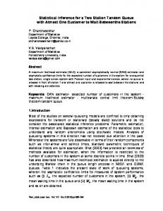
n=50, α=0.26

n=150, α=0.26

n=50

, α=2.5

n=150, α=2.5

Figure 1: Relative probability discrepancy (RPD) versus asymptotic probabilities(γ); With k = 3 Pak.j.stat.oper.res. Vol.XII No.2 2016 pp235-244

241


Figure 1 showed the plots of relative probability discrepancy (RPD) against the asymptotic probability of the asymptotic distribution of quasi t-test based on HC1, HC3, HC4m and HC6. Usually, we are interested in studying the relative probability discrepancy when γ > 0.8. So we will discuss the results specifically for this situation. It can be observed that for sample size when the level of heteroskedasticity is low, HC3 and HC4m have smaller relative probability discrepancy. The situation totally changes when the level of heteroskedasticity is high. The relative probability discrepancy of test based on HC6 decreases in presence of high level heteroskedasticity. While this is the case which adversely affects the asymptotic approximation of HC3 and HC4m. For large sample size, all the three tests, HC3, HC4m and HC6, have shown same amount of relative probability discrepancy especially when γ > 0.7. The behavior of HC1 is generally poor in all the considered scenarios. 5.

Application to Real data

In this section, we apply the quasi t-test for the hypothesis testing of the significance of regression coefficient. The test is applied under the new suggested estimator HC6 and comparison has been made with HC1, HC3, HC4m. The data has been taken from Greene (1997, p.541). This same data set has already been studied in literature see e.g. CribariNeto( 2004), Cribari-Neto et al., (2007) and Cribari-Neto and Zarkos (2004). In this data, the per capita spending on public schools (y) is the response variable while the per capita income of the state (x) is independent variable. The data set consist of 50 observations excluding missing observations. The regression model which is estimated for this data is, Yi   0  1 X 1i   2 X 12i   i , i  1,2,..., 50

(14)

This is the same model studied by Cribari- Neto et al.,(2007). The OLS estimates of the model ˆo  832.9 , ˆ1   1834.2 , ˆ2  1587.0 . The Breusch-pagan test (LM = 18.9035, p.value < 0.001) shows the presence of heteroskedasticity. We wish to test the null hypothesis H0: β2 = 0 against H1: β≠0. Table 2:

Test of heteroskedasticity H0: β2 = 0 Breusch-Pagan test of heteroskedasticity Test Breusch Pagan Testing of H0 : Test OLS HC1 HC3 HC4m HC6

LM d.f 18.903 2 β2 = 0 against H1 : β2 ≠ 0 S.E T 519.1 3.06 856.1 1.85 1995.2 0.8 2553.3 0.62 1146.2 1.38

p-value 0:000 p-value 0.0036 0.0700 0.4303 0.5372 0.1727

From the results given in Table 2 it can be noticed that the test on the OLS standard error rejects the null hypothesis even at 1% level of significance. Same is the case for HC1 242



which rejects the null hypothesis at 10% level of significance. While the test based on other HCCMEs, i.e. HC3, HC4m and HC6, we are unable to reject the null hypothesis even at 10% level of significance. Hence from these results it can be concluded that, the test statistic based on the HC6 estimator will give reliable inference in real life data. 6.

Conclusion

In this article we propose a new HC estimator, called HC6, which used the deviance measure to rescale the residuals. The numerical results suggest that, when the level of heteroskedasticity is very high and sample size is small, the test based on HC6 estimator have better approximation of asymptotic distribution. We recommend using newly suggested estimator instead to other HCCMEs, especially when the sample size is small. We study the estimator only under normal distribution with heteroskedastic disturbances it can also be studied assuming heteroskedasticity under some non normal distribution of the error term. 7.

References

1.

Arce, M. and Mora, A. (2002). Empirical evidence of the effect of European accounting differences on the stock market valuation of earnings and book value. European Accounting Review, 11(3): 573–599.

2.

Chand, S. and Aftab, N. (2012). On finite sample distribution of quasi test statistic based on heteroskedastic consistent covariance matrix estimators. Middle-East Journal of Scientific Research, 12(8): 1157–1164.

3.

Cribari-Neto, F. (2004). Asymptotic inference under heteroskedasticity of unknown form. Computational Statistics & Data Analysis, 45(2): 215–233.

4.

Cribari-Neto, F. and da Silva, W. (2011). A new heteroskedasticity consistent covariance matrix estimator for the linear regression model. AStA Advances in Statistical Analysis, 95(2): 129–146.

5.

Cribari-Neto, F., Souza, T., and Vasconcellos, K. (2007). Inference under heteroskedasticity and leveraged data. Communications in Statistics-Theory and Methods, 36(10): 1877–1888.

6.

Cribari-Neto, F. and Zarkos, S. (1999). Bootstrap methods for heteroskedastic regression models: evidence on estimation and testing. Econometric Reviews, 18(2): 211–228.

7.

Cribari-Neto, F. and Zarkos, S. (2001). Heteroskedasticity consistent covariance matrix estimation: White’s estimator and the bootstrap. Journal of Statistical Computation and Simulation, 68(4): 391–411.

8.

Cribari-Neto, F. and Zarkos, S. G. (2004). Leverage-adjusted heteroskedastic bootstrap methods. Journal of Statistical Computation and Simulation, 74(3): 215–232.

9.

Davidson, R. and MacKinnon, J. (1993). Estimation and inference in econometrics. Oxford University Press, USA.


243


10.

Davidson, R. and MacKinnon, J. (1998). Graphical methods for investigating the size and power of hypothesis tests. The Manchester School, 66(1):1–26.

11.

Eicker, F. (1963). Asymptotic normality and consistency of the least squares estimators for families of linear regressions. The Annals of Mathematical Statistics, 34(2): 447–456.

12.

Greene, W. H. (1997). Econometric analysis. Pearson Education India, 3rd edition.

13.

Hinkley, D. (1977). Jackknifing in unbalanced situations. Technometrics, 19: 285–292.

14.

Horn, S., Horn, R., and Duncan, D. (1975). Estimating heteroskedastic variances in linear models. Journal of the American Statistical Association, 70:380–385.

15.

Long, J. and Ervin, L. (2000). Using heteroskedasticity consistent standard errors in the linear regression model. The American Statistician, 54(3):217–224.

16.

MacKinnon, J. and White, H. (1985). Some heteroskedasticity consistent covariance matrix estimators with improved finite sample properties. Journal of Econometrics, 29(3): 305–325.

17.

Montgomery, D., Peck, E., Vining, G., and Vining, J. (2001). Introduction to linear regression analysis, volume 3.

18.

Wiley New York. R Development Core Team (2011). R: A Language and Environment for Statistical Computing. R Foundation for Statistical Computing, Vienna, Austria.

19.

White, H. (1980). A heteroskedasticity-consistent covariance matrix estimator and a direct test for heteroskedasticity. Econometrica: Journal of the Econometric Society, 48(4): 817–838.

244


Sampling Algorithm of Order Statistics for Conditional ...

Sampling Algorithm of Order Statistics for Conditional ...

Suggest Documents