Sampling Algorithm of Order Statistics for Conditional ...

Variable Control Charts Based on Percentiles of the New Weibull-Pareto Distribution Srinivas Rao Boyapati Department of Mathematics & Humanities R.V.R & J.C College of Engineering Chowdavaram, Guntur- 522 019 Andhra Pradesh, India [email protected]

Suleman Nasiru Department of Statistics, Faculty of Mathematical Sciences University for Development Studies, P.O.Box24, Navrongo Upper East Region, Ghana, West Africa. Ghana [email protected]

K.N.V.R. Lakshmi Department of Statistics, Acharya Nagarjuna University Guntur- 522 010, Andhra Pradesh, India [email protected]

Abstract A variable quality characteristic is assumed to follow the new Weibull- Pareto distribution. Based on the evaluated percentiles of sample statistics like mean, median, midrange, range and standard deviation, the control limits for the respective control charts are developed. The admissibility and power of the control limits are assessed in comparison with those based on the popular Shewhart control limits.

Keywords and phrases: Most probable, Pdf, Cdf, Equi-tailed, Percentiles, NWPD. 1.

Introduction

The well-known Shewhart control charts are developed under the assumption that the quality characteristic follows a normal distribution. If x1, x2,.. xn is a collection of observations of size n on a variable quality characteristic of a product and if tn is a statistic based on this sample, the control limits of Shewhart variable control chart are E(tn)±3S.E(tn). In quality control studies data is always in small samples only. Therefore if the population is not normal there is a need to develop separate procedure for the construction of control limits. In this paper we assume that the quality variate follows the new Weibull-Pareto model and develop control limits for such data on par with the presently available control limits. If a process quality characteristic is assumed to follow the new Weibull-Pareto distribution the online process of such a quality can be controlled through the theory of the new Weibull-Pareto distribution. In the absence of any such specification of the population model we generally use the normal distribution and the associated constants available in all standard text books of statistical quality control. However, normality is only an assumption that is rarely verified and found to be true. Unless the sample is very large in size this assumption may not be taken for granted without proper goodness of fit test procedure. At the same time central limit theorem cannot be made use of, because central limit theorem gives only asymptotic normality for Pak.j.stat.oper.res. Vol.XI No.4 2015 pp631-643

Srinivas Rao Boyapati, Suleman Nasiru, K.N.V.R. Lakshmi

any statistic. Therefore, if a distribution other than normal is a suitable model for a quality variate, separate procedures are to be developed. We present the construction of quality control charts when the process variate is assumed to follow the new WeibullPareto distribution. Let X be a random variable from a Pareto distribution with its cumulative distribution function (cdf) for x ≥ θ given by   F1 ( x;  , k )  1    x

k

(1.1)

where θ >0 is a scale parameter and k>0 is the shape parameter. The probability density function (pdf) corresponding to (1.1) is f1 ( x;  , k ) 

k k

(1.2)

xk 1

The new Weibull-Pareto distribution has a cdf of the form

F ( x)  

1 R( x) 0

f 2 ( x)dx

(1.3)

where R(x) is the survival function of the Pareto distribution and is given by R(x)=1- F1(x; θ, k) while f2(x) is the pdf of a Weibull distribution and is given by f 2 ( x)   (x) 1 e (x)

(1.4)

where x>0, α >0 and λ >0. Using (1.3) and (1.4) given that R(x) =

x k , the cdf of the NWPD is given by

1

F ( x)   ( x )k  (x) 1 e ( x ) dx

(1.5)

F ( x) 1 e  ( x )

(1.6)



0

If we let    and   , then the cdf of the new Weibull-Pareto distribution (NWPD) can be written as

F ( x) 1 e

 ( x ) 

(1.7)

The pdf is given by g ( x) 

  x      

 1

e

 ( x ) 

(1.8)

where 0 < x < ∞, β > 0, θ >0 and δ > 0. The hazard function is given by

  x  h( x )      

632

 1

(1.9)

Pak.j.stat.oper.res. Vol.XI No.4 2015 pp631-643

VARIABLE Control Charts Based on Percentiles of the New Weibull-Pareto Distribution

From the hazard function the following can be observed: (1)

if β = 1, the failure rate is constant, which makes the NWPD suitable for modeling systems or components with failure rate.

(2)

if β > 1, the hazard is an increasing function, which makes the NWPD suitable for modeling components that wears faster with time.

(3)

if β < 1, the hazard is a decreasing function, which makes the NWPD suitable for modeling components that wears slower with time.

The distributional properties are: 1   1 E ( x)        

(1.10)

median =  1 in (2) 

1

(1.11)

1    2       1   2             

2

2

Variance =



(1.12)

The pdf the largest order statistic X(n) is given by n  x   ( n)      

n1

e

 ( x )



 1  e 

 ( x )



 

n1

(1.13)

The pdf of the smallest order statistic X(1) is given by  (1) 

n  x      

n 1

e

 ( x )



  ( x )    e    

n 1

(1.14)

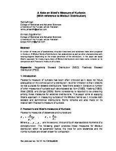
The other distributional properties are thoroughly discussed by Nasiru and Luguterah (2015) [8]. Skewed distributions to develop statistical quality control methods are attempted by many authors. Some of them are Edge-man(1989) [3] – Inverse Gaussion Distribution, Gonzalez and Viles (2000) [4] – Gamma Distribution, Kantam and Sriram(2011) [5]-Gamma Distribution, Chan and Cui (2003) [2] have developed control chart constants for skewed distributions where the constants are dependent on the coefficient of skewness of the distribution, Kantam et al (2006) [6] – Log logistic Distribution, Betul and Yaziki (2006) [1]- Burr Distribution, Subba Rao and Kantam(2008) [11]-Double exponential distribution, Kantam and Rao(2010) [7]-control charts for process variate, Rao and Sarath Babu (2012) [9]-Linear failure rate distribution, Rao and Kantam (2012) [10]-Half logistic distribution and references there in. NWPD is another situation of skewed distribution which is paid much attention with respect to development of control charts in the present study. If β=0.5, δ 1.5 and θ=2.0, then the hazard function indicates a decreasing failure rate function (shown in the graph), which makes the NWPD suitable for modeling components that wears slower with time. At the same time it is one of the probability models applicable for life testing and reliability studies also. Accordingly, if a lifetime data is considered as a quality data, Pak.j.stat.oper.res. Vol.XI No.4 2015 pp631-643

633


development of control charts for the same is desirable for the use by practitioners. Since NWPD is a skewed distribution, this paper makes an attempt to study in a comparative manner. An attempt is made in this paper to address this problem and solve it to the extent possible. The rest of the paper is organized as follows. The basic theory and the development of control charts for the statistics – mean, median, midrange, range and standard deviation are presented in Section 2. The comparative study to the developed control limits in relation to the Shewhart limits is given in Section 3. Summary and conclusions are given in Section 4. Figure 1: Hazard function of the new Weibull-Pareto distribution

2. Control chart constants through percentiles 2.1. Mean-chart. Let x1, x2,..,xn be a random sample of size n supposed to have been drawn from NWPD with β=0.5, δ=1.5 and θ =2.0. If this is considered as a subgroup of an industrial process data with a targeted population average, under repeated sampling the statistic x gives whether the process average is around the targeted mean or not. Statistically speaking, we have to find the ‘most probable’ limits within which x falls. Here the phrase ‘most probable’ is a relative concept which is to be considered in the population sense. As the existing procedures are for normal distribution only, the concept of 3σ limits is taken as the ‘most probable’ limits. It is well known that 3σ limits of normal distribution include 99.73% of probability. Hence, we have to search two limits of the sampling distribution of sample mean in NWPD such that the probability content of those limits is 0.9973. Symbolically we have to find L, U such that P( L  x  U )  0.9973

(2.1)

Where x is the mean of the sample size n. Taking the equi-tailed concept L, U are respectively 0.00135 and 0.99865 percentiles of the sampling distribution of x . We resorted to the empirical sampling distribution of x through simulation there by computing its percentiles. These are given in Table 1. 634



Table 1: Percentiles of Mean in NWPD n

0.99865

0.9950

0.99

0.975

0.95

0.05

0.025

0.01

0.005

0.00135

2

17.4606

10.8759

8.0867

5.1371

3.0376

0.0235

0.0186

0.0151

0.0133

0.0117

3

15.1037

8.7693

6.6472

4.4846

2.9126

0.0318

0.0257

0.0203

0.0174

0.0147

4

11.7977

7.3706

5.7197

3.9353

2.7897

0.0385

0.0323

0.0255

0.0218

0.0182

5

9.7210

6.4674

5.3696

3.6817

2.6375

0.0434

0.0369

0.0308

0.0273

0.0221

6

8.2124

5.8684

4.6866

3.3315

2.4230

0.0480

0.0408

0.0344

0.0302

0.0250

7

7.6891

5.7796

4.3089

3.1712

2.3289

0.0507

0.0441

0.0377

0.0337

0.0277

8

7.1562

5.3255

3.9993

2.9262

2.2647

0.0541

0.0467

0.0402

0.0362

0.0299

9

6.6775

4.7624

3.7982

2.7964

2.1887

0.0578

0.0501

0.0433

0.0389

0.0333

10

6.1537

4.6119

3.6615

2.7455

2.1279

0.0618

0.0537

0.0460

0.0410

0.0350

The percentiles in the above table are used in the following manner to get the control limits for sample mean. From the distribution of x , consider P(Z0.00135 ≤ x ≤ Z0.99865) = 0.9973

(2.2)

But x of sampling distribution when β=0.5, δ=1.5 and θ=2.0 is 1.7777 for NWPD. From equation(2.2) over repeated sampling, for the ith subgroup mean we can have

P( Z 0.00135

x x  x i  Z 0.99865 )  0.9973 1.777 1.777

(2.3)

This can be written as

P( A2 p  x  x i  A2 p x)  0.9973 *

**

(2.4) *

Where x is grand mean, x i is ith subgroup mean, *

A

2p

,

**

A

2p

A

2p

=

Z0.000135 , 1.7777

**

A

2p

=

Z0.99865 , 1.7777

Thus

are the percentile constants of x chart for NWPD are given in Table 2.

Table 2: Percentile constants of Mean-chart n

*

A

9.8217 8.4959 6.6362 5.4681 4.6195 4.3251 4.0254 3.7561 3.4615

0.0066 0.0083 0.0102 0.0124 0.0141 0.0156 0.0168 0.0188 0.0197

2p

2 3 4 5 6 7 8 9 10

**

A


2p

635


2.2. Median-chart We have to search two limits of the sampling distribution of sample median in NWPD such that the probability content of these limits is 0.9973. Symbolically, we have to find L, U such that P(L ≤ m ≤ U) = 0.9973

(2.5)

Where m is the median of sample size n. Through simulation, the percentiles observed are given in Table 3. Table 3: Percentiles of Median in NWPD n

0.99865

0.9950

0.99

0.975

0.95

0.05

0.025

0.01

0.005

0.00135

2

17.4606

10.8759

8.0867

5.1371

3.0376

0.0235

0.0186

0.0151

0.0133

0.0117

3

5.9335

4.0277

2.6446

1.4857

0.7665

0.0203

0.0164

0.0140

0.0127

0.0114

4

4.5757

2.8170

2.1675

1.3434

0.7944

0.0277

0.0223

0.0184

0.0162

0.0141

5

3.1791

1.7332

1.2423

0.6366

0.2653

0.0255

0.0212

0.0173

0.0155

0.135

6

2.0708

1.3295

0.9849

0.6082

0.3367

0.0311

0.0261

0.0218

0.0191

0.0154

7

1.5430

1.0200

0.7286

0.3027

0.1399

0.0290

0.0243

0.0203

0.0180

0.0157

8

1.3092

0.8493

0.6391

0.3668

0.1927

0.0333

0.0284

0.0240

0.0208

0.0173

9

1.0695

0.6782

0.4413

0.1980

0.1336

0.0322

0.0274

0.0234

0.0207

0.0179

10

1.0399

0.5928

0.4215

0.2016

0.1340

0.0351

0.0306

0.0262

0.0235

0.0201

The percentiles in the above table are used in the following manner to get the control limits for median. From the distribution of m, consider

PZ 0.00135  m  Z 0.99865  0.9973

(2.6)

But median of sampling distribution when β=0.5, δ=1.5, and θ=2.0 is 0.42707 for NWPD. From equation (2.6) over repeated sampling, for the ith subgroup median we can have P( Z 0.00135

m m  mi  Z 0.99865 ) 0.42707 0.42707

(2.7)


P( A7 p m  mi  *

**

A

7p

m)  0.9973

(2.8)

Z 0.00135 Z ** , A7 p  0.99865 are the 0.42707 0.42707 percentile constants of median chart and are given in Table 4. *



where m is mean of subgroup medians. Thus

A

636


7p


Table 4: Percentile constants of Median-chart n

*

**

A

A

40.8847 13.8935 10.7141 7.4439 4.8487 3.6130 3.0656 2.5044 2.4349

0.0273 0.0268 0.0329 0.0317 0.0362 0.0367 0.0404 0.0419 0.0470

2p

2 3 4 5 6 7 8 9 10

2p

2.3 Midrange-chart. We have to search two limits of the sampling distribution of sample midrange in NWPD such that the probability content of these limits is 0.9973. Symbolically, we have to find L, U such that P(L ≤ M ≤ U) = 0.9973

(2.9)

where M is the midrange of sample size n. Through simulation, the percentiles observed are given in Table 5. Table 5: Percentiles of Midrange in NWPD n

0.99865

0.9950

0.99

0.975

0.95

0.05

0.025

0.01

0.005

0.00135

2

17.4606

10.8759

8.0867

5.1371

3.0376

0.0235

0.0186

0.0151

0.0133

0.0117

3

22.6093

12.4842

9.5671

6.2095

3.9511

0.0327

0.0268

0.0208

0.0179

0.0184

4

22.6993

13.5701

10.5881

7.0163

4.7670

0.0415

0.0346

0.0274

0.0232

0.0184

5

23.4614

15.0277

11.6465

7.9251

5.4832

0.0499

0.0417

0.0343

0.0297

0.0235

6

23.4643

15.1905

12.3891

8.6729

6.0953

0.0566

0.0485

0.0393

0.0345

0.0290

7

23.4790

17.1724

12.5901

9.2402

6.6306

0.0609

0.0532

0.0447

0.0393

0.0320

8

24.4671

18.0809

13.4355

9.5140

6.9891

0.0640

0.0566

0.0488

0.0433

0.0354

9

25.6823

18.8002

14.0853

10.0124

7.4294

0.0690

0.0613

0.0532

0.0475

0.0381

10

27.2125

19.6400

15.0062

10.8240

7.9756

0.0731

0.0659

0.0587

0.0547

0.0460

The percentiles from the above table are used in the following manner to get the control limits for midrange. From the distribution of M, consider P(Z0.00135 ≤ M ≤ Z0.099865) = 0.9973

(2.10)

The midrange value of NWPD is calculated by using α(1) and α(n).


637


From equation (2.10) for ith subgroup midrange we can have, P( Z 0.00135

M M  M i  Z 0.99865 )  (1)   ( n )  (1)   (n) 2 2

(2.11)


P( A4 p M  M i  A4 p M )  0.9973 *

**

(2.12)

2Z 0.0135 2Z 0.99865 ** , A4 p  are the  (1)   ( n )  (1)   ( n ) percentile constants of midrange chart for NWPD process data given in Table 6. where M is mean of midranges. Thus

*

A

4p



Table 6: Percentile constants of Midrange-chart n

*

**

A

A

831.6948 74.6447 18.9612 12.6372 8.4244 6.3816 5.4154 4.2019 2.9148

0.0025 0.0027 0.0028 0.0035 0.0048 0.0057 0.0059 0.0066 0.0069

2p

2 3 4 5 6 7 8 9 10

2p

2.4 R-Chart. We have to search two limits of the sampling distribution of sample range in NWPD such that the probability content of these limits is 0.9973. Symbolically, we have to find L, U such that P(L ≤ R ≤ U) = 0.9973 (2.13) where R is the range of sample of size n. Through simulation, the percentiles observed are given in Table 7. Table 7: Percentiles of Range in NWPD n

0.99865

0.9950

0.99

0.975

0.95

0.05

0.025

0.01

0.005

0.00135

2

34.2650

20.8141

14.4759

9.0737

5.5478

0.0049

0.0025

0.0011

0.0006

0.0002

3

45.1667

24.7559

18.9930

12.2815

7.7970

0.0230

0.0152

0.0095

0.0062

0.0031

4

45.1837

27.0879

21.1320

13.9184

9.4607

0.0424

0.0313

0.0209

0.0168

0.0085

5

46.8067

29.9866

23.2380

15.8182

10.8957

0.0608

0.0467

0.0341

0.0270

0.0180

6

46.8871

30.3313

24.7370

17.3004

12.1545

0.0747

0.0616

0.0466

0.0387

0.0293

7

46.8951

34.3161

25.1334

18.4278

13.2014

0.0867

0.0745

0.0580

0.0488

0.0345

8

48.9082

36.1374

26.8441

18.9777

13.9462

0.0963

0.0801

0.0674

0.0567

0.0426

9

51.3310

37.5642

28.1267

19.9926

14.8265

0.1066

0.0904

0.0750

0.0663

0.0494

10

54.3942

39.2441

29.9866

21.6165

15.9104

0.1145

0.1021

0.0888

0.0787

0.0644

638



The percentiles from the above table are used in the following manner to get the control limits for sample range. From distribution of R, consider P(Z0.00135 ≤ R ≤ Z0.99865) = 0.9973 (2.14) From equation (2.14), for the 1th subgroup range we can have R R (2.15) P( Z 0.00135  Ri  Z 0.99865 )  0.9973  ( n )   (1)  ( n)   (1) This can be written as

P( D3 p R  Ri  D4 p R)  0.9973 *

**

(2.16)

Thus R is mean of ranges, Ri is ith subgroup range. Z 0.00135 Z 0.99865 * ** D3 p   (n)   (1) , D4 p   (n)   (1) are the percentile constants or R chart for NWPD process data and are given in Table 8. where

Table 8: Percentile constants of Range-chart n

*

**

A

A

980.4490 136.4872 18.4992 12.6301 8.7324 6.1692 5.2819 4.3546 3.1214

0.0001 0.0005 0.0009 0.0017 0.0037 0.0048 0.0052 0.0054 0.0065

2p

2 3 4 5 6 7 8 9 10

2p

2.5. σ – chart. We have to search two limits of the sampling distribution of sample standard deviation in NWPD such that the probability content of these limits is 0.9973. Symbolically, we have to find L, U such that P(L ≤ s ≤ U) = 0.9973 (2.17) where is the standard deviation of sample of size n. Through simulation the percentiles observed are given in Table 9. Table 9: Percentiles of Standard deviation in NWPD n 2 3 4 5 6 7 8 9 10

0.99865 17.1325 21.2813 19.5441 18.2745 17.4450 16.4010 16.0333 15.9565 16.0461

0.9950 10.4071 11.5345 11.6939 11.9902 11.2582 11.8551 12.0707 11.9852 11.9484

0.99 7.2380 8.8545 8.9431 9.1641 9.0273 8.8169 8.8157 8.8994 9.0755

0.975 4.5368 5.6890 5.9253 6.3103 6.3984 6.4205 6.2189 6.2719 6.4586


0.95 2.7739 3.6081 4.0238 4.3426 4.4944 4.5818 4.6598 4.7164 4.8295

0.05 0.0024 0.0097 0.0165 0.0224 0.0262 0.0301 0.0323 0.0349 0.0377

0.025 0.0013 0.0066 0.0122 0.0173 0.0215 0.0254 0.0273 0.0298 0.0326

0.01 0.0005 0.0041 0.0083 0.0128 0.0163 0.0199 0.0221 0.0249 0.0282

0.005 0.0003 0.0027 0.0064 0.0097 0.0140 0.0168 0.0193 0.0221 0.0255

0.00135 0.0001 0.0013 0.0033 0.0066 0.0107 0.0121 0.0137 0.0169 0.0213 639


The percentiles from the above table are used in the following manner to get the control limits for sample standard deviation. From distribution of s, consider P(Z0.00135 ≤ s ≤ Z0.99865) = 0.9973

(2.18)

But standard deviation of sampling distribution when β=0.5, δ=1.5 and θ=2.0 is 3.9752 for NWPD. From equation (2.18), for the 1th subgroup standard deviation we can have P( Z 0.00135

S S  Si  Z 0.99865 )  0.9973 3.9752 3.9752

(2.19)


P( B3 p S  Si  B4 p S )  0.9973 *

**

(2.20)

where S is mean of standard deviation, si is ith subgroup standard deviation. Thus Z .00135 ** Z 0.99865 * are the constants of standard deviation chart for NWPD , B4 p  B3 p  3.09752 3.9752 process data given in Table 10. Table 10: Percentile constants of SD-chart n

*

A

4.3098 5.3535 4.9165 4.5971 4.3885 4.1258 4.0333 4.0140 4.0365

0.0001 0.0003 0.0008 0.0017 0.0027 0.0030 0.0034 0.0042 0.0054

2p

2 3 4 5 6 7 8 9 10

**

A

2p

3. Comparative study The control chart constants for the statistics mean, median, midrange, range and standard deviation developed in section 2 are based on the population described by NWPD. In order to use this for a data, the data is confirmed to follow NWPD. Therefore the power of the control limits can be assessed through their application for a true NWPD data in relation to the application for Shewhart limits. With this back drop we have made this comparative study simulating random samples of size n=2,…,10 from NWPD and calculated the control limits using the constants of section 2 for mean, median, midrange, range and standard deviation in succession. The number of statistic values that have fallen within the respective control limits is evaluated and is named as NWPD coverage probability. Similar count for control limits using Shewhart constants available in quality control manuals are also calculated. These are named as Shewhart coverage probability. The coverage probabilities under the two schemes namely true NWPD, Shewhart limits are presented in the following Tables 11, 12, 13, 14 and 15. 640



Table 11: Coverage Probabilities of Mean-chart n 2 3 4 5 6 7 8 9 10

Shewhart limits Coverage x  A2 R x  A2 R probability 0 2.672798 0.9402 0 2.34902 0.9328 0 2.165413 0.9290 0 2.103061 0.9266 0 2.056731 0.9284 0 2.039132 0.9344 0 2.028127 0.9384 0 2.016057 0.9400 0 1.416339 0.9414

Percentile limits *

A

2p

x

0.004188 0.005363 0.006474 0.007906 0.008951 0.00997 0.010778 0.012076 0.012758

**

A

2p

x

6.231820 5.489357 4.212125 3.486211 2.932608 2.764115 2.582339 2.412671 2.241706

Coverage probability 0.9831 0.9831 0.9772 0.9718 0.9651 0.9656 0.7509 0.9618 0.9558

Table 12: Coverage Probabilities of Median-chart n 2 3 4 5 6 7 8 9 10

Shewhart limits Coverage m  A7 R m  A7 R probability 0 2.672798 0.9402 0 1.964569 0.9839 0 1.860031 0.9857 0 1.793225 0.9955 0 1.821971 0.9982 0 1.833368 0.9994 0 1.867169 0.9997 0 1.893424 1.0000 0 1.943247 0.9999

Percentile limits *

A

7p

m

0.017322 0.005050 0.006207 0.003706 0.004146 0.003395 0.003796 0.003500 0.003954

**

A

7p

m

25.94167 2.61798 2.021397 0.870356 0.555331 0.334203 0.288032 0.209200 0.204838


Table 13: Coverage Probabilities of Midrange-chart n 2 3 4 5 6 7 8 9 10

M  A4 R

0 0 0 0 0 0 0.231055 0.344156 0.589542

Shewhart limits Coverage M  A4 R probability 3.044678 1.0000 2.98237 0.9666 2.819352 0.9750 3.104208 0.9600 3.152125 0.9333 3.432268 0.9429 3.524695 0.1125 3.768274 0.1340 3.881828 0.0800


Percentile limits *

A

4p

M

0.001586 0.002362 0.003026 0.004535 0.007175 0.009641 0.011079 0.013571 0.015426

**

A

4p

M

527.717 65.31232 20.49321 16.3757 12.59221 10.79384 10.16944 8.64001 6.516575

Coverage probability 1.0000 1.0000 1.0000 1.0000 1.0000 1.0000 0.9625 0.9559 0.8800 641


Table 14: Coverage Probabilities of Range-chart n 2 3 4 5 6 7 8 9 10

D3 R

0 0 0 0 0 0.253946 0.505566 0.750039 0.989451

Shewhart limits Coverage D4 R probability 3.542081 0.9177 4.286345 0.8923 4.791515 0.8776 5.371677 0.8667 5.908994 0.8568 6.428854 0.6263 6.929234 0.5911 7.402561 0.5672 7.884549 0.5504

Percentile limits *

D

3p

R

**

D

4p

0 0.000832 0.00189 0.004318 0.01091 0.016039 0.01933 0.022012 0.028841

R

1063.003 227.1966 38.84277 32.07793 25.74835 20.61376 19.63494 17.75066 13.84965


Table 15: Coverage Probabilities of SD-chart n 2 3 4 5 6 7 8 9 10

Shewhart limits Coverage B3 S B4 S probability 0 1.771034 0.9177 0 1.962165 0.8923 0 2.013366 0.8469 0 2.090730 0.8636 0.03267 2.145344 0.7572 0.137953 2.200231 0.5632 0.229226 2.248894 0.5359 0.310508 2.287884 0.5113 0.386105 2.332943 0.4925

Percentile limits *

B

3p

S

0 0.000229225 0.000710809 0.001701408 0.002940319 0.003507276 0.004212804 0.005456623 0.00734143

**

B

4p

S

2.336334 4.090518 4.368364 4.600906 4.779107 4.823440 4.997501 5.214973 5.487719


4. Summary & Conclusions The Tables 11, 12, 13, 14 and 15 show that for a true NWPD if the Shewhart limits are used in a mechanical way it would result in less confidence coefficient about the decision of process variation for mean, median, midrange, range and standard deviation charts. Hence if a data is confirmed to follow NWPD, the usage of Shewhart constants in all the above charts is not advisable and exclusive evaluation and application of NWPD constants is preferable in statistical quality control. Acknowledgments The authors thank the Editor and the reviewers for their helpful suggestions, comments and encouragement, which helped in improving the final version of the paper. References 1.

642

Betul kan and Berna Yaziki The Individual Control Charts for BURR distributed data In proceedings of the ninth WSEAS International Conference on Applied Mathematics, Istanbul, Trukey, pages 645-649, 2006. Pak.j.stat.oper.res. Vol.XI No.4 2015 pp631-643


2.

Chan. Lai. K., and Heng. J. Cui Skewness Correction x and R-charts for skewed distributions Naval Research Logistics, 50:1-19, 2003.

3.

Edgeman. R.L Inverse Gaussian control charts Australian Journal of Statistics, 31(1):435-446, 1989

4.

Gonzalez. I., and Viles. I., Semi-Economic design of Mean control charts assuming Gamma Distribution Economic Quality Control, 15:109-118, 2000.

5.

Kantam. R.R.L., and Sriram. B., Variable control charts based on Gamma distribution IAPQR Transactions, 26(2): 63-67, 2001.

6.

Kantam R.R.L., Vasudeva Rao. A., and Srinivasa Rao. G., Control Charts for Log-logistic Distribution Economic Quality Control, 21(1):77-86, 2006.

7.

Kantam. R.R.L., and Srinivasa Rao. B., An improved dispersion control charts for process variate International journal of Mathematics and Applied Statistics, 1(1): 19-24, 2010.

8.

Nasiru. S., and Luguterah. A., The new Weibull-Pareto distribution Pakistan Journal of Statistics and Operations Research, 11(1):103-114, 2015.

9.

Srinivasa Rao B., and Sarath babu. G., Variable control Charts based on Linear Failure Rate Model International Joural of Statistics and Systems, 7(3):331-341, 2012.

10.

Srinivasa Rao B., and Kantam. R.R.L., Mean and range charts for skewed distributions – A comparison based on half logistic distribution Pakistan Journal of Statistics, 28(4):437-444, 2012.

11.

Subba Rao. R., and Kantam. R.R.L., Variable control charts for process mean with reference to double exponential distribution Acta Cinica Indica, 34(4): 1925-1930, 2008.


643

Sampling Algorithm of Order Statistics for Conditional ...

Sampling Algorithm of Order Statistics for Conditional ...

Suggest Documents