Sampling Algorithm of Order Statistics for Conditional ...

Structural Breaks, Automatic Model Selection and Forecasting Wheat and Rice Prices for Pakistan Zahid Asghar Quaid-i-Azam University,Islamabad, Pakistan. [email protected]

Amena Urooj PIDE, Islamabad, Pakistan [email protected]

Abstract Structural breaks and existence of outliers in time series variables results in misleading forecasts. We forecast wheat and rice prices by capturing the exogenous breaks and outliers using Automatic modeling. The procedure identifies the outliers as the observations with large residuals. The suggested model is compared on the basis of Root Mean Square Error (RMSE) and Mean Absolute Percentage Error (MAPE) with the usual ARIMA model selected ignoring the possible breaks. Our results strongly support that forecasting with breaks by using General to Specific (Gets through Autometric) model performs better in forecasting than that of traditional model. We have used wheat and rice price data (two main staple foods) for Pakistan.

Key words: General-to-specific (gets) Modeling, Structural Breaks, Impulse Saturation Regression Modeling, Wheat Inflation Rate, Rice Inflation Rate, 12-Step Forecast, Automatic Model Selection, RMSE, MAPE.

1.

Introduction:

In the continuously changing scenario of the global economy, policy making is the major issue related to the growth and development of an economy. Effective policy making requires continuous follow up of behavior and trends of macroeconomic variables, for which time series data is used. In making strategic decisions under uncertainty, time series forecasting is the major tool applied at all levels. In practice, an effective approach to time-critical dynamic decision modeling should provide explicit support for the modeling of temporal processes and for dealing with time-critical situations. Thus among the major goals of time series data forecasting for policy making is the most important. And it requires effective and accurate modeling of time series data. However, time series data are hard to handle and require complicated statistical and econometrics based procedures to model. In order to match theory and evidence, researchers are forced to adopt some form of model selection procedure. Although there exist several approaches each having some properties but each of those face criticism as well. In general the model selection criteria inquire the satisfactory answer of several queries like if the diagnostic tests are satisfactory? Are all important variables included in the model? Are some superfluous variables included? Is the functional form of the chosen model correct? Is the specification of the stochastic errors correct? Is there more than one specification error?

Pak.j.stat.oper.res. Vol.VIII No.1 2012 pp1-20

Zahid Asghar, Amena Urooj

The traditional view of model selection in econometrics is: The Average Economics Regression (AER) or Bottom Up approach, under which the basic model is selected (initiated) with a given number of regressors, based upon some economic theory. Then, based upon the model diagnostics, more variables are added or subtracted to build the appropriate model. However, according to Gilbert (1986), the main problem with the AER approach is that it uses econometrics to illustrate independently held a priori theories. The AER approach, according to Darnell & Evans (1990), becomes a data-mining exercise where the data is thrashed until it eventually reveals a model with the pleasing characteristics described under some theory. Moreover, it is an arbitrary approach and may lead to different (varied) results. General-to-specific (gets) modeling has been developed and applied through computer automated form in the Pc Gets software (Hendry and Krolzig2001). The idea is to specify a congruent general unrestricted model (GUM) that captures the main features of the data generation process (DGP) or local DGP sufficiently well so that it is not rejected by the data in a range of specification tests. Then statistical tests and procedures are used to reduce the model as much as possible to obtain a congruent more parsimonious model for the (local) DGP of the time series under investigation. Forecasts of economic variables play a prominent role in business decision making, government policy analysis, and economic research. Forecasts often are model-based, with forecasts from an estimated model being constructed as the model‘s fitted values over a sample that was not used in estimation. Sources of forecast error depend on the forecast model itself and on the process generating the data. Clements and Hendry (1999) state that economics forecasts are sometimes terribly wrong due to the existence of structural breaks in data. When economic systems are subject to structural breaks, conventional models need not forecast satisfactori1y. Previously unannounced changes in policy, natural and man-made disasters, institutional changes, new discoveries, new data definitions and revisions among others cause occasional large forecast errors in the standard constant parameter model. The existence of outliers and structural breaks in the model badly affect the identification, estimation and inference of the model. It causes the confidence interval of the coefficient to be dramatically increased as well and results in misleading forecasts. Stock and Watson (1996, 1999) show that instability pervades a wide range of time series due to structural breaks causing failure of forecast. The historical evidence of recurrent episodes of the economic forecasting failure has forced the researchers to develop such methods which avoid these mistakes. Amongst several proposed techniques is the impulse saturated modeling, the intercept correction and double differencing in vector equilibrium correction models (VECMs). The objective of this study is to forecast wheat and rice price at retail level by using an ARIMA model. We shall examine the impact of structural breaks through impulse saturated regression using automatic model selection on the forecast of two major macro-economic variables of Pakistan. Motivation behind forecasting these two variables is their importance in food share of Pakistani population. Wheat share in our food in 2


Structural Breaks, Automatic Model Selection and Forecasting Wheat and Rice Prices for Pakistan

terms of calories is about 40-55% depending upon income groups and rice share is about 10%. Any increase in price of these two staple foods has very serious repercussions for Pakistani population in general and poor in particular. Therefore, it is important to have an accurate forecast of these variables. For monthly growth rate of wheat prices, retail wheat prices series for monthly time sequence over January 2004 to April 2011 has been used and for monthly growth rate of rice prices, retail basmati rice prices series for monthly time sequence over January 2006 to February 2011 has been considered. We have collected this data from Federal Bureau of Statistics. The study proceeds as follows. Section 2 provides an overview of forecast in presence of structural breaks and its consequences. Section 3 discusses the development of impulse saturated modeling technique. Section 4 and 5 contains the empirical results and discussion. Section6 gives conclusion. 2.

Forecasting In The Presence Of Structural Breaks:

Forecasts typically differ from the realized outcomes, with discrepancies between forecasts and outcomes reflecting forecast uncertainty. Ericsson (2008) stated that the forecast models typically have three components: the variables of the model, the coefficients of those variables, and unobserved errors or shocks. Each component can contribute both predictable and unpredictable uncertainty to the forecast although, in practice, the uncertainty in the measurement of the variables themselves is typically treated as being entirely unpredictable. 1.

Sources of predictable uncertainty (a) Accumulation of future errors (―shocks‖) to the economy (b) Inaccuracies in estimates of the forecast model‘s parameters 2. Sources of unpredictable uncertainty (a) Currently unknown future changes in the economy‘s structure (b) Miss-specification of the forecast model (c) Miss-measurement of the base-period data. An econometric theory of economic forecasting will only deliver relevant conclusions about empirical forecasting if it adequately captures the appropriate aspects of the real world to be forecasted. Fildes and Makridakis (1995) suggest that the most serious culprit is the assumption of constancy which underpins that paradigm. The historical evidence of recurrent episodes of the economic forecasting failure has forced to develop such methods which avoid these mistakes. The complicated system of economies is attempted to be presented through a model which may/may not be the true representative. Then it is a fact that economies are prone to several unanticipated political, economic, social, scientific and natural shifts. If the economic model identified as representative does not incorporative these changes then it will surely has the adverse effect on forecast. Clements and Hendry (1998) have suggested a need to reappraise the modeling approaches to get improved results of macroeconomics forecasting in the presence of structural breaks. Focusing on system of co integrated relation when economies are subjected to unanticipated large regime shifts, the authors have analyzed rigorously the impact of the structural breaks on systematic forecast error stating with the first order autoregressive process with a break in Pak.j.stat.oper.res. Vol.VIII No.1 2012 pp1-20

3


mean the authors consider a variety of models (ARIMA). In connection to this idea, Clements and Hendry (2002) identify that the existence of such location shifts which change the underlying equilibrium mean of the co integration relationship that are not modeled leads to failure. However shifts in other parameters are difficult to detect. Hendry and Doornik (1997) and Hendry (2000) have showed that location shifts are most pernicious problem for forecasting even causing forecasting failure. Clements and Hendry (1998, 1999) have showed that an economic theory providing causal basis for forecasting models is of no avail in a world of location shifts. The idea that large outliers signal the shift to a new equilibrium rather than a large deviation from the current is modeled in a paper by Engle and Smith (1998). Hendry (2004) has considered a first order VAR model as a co integrated DGP and specified its properties as a forecasting device. He has considered the effects of location shift that leads up to a massive forecast failure. Then suggested two approaches in form of using double differencing and the elimination of equilibrium mean. It was later on identified that the second differenced forecasting devices may perform well finally an empirical example of the behavior of MI in UK is discussed in the detail in relation to the above suggested scenario. Haywood and Randal (2007) provides a good account on the poor performance of the existing econometric methods for endogenously dating multiple structural breaks especially with seasonal data. They suggest an iterative nonparametric estimation method based on Bai and Perron (1998, 2003) for estimating the parametric structural breaks. Using the monthly data of tourist arrived in New Zealand, they focus to detect any long term, or result of 9-11 events and compare it with other historical events. Pearson and Timmermann (2004) have suggested a theoretical framework for the analysis of small sample properties of forecasts from general autoregressive models under structural breaks. They have considered for the possibility of the AR model to switch from a unit root process to a stationary one and vice versa. They have also established that one-step ahead forecast errors from AR models are unconditionally unbiased even in the presence of breaks in the autoregressive coefficients and in the error variances so long as the unconditional mean of the process remains unchanged. They present extensive numerical results quantifying the effect of the sizes of the pre-break and postbreak data windows on parameter bias and RMSFE. Moreover undertake an empirical analysis for a range of macroeconomic time series from the G7 countries that compares the forecasting performance of expanding window, rolling window and post-break estimators. This analysis which allows for multiple breaks at unknown times confirms that, at least for macroeconomic time series such as those considered there, it is generally best to use pre-break data in estimation of the forecasting model. Clements and Hendry (2008) summarize the key result that intercept correction places the model back on track at the forecast origin, setting the most recent ex post forecast error to zero. They have suggested a procedure that offsets deterministic shifts after they have occurred. Intercept correction should typically be implemented if shifts are suspected, as when forecast failure has recently 4



occurred. The authors have highlighted that when using the equilibrium correction model (ECMs) the problem faced was that it still converged to their built in equilibrium and hence caused far reaching adverse effect even leading to forecasting failure. They have compared the theory of shifts to the fat tailed distribution, where shocks might occur more frequently. Later on, observing several factors leading to forecast failure it has been argued that parameter inconsistency is the biggest trouble of them all. Finally methods including intercept correlation and forecast combination are discussed to circumvent the forecast failure. The discussion is supplemented with the empirical analysis. They have identified that the models that inherently preclude deterministic terms can never suffer from deterministic shifts, so these models are unlikely to experience systematic forecast failure. Reformulating econometric models to make them more robust to such shifts becomes a priority. A potential solution is intercept correction, which adjusts an equation‘s constant term when forecasting. Clements and Hendry (2008) suggested using a single model differently in those different contexts–for instance, by modeling the data with an equilibrium correction model (ECM) but forecasting from a differenced. Ericsson (2008) has discussed the Clements and Hendry (2008) article by examining the determinants of forecasting uncertainty. Partitioning the source of forecast error in to predictable and unpredictable author discussed the Clements and Hendry‘s taxonomy and its effect. It has been identified that the currently unknown future change is the most fatal source of variation in the forecasts. The Mean Square Forecast Error (MSFE), as a criterion for evaluating forecasting has been criticized using empirical evidence as it lacks the robustness. Castle, et.al (2008) has highlighted the problem in forecasting due to the occurrence of breaks especially location shifts faced by the equilibrium correlation model based on cointegration. Bayesian forecasting methods are less frequently used despite their apparent success both in univariate forecast competitions and in vector auto regression environments.(See e.g. West and Harrison, 1989). Recognizing the importance of density forecasts, rather than simple point forecasts, the Bayesian approach has clear advantages in terms of delivering posterior odds distributions—even across unit root regions of the parameter space. 3.

Impulse saturation Modeling:

The General-to-specific (gets) modeling approach has been applied mainly for single equation time series modeling. Impulse saturation (Hendry, Johansen and Santos, 2007) is a major recent development in model selection. It entails the possibility of testing an individual impulse indicator for each observation in a sample. Groups of indicators are entered in the econometric model in feasible subsets of halves (T/2), thirds (T/3) or any other even or uneven sample partition. Subset selection is then used to retain the relevant indicators from each terminal model into a union model. The indicator variables observe and study the variation (deviations) caused to the economic variables. In static model, adding an indicator is equivalent adjusting the degree of freedom appropriately. However, in dynamic models, indicator variables play a complicated role especially when other regressors play significant role.


5


The power properties of impulse saturation algorithm applied to any model refers to its ability of detecting additive and level shifts at unknown data. The authors have derived the asymptotic distribution of the sample mean and the sample variance in a impulse location-scale model with i.i.d. observations, after saturation. Monte Carlo evidence has shown that under the null hypothesis of no indicator is in the DGP, the average retention rate matches the binomial result , showing no signs of spurious retention. Furthermore, the number of sample splits is also shown to be irrelevant, under the null, for the number of indicators retained. Santos and Hendry (2006), and Nielsen and Johansen (2007) has shown that the procedure can be extended to certain classes of dynamic models. Santos (2008) has evaluated impulse saturation as a test for multiple breaks with unknown locations, and concluded that the procedure has good power properties both against mean and variance shifts. Hendry and Santos (2007) extended this idea to develop a new class of automatically computable super exogeneity tests (see, inter alia, Engle, Hendry and Richard (1983) and Engle and Hendry (1993)). 4.

Empirical Analysis of Wheat price inflation and Rice Price inflation:

Pakistan has been observing a continuous surge in food prices since 2008 when oil prices jumped to almost 150 US dollar a barrel. Normally, prices are expected to fall slightly above their previous level, but unfortunately in case of Pakistan, this didn‘t happen and food prices exhibited an upward trend. These very high prices are causing a reduction in food consumption for most of the Pakistani population. The poorest are the highest to suffer from high food prices. Government also has to utilize more foreign reserves to import food items like edible oil, sugar etc. Donor agencies also face the burden of high food prices to provide assistance to the poor. 4.1

Analysis of the monthly Wheat Prices (Rs. / kg) and forecasting through ARIMA modeling

Graphical examination of the data is important. Series should be examined in levels, logs, differences and seasonal differences. The series should be plotted against time to assess whether any structural breaks, outliers or data errors occur. If so, one may need to consider use of intervention or dummy variables. For monthly growth rate of wheat prices, retail wheat prices series for monthly time sequence over January 2004 to April 2011 has been considered here. Data were collected from Federal Bureau of Statistics and the choice for time period is matched with Food and Agriculture Organization (FAO) time periods. FAO uses this data range to display country price situation. We consider the percentage "annualized" change in the monthly series in order to observe the growth rate. The graphical analysis of wheat inflation indicates the possible existence of unit root or structural break in the data that has to be checked. Plotting the correlogram (useful aid for determining the stationarity of a time series, and an important input into Box-Jenkins model identification). The maximum lag length considered is usually no more than n/4, where n is the total number of observation in a time series. If a time series is stationary then its correlogram

6



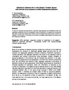
should decay quite rapidly from its initial value of unity at zero lag. If the time series is non-stationary then the correlogram will only die out gradually over time. Figure (1):

Historigram of wheat prices for monthly time series over January 2004 to April 2011

Unit root results are displayed in Table 1 with lag length in parenthesis. We have selected lag length based on standard criteria AIC and SIC. Table (1):

Summary of Results of the Test for the Existence of Unit root in Wheat Inflation Rate.

Y(w)= Wheat Inflation Rate (Δ12ln(wheat prices)) Test for existence of Unit root Calculated value of test statistics Remarks ADF -2.981279(0) Reject H0 PP -2.891070(3 band width) Reject H0 KPSS 0.298602(6 band width) Do not Reject H0 For the model identification several plausible modification of ARIMA (p, d, q)(P,D,Q)12 models with the lags in seasonal and non-seasonal parts varying from 0 to 12 (non-seasonal) and 0 to 1 for seasonal part are examined. The decision between the various possibilities for SARIMA structure is primarily based on finding the minimum value for the Akaike Information Criteria (AIC) and Bayesian information criteria of Schwartz (SIC). After checking all plausible models the finally selected SARIMA Model for the monthly wheat inflation series over the period of 2004:1-2011:4 is (1,0,0)(0,0,0)12 with the minimum AIC of 7.12749, and SIC equals to 7.19495. The above model passes all diagnostic tests namely the AR test (1-4 lags), the ARCH (1-4 lags) test, the Normality test etc.The model is: ( )

( )

(

)(

)(

)

(4.1)

The summary statistics of the model for the estimation sample of 2005(5) 2010(10) along with the 1-step (ex post) forecast analysis 2010(11) - 2011(4) is given in Table 2. Pak.j.stat.oper.res. Vol.VIII No.1 2012 pp1-20

7


Table (2): Summary Statistics for Wheat Inflation Rate ( ) Table (2-a):The Summary Statistics Coefficient Std. Error t-value ( ) 0.765238 0.08138 9.4 Constant 3.21963 1.565 2.06 Diagnostic Analysis RSS R^2 4511.36484 0.580136

t-prob 0 0.0438

Part.R^2 0.5801 0.062 1.83

log-likelihood

-233.065

FPE

1240.42

AIC AR 1-5 test: F(5,59) Hetero test: F(2,61) mean(Y)

7.12318 0.80064 [0.5537] 0.44467 [0.6431] 14.2765

SC ARCH 1-5 test: (5,54) no. of parameters Var (Y)

7.18954 1.1500 [0.3457]

DW no. of observations HQ RESET test: F(1,61)

2

F(1,63) =

66 7.1494 3.0472 [0.0858] 88.43 [0.000]**

162.8

Table (2-b): 1-step (ex post) forecast analysis 2010(11) - 2011(4) Parameter constancy forecast tests: Forecast Chi^2(6) MAPE 0.79861 [0.9921] 179.04 Chow F(6,64) RMSE 0.11703 [0.9941] 3.0631 CUSUM: t(5) -0.7596 [0.4817] (zero forecast innovation mean)

Figure(2) gives the plot of the actual and the fitted monthly wheat inflation rates. Figure (2): Actual and Fitted Monthly Wheat Inflation Rates.

The forecasting method here is based on simulation for later months from the earlier ones assuming zero shocks over the forecasting horizon. The forecast for the following 12 months from this estimation is obtained for the horizon h=1, 3, 6, and 12. Thus any structural or regime change in the series during the fourth coming time period is not taken into account. The second panel of table (2) shows the root mean squared errors (RMSE) and the Parameter constancy forecast tests. Figure (3 a, b, c, d) shows the forecast and the actual inflation from the automatic regression modeling over four different forecasting horizons.

8



Figure (3): Automatic Regression Modeling for Four Forecasting Horizons. (b) h = 3 (a) h = 1

(c) h = 6

(d) h=12

Table (3):12-step forecast for Wheat Inflation Rate ( ) Horizon Forecast SE Actual Error 2010-11 6.49218 8.396 4.27651 -2.21566 2010-12 8.18769 10.57 4.27651 -3.91117 2011-1 9.48516 11.66 1.42811 -8.05705 2011-2 10.478 12.25 1.08623 -9.3918 2011-3 11.2378 12.59 1.08623 -10.1516 2011-4 11.8192 12.78 2.77273 -9.0465 2011-5 12.2641 12.89 .NaN .NaN 2011-6 12.6046 12.95 .NaN .NaN 2011-7 12.8652 12.99 .NaN .NaN 2011-8 13.0645 13.01 .NaN .NaN 2011-9 13.2171 13.02 .NaN .NaN 2011-10 13.3339 13.03 .NaN .NaN 2011-11 13.3339 13.03 .NaN .NaN 2011-12 13.3339 13.03 .NaN .NaN 2012-1 13.219 13.03 .NaN .NaN 2012-2 13.2052 13.03 .NaN .NaN 2012-3 13.2052 13.03 .NaN .NaN 2012-4 13.2732 13.03 .NaN .NaN RMSE = mean(Error) = -7.129 MAPE = SD(Error) = 2.9802


t-value -0.264 -0.37 -0.691 -0.767 -0.807 -0.708 .NaN .NaN .NaN .NaN .NaN .NaN .NaN .NaN .NaN .NaN .NaN .NaN 7.7268 472.15

9


The use of ARIMA model for forecasting purpose without attempting to detect the timing, size and nature of the structural change that has been occurred in the inflation procedure during the time period examined is not appropriate. 4.2

Automatic selection by impulse saturation regression technique:

Considering the fact that there has been a high and volatile wheat and rice price over the study period therefore, forecasting the monthly growth rate of wheat prices needs to consider the possibility of any structural change during the study period before drawing any forecast. For this reason, we use the impulse saturated modeling technique for identifying any break in that data. Data has been saturated by using dummies equal to the number of observations and then performing the automatic model selection. The selection procedure is adopted under PC Gets algorithm which provides an algorithm (computerized approach used through Ox Metrics). Due to multi path searches the algorithm results in asset of terminal models amongst which a final model is selected using encompassing tests. The final model hence selected is: The terminal resultant model is: (

( ) )

(

)

(

( )

(

)

)

(

)

( ) (4.2)

Tables (4-a,b) give the summary statistics of the estimated model is: Table (4): Summary Statistics for Wheat Inflation Rate ( ) using Automatic Selection Model Table (4-a): Summary Statistics of the Automatic Selection Model log-likelihood AIC

-224.935 6.90713

HQ

6.94646

AR 1-5 test: F(5,58) mean(Y)

0.12935 [0.9851] 14.2765

no. of parameters

DW SC ARCH 1-5 test: F(5,53) Normality test: Chi^2(2) Var(Y)

2.19 7.00666 0.63164 [0.6764] 2.9542 [0.2283] 162.8

RSS FPE Hetero test: F(4,58) RESET test: F(1,62) no. of observations

3526.27625 999.437 0.83077 [0.5111] 4.1259 [0.0465] 66

3

Table (4-b):1-step (ex post) forecast analysis 2010(11) - 2011(4) Parameter constancy forecast tests:

Forecast Chi^2(6) RMSE

0.16560 [0.9999] 1.2429

Chow F(6,63)

0.027599 [0.9999]

MAPE

46.663

The above model passes all diagnostic and normality tests namely the AR test (1-5 lags), the ARCH (1-5 lags) test, the Normality test, and the Hetero test. Figure (4) shows the graph of the actual and the fitted time series.

10



Figure (4): Actual and Fitted Time Series for the Automatics Selection Model

Now using the above selected model for forecasting 4.3

Forecasting after identifying the structural breaks using Impulse saturated regression analysis

Figures (5a, b, c, d) show the forecast and the actual inflation from the impulse saturated regression over four different forecasting horizons. Figure (5): Structural Breaks from the impulse saturated regression for Four Forecasting Horizons.

(a) h=1


(b) h=3

11


(c) h=6

(d) h=12

The following table shows the forecasts for the next 12 months from December 2009 with horizon 1. Table (5):12-step forecast for Wheat Inflation Rate ( ) under Automatic Selection Model Horizon Forecast SE Actual Error t-value 2010-11 3.7279 7.481 4.27651 0.548617 0.073 2010-12 3.24966 9.925 4.27651 1.02685 0.103 2011-1 2.83277 11.44 1.42811 -1.40466 -0.123 2011-2 2.46937 12.47 1.08623 -1.38314 -0.111 2011-3 2.15258 13.19 1.08623 -1.06635 -0.081 2011-4 1.87644 13.72 2.77273 0.89629 0.065 2011-5 1.635716 14.11 .NaN .NaN .NaN 2011-6 1.425877 14.39 .NaN .NaN .NaN 2011-7 1.242957 14.61 .NaN .NaN .NaN 2011-8 1.083503 14.77 .NaN .NaN .NaN 2011-9 0.944505 14.89 .NaN .NaN .NaN 2011-10 0.823338 14.98 .NaN .NaN .NaN 2011-11 0.823338 14.98 .NaN .NaN .NaN 2011-12 0.823338 14.98 .NaN .NaN .NaN 2012-1 0.274948 14.98 .NaN .NaN .NaN 2012-2 0.209127 14.98 .NaN .NaN .NaN 2012-3 0.209127 14.98 .NaN .NaN .NaN 2012-4 0.533820 14.98 .NaN .NaN .NaN mean(Error) = -0.2304 RMSE = 1.0941 SD(Error) = 1.0695 MAPE = 65.505

Considering the results in the above table it can easily be observed from with-in sample forecast values that the forecast error is much less than the forecast error observed when no structural breaks modeled in table (3). Hence, modeling outliers and the structural breaks lead to a better identification of econometric model and provide better forecasts. 5.

Analysis of the monthly Basmati Rice Prices (Rs/per kg) and forecasting through ARIMA modeling

For monthly growth rate of rice prices, retail basmati rice prices series for monthly time sequence over January 2006 to February 2011 has been 12



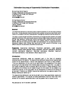
considered here. We consider the percentage monthly change in the monthly series in order to observe the growth rate. The graphical analysis of the rice inflation indicates the possible existence of unit root or structural break in the data that has to be checked. Figure (6): Structural Breaks in Basmati Rice Prices (January 2006-Fabruary 2011)

The model is: ( ) ( )

(

)

( ) (5.1)

The model being estimated passes all the diagnostic tests. Figure (7) gives the plot of the actual and the fitted monthly wheat inflation rate.

Figure (7): Actual and Fitted Basmati Rice Inflation rate (January 2006-Fabruary 2011)

Figures (8a, b, c, d) show the forecast and the actual inflation from the automatic regression estimated model over four different forecasting horizons and table (6) lists the 12 step forecasts using the model identified in equation 5.1. Pak.j.stat.oper.res. Vol.VIII No.1 2012 pp1-20

13


Figure (8):Forecast and the Actual Basmati Rice Inflation Rate ( ) from the Automatic Regression model for Four Forecasting Horizons

(a) h=1

(b) h=3

(c) h=6

(d) h=12

Table (6): 12-step forecast for Rice inflation Horizon Forecast SE 2010-9 -25.5466 9.28 2010-10 -24.5609 12.87 2010-11 -23.6132 15.47 2010-12 -22.702 17.53 2011-1 -21.826 19.24 2011-2 -20.9839 20.69 2011-3 -20.1742 21.95 2011-4 -19.3957 23.06 2011-5 -18.6473 24.03 2011-6 -17.9278 24.9 2011-7 -17.236 25.67 2011-8 -16.571 26.37 2011-9 -12.0455 26.37 2011-10 -2.82162 26.37 2011-11 -2.91578 26.37 2011-12 -1.29013 26.37 2012-1 3.75457 26.37 2012-2 4.48263 26.37 mean(Error) = 20.31 SD(Error) = 7.2901

( ) Actual -19.3152 -4.52453 -4.67552 -2.06875 6.02052 7.18799 .NaN .NaN .NaN .NaN .NaN .NaN .NaN .NaN .NaN .NaN .NaN .NaN RMSE MAPE

14


Error 6.23143 20.0363 18.9376 20.6333 27.8466 28.1718 .NaN .NaN .NaN .NaN .NaN .NaN .NaN .NaN .NaN .NaN .NaN .NaN = =

t-value 0.672 1.556 1.224 1.177 1.447 1.361 .NaN .NaN .NaN .NaN .NaN .NaN .NaN .NaN .NaN .NaN .NaN .NaN 21.578 455.33


The use of ARIMA model for forecasting purpose without attempting to detect the timing, size and nature of the structural change that has been occurred in the inflation procedure during the time period examined is not appropriate.

The resultant model through automatic model selection after capturing large outliers is: ( )

( )

(

( )

( ))

(

( )

( )) (

)

(

)

(

)

(

) (5.2)

The above model passes all diagnostic and normality tests namely the AR test (1-3 lags), the ARCH (1-3 lags) test, the Normality test, and the Hetero test. Figure (9) shows the graph of the actual and the fitted time series.

Figure (9): Actual and Fitted Time Series, Automatic Model Capturing Outliers.

Now using the above selected model for forecasting Figures (10a, b, c, d) show the forecast and the actual inflation from the impulse saturated regression over four different forecasting horizons.


15


Figure (10): Forecast and Actual Inflation using Impulse Regression over Four Forecasting Horizons

(a) h=1

(b) h=3

(c) h=6

(d) h=12

The following table (Table 7) shows the within sample forecasts with horizon 12.

Table (7): 12-step forecast for Rice inflation using Impulse Saturation Model Horizon 2010-9 2010-10 2010-11 2010-12 2011-1 2011-2 2011-3 2011-4 2011-5 2011-6 2011-7 2011-8 2011-9 16

Forecast -25.1512 -23.8064 -22.5336 -21.3288 -20.1884 -19.109 -18.0873 -17.1202 -16.2048 -15.3384 -14.5183 -13.7421 -9.98913

SE 6.771 9.323 11.12 12.52 13.65 14.58 15.38 16.05 16.63 17.14 17.58 17.96 17.96

Actual -19.3152 -4.52453 -4.67552 -2.06875 6.02052 7.18799 .NaN .NaN .NaN .NaN .NaN .NaN .NaN

Error 5.83601 19.2819 17.8581 19.26 26.2089 26.297 .NaN .NaN .NaN .NaN .NaN .NaN .NaN

t-value 0.862 2.068 1.606 1.539 1.921 1.803 .NaN .NaN .NaN .NaN .NaN .NaN .NaN



Horizon 2011-10 2011-11 2011-12 2012-1 2012-2 mean(Error) SD(Error)

6.

Forecast -2.33993 -2.41802 -1.06989 3.113605 3.717378 = =

SE 17.96 17.96 17.96 17.96 17.96 19.124 6.8296

Actual .NaN .NaN .NaN .NaN .NaN RMSE MAPE

Error .NaN .NaN .NaN .NaN .NaN = =

t-value .NaN .NaN .NaN .NaN .NaN 20.307 428.42

Conclusion:

In this paper we have attempted to improve the forecast from a univariate time series model by applying automatic regression model selection technique and impulse saturated modeling to identify the structural breaks. Using the impulse saturation technique helps in the identification of the exogenous breaks with economic events and in the development of certain leading inflation indicators. The wheat inflation series were considered, Using regression modeling without identifying the breaks leads to a model with RMSE equals to 7.7268 and MAPE equals to 472.15 as compared to the situation when identifying outliers with large residuals using G2S technique for model selection, the resulting model has RMSE equals to 1.0941 and MAPE equals to 65.505. This can also be observed by comparing the forecast errors for individual forecasts in table (3) and table (5). Similar results hold for the case of rice price data. When the model without incorporating the structural changes is identified using the ARIMA model listed in equation (5.1) having RMSE as 21.578and MAPE as 455.33. While considering the observations with large residuals, the model hence identified contains two exogenous breaks; first one in form of a regime shift over the period of April-2008 to April-2009 and another continuous but short term break at April 2009which has its effect up till May 2009. It is observed that this model is better for forecasting as it yields RMSE equals to 20.307 and MAPE of 428.42. We can conclude that the model performs poor without adjusting for the possible structural breaks in the series. Hence, the forecasts obtained after identifying the breaks using automatic model selection (Gets) with breaks provide better forecast than ignoring these breaks. References 1. Bai, J. and Perron, P. (1998). Estimating and testing linear models with multiple structural changes, Econometrica, 66, 47-78. 2. Bai, J. and Perron, P. (2003). Computation and analysis of multiple structural change models, Journal of Applied Econometrics, 18, 1-22. 3. Bond, D. and Harrison M. J. 1992. ‗Some recent developments in econometric model selection and estimation‘. The Statistician 41: 315-325.


17


4. Castle, Jennifer L., Fawcett, Nicholas W.P. and Hendry, David F. (2008). Forecasting with equilibrium-correction models during structural breaks, Discussion paper, Oxford University, No 408. 5. Clements, M. P., and D. F. Hendry (2008). Economic Forecasting in a Changing World. Capitalism and Society, Vol. 3, Issue 2. Article 1. 6. Clements, M. P., and D. F. Hendry (eds.) (2002). A Companion to Economic Forecasting, Blackwell Publishers, Oxford. 7. Clements, M. P., and Hendry, D. F. (1998). Forecasting Economic Time Series. Cambridge: Cambridge University Press. 8. Clements, M.P and Hendry, D.F. (1999). Forecasting Non-stationary Economic Time Series. Cambridge, MA: MIT Press, 1999. ISBN 0-26203272-4. xxviii + 262 pp. 9. Darnell, A. C. and Evans, J. L. 1990. The Limits of Econometrics. Aldershot: Edward Elgar Publishing. 10. David F. Hendry Unpredictability and the Foundations of Economic Forecasting, 2004-W15 in Nuffield Economics Research. 11. Engle, R. F., and Smith, A. D. (1998). Stochastic permanent breaks. Review of Economics and Statistics, 81, 553–574. 12. Engle, R. F., Hendry, D. F. and Richard, J. F. (1983). Exogeneity, Econometrica, 51, 277-304. 13. Engle, R.F. and D.F. Hendry (1993). Testing super exogeneity and invariance in regression models. Journal of Econometrics, 56, 119-139. 14. Ericsson, N.R. (2008). Comment on "Economic Forecasting in a Changing World" (by Michael Clements and David Hendry). Capitalism and Society: Discussion and Commentaries. Vol. 3, issue 2. 15. Federal Bureau of Statistics (FBS), http://www.statpak.gov.pk/fbs/ 16. Fildes, R., Makridakis, S., 1995. The impact of empirical accuracy studies on time series analysis and forecasting. International Statistical Review 63, 289-308. 17. Gilbert, C. L. (1986). Professor Hendry‘s Econometric Methodology. Oxford Bulletin of Economics and Statistics, 48 (3), 283-307.

18



18. Haywood, J. and Randal, J. (2007). Modeling seasonality and multiple structural breaks. Did 9/11 affect visitor arrivals to NZ Research Report 07-1, School of Mathematics, Statistics and Computer Science, Victoria University of Wellington, NZ. www.stat.uiowa.edu/timeseries/abstracts/haywood-paper.pdf 19. Hendry, D. 1980. ‗Econometrics - Alchemy or Science‘. Economica, 47:11:387-406. 20. Hendry, D. F. (2000). On detectable and non-detectable structural change. Structural Change and Economic Dynamics, 11, 45–65. Reprinted in The Economics of Structural Change, Hagemann, H. Landesman, M. and Scazzieri (eds.), Edward Elgar, Cheltenham, 2002. 21. Hendry, D. F. and Santos, C. (2007). Automatic Tests For Super Exogeneity, Working Papers in Economics 11, Faculdade de Economia e Gestão, Universidade Católica Portuguesa. 22. Hendry, D. F., and Doornik, J. A. (1997). The implications for econometric modeling of forecast failure. Scottish Journal of Political Economy, 44, 437–461. Special Issue. 23. Hendry, D. F., Johansen, S. and Santos, C. (2007). Selecting a Regression Saturated by Indicators, Discussion Papers 07-26, University of Copenhagen. Department of Economics (formerly Institute of Economics), revised. 24. Hendry, D.F., and Krolzig, H.-M. (2001). Automatic Econometric Model Selection. London: Timberlake Consultants Press. 25. James H. Stock & Mark W. Watson (1996). Asymptotically Median Unbiased Estimation of Coefficient Variance in a Time Varying Parameter Model. NBER Technical Working Papers 0201, National Bureau of Economic Research, Inc. 26. Leamer, E. E. 1983. ‗Lets take the con out of econometrics‘. American Economic Review 73:31-43. 27. Nielsen, B. and Johansen, S. (2007). Saturation by Indicators in Autoregressive Models, University of Oxford, Department of Economics, mimeo. 28. Pesaran, M. H. and Timmermann, A. (2004). How costly is it to ignore breaks when forecasting the direction of a time series? International Journal of Forecasting, 20, 411-425. Pak.j.stat.oper.res. Vol.VIII No.1 2012 pp1-20

19


29. Santos, C. (2007). A pitfall in joint stationarity, weak exogeneity and autoregressive distributed lag models, Economics Bulletin, vol. 3(53), pages 1-5. 30. Santos, C. (2008). Impulse saturation break tests, Economics Letters, vol. 98(2), pages 136-143. 31. Santos, C. and Hendry, D. F. (2006). Saturation in Autoregressive Models, Not as Económicas, issue 24, pages 8-19. 32. Stock, J. H., and Watson, M. W. (1999). A comparison of linear and nonlinear models for forecasting macroeconomic time series. In Engle, R. F., and White, H. (eds.), Cointegration, Causality and Forecasting, pp. 1– 44. Oxford: Oxford University Press. 33. West, M. and Harrison, P.J. (1998), Bayesian Forecasting and Dynamic Models, Springer Verlag.

20


Sampling Algorithm of Order Statistics for Conditional ...

Sampling Algorithm of Order Statistics for Conditional ...

Suggest Documents